EE178/278A: Probabilistic Systems Analysis, Spring 2014 (Tse)
Homework 9
Due Tues, June 3, 4pm
1. Practice with Markov chains
Consider the two-state Markov chain X1 , X2 , . . . , with Xi ∈ {0, 1} and symmetric transition probabilities
P (1|0) = P (0|1) = α and P (0|0) = P (1|1) = 1 − α (α < 0.5). Suppose the initial distribution
(distribution of X1 ) is π(0) = π(1) = 0.5.
a) Draw the state transition diagram.
Answer:
1−α
0
α
1
1−α
α
b) Compute the distribution of X2 .
Answer:
P(X2 = 0) = P(X2 = 0|X1 = 0)P(X1 = 0) + P(X2 = 0|X1 = 1)P(X1 = 1)
= (1 − α)P(X1 = 0) + αP(X1 = 1)
= (1 − α) × 0.5 + α × 0.5
= 0.5,
and P(X2 = 1) = 0.5 as well.
c) What is the distribution of Xn for general n?
Answer: Since the transition probabilities do not depend on time, we can repeat the argument with
X2 replacing X1 and X3 replacing X2 and obtain P(X3 = 0) = P(X3 = 1) = 0.5. Repeating this
argument, we see that P(Xn = 1) = P(Xn = 0) = 0.5 for all n.
d) Compute the joint distribution of X1 and X3 . Are these two random variables independent?
Answer: By total probability rule,
P(X1 = 1, X3 = 0) = P(X1 = 1, X3 = 0, X2 = 0) + P(X1 = 1, X3 = 0, X2 = 1)
1
= (P(X3 = 0, X2 = 0|X1 = 1) + P(X3 = 0, X2 = 1|X1 = 1))
2
1
= ((1 − α)α + (1 − α)α)
2
= α(1 − α).
Similarly, P(X1 = 0, X3 = 1) = α(1 − α).
1
(P(X3 = 0, X2 = 0|X1 = 0) + P(X3 = 0, X2 = 1|X1 = 0))
2
1
=
(1 − α)2 + α2
2
P(X1 = 0, X3 = 0) =
and P(X1 = 0, X3 = 0) = P(X1 = 1, X3 = 1).
Using part (c) we know that
P(X1 = 1)P(X3 = 0) =
1 1
1
× = 6= α(1 − α)
2 2
4
since α < 0.5. Therefore the two random variables are not independent.
e) Now suppose we have another sequence of random variables Y1 , Y2 , . . . with Yi ∈ {0, 1} and the Yi ’s
are mutually independent conditional on the Xi ’s. Further, suppose each Xi is connected to Yi through
a binary symmetric channel with crossover probability p < 0.5. Compute P(Y3 = 0|Y2 = 0) and
P(Y3 = 0|Y1 = 0, Y2 = 0). Do the Yi ’s form a Markov chain? Give an intuitive explanation of your
answer.
Answer: First, using the total probability rule, we compute P(Y2 = 0) and P(Y2 = 0, Y3 = 0) to be
P(Y2 = 0) = P(Y2 = 0, X2 = 0) + P(Y2 = 0, X2 = 1)
1
= (P(Y2 = 0|X2 = 0) + P(Y2 = 0|X2 = 1))
2
1
= ((1 − p) + p)
2
1
=
2
P(Y2 = 0, Y3 = 0) = P(Y2 = 0, Y3 = 0, X2 = 0, X3 = 0) + P(Y2 = 0, Y3 = 0, X2 = 0, X3 = 1)
+ P(Y2 = 0, Y3 = 0, X2 = 1, X3 = 0) + P(Y2 = 0, Y3 = 0, X2 = 1, X3 = 1)
1
= (P(X3 = 0|X2 = 0)P(Y2 = 0|X2 = 0)P(Y3 = 0|X3 = 0)
2
+ P(X3 = 1|X2 = 0)P(Y2 = 0|X2 = 0)P(Y3 = 0|X3 = 1)
+ P(X3 = 0|X2 = 1)P(Y2 = 0|X2 = 1)P(Y3 = 0|X3 = 0)
+ P(X3 = 1|X2 = 1)P(Y2 = 0|X2 = 1)P(Y3 = 0|X3 = 1))
1
=
(1 − α)(1 − p)2 + 2α(1 − p)p + (1 − α)p2
2
Therefore,
P(Y3 = 0|Y2 = 0) = (1 − α)(1 − p)2 + 2α(1 − p)p + (1 − α)p2 .
Now P(Y1 = 0, Y2 = 0) = P(Y2 = 0, Y3 = 0). Let A be the event that {Y1 = 0, Y2 = 0, Y3 = 0}.
We write P(A) as
X
P(A) =
P(A, X1 = i, X2 = j, X3 = k)
i,j,k∈{0,1}
=
1
2
X
P(Y1 = 0|X1 = i)P(Y2 = 0|X2 = j)P(Y3 = 0|X3 = k)
i,j,k∈{0,1}
· P(X1 = i)P(X2 = j|X1 = i)P(X3 = k|X2 = j)
1
= (1 − α)2 p3 + (1 − α)2 (1 − p)3 + 2α(1 − α)p2 (1 − p) + 2α(1 − α)(1 − p)2 p
2
+ α2 (1 − p)2 p + α2 p2 (1 − p).
Finally we get that
P(Y3 = 0|Y2 = 0, Y1 = 0) =
1
2
((1 − α)(1 −
p)2
P(A)
.
+ 2α(1 − p)p + (1 − α)p2 )
We see that the two probabilities P(Y3 = 0|Y1 = 0, Y2 = 0) and P(Y3 = 0|Y2 = 0) are not equal.
Therefore the Yi s do not form a Markov chain. Intuitively, Yi does not contain all the necessary past
information because it is not exactly equal to Xi . Hence, having further information from Yi−2 , Yi−3
etc. provides more information about Xi .
2. Continuous observations
In class when we discussed the communication and speech recognition problems, we assumed the observed
outputs Yi ’s are discrete random variables. For physical channels, this is an appropriate model if the Yi ’s
are discretizations of the underlying continuous signals. Often though, one may want to model directly
the continuous received signals, in which case it is natural to treat the Yi ’s as continuous random variables.
Everything we did goes through, except that we need to replace the conditional probability of the observation
given the input by the conditional pdf of the observation given the input. (You can assume this fact for the rest
of the question, but you may want to think a bit why this is valid, by thinking of the continuous observation
as a limit of discretization as the discretization interval δ goes to zero.)
a) In the repetition coding communication example, suppose Yi ∼ N (A, σ 2 ) when X = 0 is transmitted,
and Yi ∼ N (−A, σ 2 ) when X = 1 is transmitted. (Physically, we are sending a signal at voltage level
A to represent a 0 and at voltage level −A to represent a 1, and there is an additive noise corrupting
the transmitted signal to yield the received signal.). Re-derive the MAP receiver (decision rule) for this
channel model. Put it in the simplest form.
Answer: The MAP receiver rule derived in Lecture 15 was:
LLR(b1 , · · · , bn ) :=
n
X
LLR(bi )
i=1
X̂=0
≷
X̂=1
log
1−α
α
.
The difference when Yi is continuous is that
1
f (Y = b|X = 0)
= 2 (b + A)2 − (b − A)2 .
LLR(b) = log(L(b)) = log
f (Y = b|X = 1)
2σ
Therefore the overall rule is
n
1 X
(bi + A)2 − (bi − A)2
2σ 2
i=1
X̂=0
≷
X̂=1
log
1−α
α
.
b) In the speech recognition example, suppose Yi ∼ N (µa , σ 2 ), when Xi = a. (µa ’s and σ 2 are then
parameters of the model which are assumed to be known.) Compute the edge costs d(a) and di (a, a0 )
of the Viterbi algorithm for this channel model. Be as explicit as you can.
Answer: From the definitions in Lecture 17,
d(a) = − log(π(a)Q(b|a))
−(b1 −µa )2
1
2
= − log(π(a)) − log √
e 2σ
2πσ 2
√
(b1 − µa )2
2 .
= − log(π(a)) −
+
log
2πσ
2σ 2
and
di (ai , ai−1 ) = − log(p(ai |ai−1 )) −
√
(bi − µai )2
2 .
+
log
2πσ
2σ 2
This edge cost is the sum of three terms. The first term depends on the likelihood of transitioning from
state ai−1 to state ai . The second term depends to how close the state ai for Xi fits the observation
Yi = bi . The third term is a constant and can be ignored.
© Copyright 2026 Paperzz