Mathematical Modeling with LPL Tony Hürlimann Department of Informatics , University of Fribourg Bd. Perolles 90 1700 Freiburg [email protected] You can download this lecture at : www.virtual-optima.com/download/docs/lpl-lecture.pdf Mathematical Optimization 1 Overview Simple Access to Mathematics Mathematics – Reality A game Slitherlink Route planning Color vertices – exams schedules ? „Real“ Examples : Work schedule für bus drivers Cutting of paper rolls Location and Logistics (Supply-Chain) Rostering: Work schedule of 800 persons at the Zurich aeroport ! Mathematical Optimization 2 A simple game Problem : Two players play the following number game: Each chooses (secretly) a positive number. The numbers are then uncovered at the same time and compared. If the numbers are equal, neither of the players will get a payoff. If the numbers differ by one, then the player who has chosen the higher number obtains the sum of both, otherwise the player with the smaller number obtains the smaller of both. The play is repeated endlessly. Which number and how often should a player choose a number in each round? 4 1 2 1 1 4 4 2 3 3 Table of Numbers from which you can choose (optimally) [ above we choose from the row 1 1 third 4 1 2 3 2 1 ]2: 2 1 3 1 4 1 2 5 2 4 2 3 4 4 2 1 2 3 1 4 2 3 1 5 2 4 5 3 5 4 1 1 1 3 1 3 1 4 3 4 4 3 4 1 2 1 3 1 1 5 3 4 4 3 2 4 1 2 3 3 1 3 1 2 1 5 1 5 3 3 5 3 4 2 5 3 1 5 4 3 3 5 3 1 2 4 3 1 1 3 3 3 3 1 2 2 3 3 1 1 3 1 4 1 4 5 1 4 3 1 1 2 4 3 2 5 1 5 3 5 4 2 5 4 2 3 4 1 4 5 1 3 1 5 3 2 5 5 1 2 5 2 1 3 1 1 1 4 1 2 1 1 1 1 1 1 1 5 1 1 1 4 3 3 1 1 4 5 1 3 2 3 5 4 3 1 2 2 1 4 2 3 2 1 1 1 2 1 1 1 4 1 4 2 3 4 5 5 2 5 3 2 3 4 2 3 3 2 1 3 3 2 3 3 3 5 3 3 4 2 4 3 5 5 3 1 5 2 2 2 2 2 3 1 3 2 2 1 3 3 2 3 3 4 5 2 4 1 5 2 4 5 4 4 3 4 4 1 3 4 2 3 5 2 4 1 3 3 5 3 2 5 3 5 4 5 3 3 5 1 4 1 3 1 2 2 1 1 5 5 2 5 2 2 3 2 3 3 2 1 1 1 4 1 1 3 3 4 3 1 4 3 2 3 1 1 2 2 1 1 3 2 4 1 1 3 4 2 5 3 3 5 4 1 1 4 3 3 5 1 5 How was this table built and why should this be „optimal“? (see next page!) Mathematical Optimization 3 The game: math. Formulation Mathematical Formulation Numbers to choose : i, j 1...n Pay matrix : pi , j if i j 1, i j if i j 1 j 0 if i j i j if i j 1, j if i j 1 The optimal strategy of a player is: Unknown : the frequences xi Condition : n i 1 xi 1 Choose number 1 with frequency 24.75% Choose number 2 with frequency 18.81% Choose number 3 with frequency 26.73% Choose number 4 with frequency 15.84% Choose number 5 with frequency 13.86% Never choose another number ! (Both players can follow this strategy, then in the long run nobody will win!) n M inimize the loss : min max i 1 pi , j xi j1...n Computer-excutable Form model GAME; set i, j := /1:100/; parameter p{i,j} := if(i>j+1,-j , i=j+1,i+j , i=j-1,-i-j, i<j-1,i); variable x{i} "Strategy"; constraint R: sum{i} x = 1; maximize gain: min{j}(sum{i} p*x); end The table on the previous page was built on these frequencies ! Coded in the mathematical Modeling Language LPL SEE: http://lpl.unifr.ch/lpl/Solver.jsp?name=gameh Mathematical Optimization 4 Sudoku model sudoku; parameter S; set i, j,k : 1..S^2; set h, g: 1..S; parameter P{i,j}; // Read from file: S, P binary variable x{i,j,k}; constraint N{i,j}: sum{k} x = 1; R{i,k}: sum{j} x = 1; C{j,k}: sum{i} x = 1; B{h,g,k}: sum{h1=h,g1=g} x[(h-1)*S+h1,(g-1)*S+g1,k] = 1; F{i,j,k|P[i,j]=k}: x = 1; maximize any: x[1]; end A model with:15’625 variables and 2’787 linear constraints This is a complete specification. SEE: http://lpl.unifr.ch/lpl/Solver.jsp?name=sudoku Mathematical Optimization 5 Slitherlink : Another game like Sudoku Find a round-trip that follows the borders of the cells and contains as many line segment as the number says : A Slitherlink Puzzle .... and its solution 6 Mathematical Optimization Slitherlink: Solution Try to solve it: Special configuration: 1 at a corner, 3 und 0! The 2 in a bottom line The 3 in a corner etc. Solution using a mathematical model! In the Internet you can run various puzzles: SEE: http://lpl.unifr.ch/lpl/Solver.jsp?name=slitherlink 7 Mathematical Optimization Mathematics is everywhere Manufacture cans: Minimal usage of material ! How should be the relation between height and width of a can ? Volume h r 1 ( Liter ) 2 h=height , r=radius Surface 2 r 2 2 r h minimize S 2 r2 Surface 2 r With a radius of 0.8dm the height will be only 0.5dm and the surface then is 6.5dm2, hence 18% heigher than in ist minimum ! O 5.54dm2 h r 3 1 2 0.542dm, h 3 4 2 r 2.02 1.09dm r=radius SEE: http://lpl.unifr.ch/lpl/Solver.jsp?name=can Mathematical Optimization 8 Mathematics is everywhere Ciphering while transfering electronic money : To multiple two large number is simple ! To factor a large number into its (two) prime numbers is difficult ! Everybody can (with a little patience) do the folowing multiplication : 193'707'721 * 761'838'257'287 = 147'573'952'589'676'412'927 ! But: The mathematicien Cole (1861–1926) spent his weekends of 3 years to factor the number 267-1 = 147'573'952'589'676'412'927 into its two prim factors:193'707'721 und 761'838'257'287. This assymetry in the complexity is used in real-life cryptography, to cipher a text in a simple way. However, the text cannot be easily deciphered ! If you know the two prime factors, you can decipher a text ! If you know only the result of the multiplication, you can encipher ! Mathematical Optimization 9 Learning LPL: Some Links A Short Introduction www.virtual-optima.com/download/docs/puzzbook-chap1.pdf Other Papers www.virtual-optima.com/en/papers.html Download LPL www.virtual-optima.com/de/download.html Learning Through Many Models lpl.unifr.ch/lpl/mainmodel.html Mathematical Optimization 10 Route Planning (I) A larger distributor in the region of Berne : Has 12 trucks of 3½ tons. Delivers electrical material to ~600-700 clients each day (night). The trucks must not be overloaded. The tour must not be longer than 6 hours. The total of distance traveled should be as small as possible (save cost and time). 11 Mathematical Optimization Route Planning (II) Tour l km 284 Locations 21 Clients 39 Time 7.63 Costs 1061.67 ------------------Tour L km 182 Locations 21 Clients 39 Time 5.60 Costs 807.79 Distance of a „really“ traveled tour (March 2006) „Optimally“ traveled tour (shortest tour) Savings: Time : 2 hours Costs: FR 264.-12 Mathematical Optimization Route Planning (III) Tour 2 (black) km 275 Locations 34 Clients 59 Time 8.45 Costs 1219.64 -----Tour 3 (blue) km 192 Locations 22 Clients 43 Time 6.00 Costs 868.34 -----Total 2087.99 FR 467 km Better tours 2 and 3 see next pages ! „Really“ traveled tours 2 and 3 (March 2006) 13 Mathematical Optimization Route Planning (III) Tour 2 (black) km 197 Locations 30 Clients 49 Time 6.39 Costs 934.05 -----Tour 3 (blue) km 204 Locations 25 Clients 53 Time 6.74 Costs 988.8 -----Total 1922.85 FR 401 km Optimal unbundling of tour 2 and 3 Savings: Time : 1.5 hours Costs: FR 165.— Benefit : 66 km 14 Mathematical Optimization Route Planning (IV) Tour 1 km 302 Locations 34 Clients 118 Time 11.95 Costs 1818.57 -----Tour 2 km 324 Locations 51 Clients 120 Time 12.48 Costs 1890.30 -----Tour e km 0 Locations 0 Clients 0 Time 0 Costs 0 -----Total 3708.87 FR 20.30h00. Starting Time Last client at 9.30h00 -- it is too late! Mathematical Optimization Too much Two „overloaded“ tours : Spit into an additional tour „e“ See next page. 15 Route Planning (IV) Tour 2 Tour 1 Tour e Starting Time 20.30h00. All clients served before 5.30h00 ! Tour 1 km 212 Locations 17 Clients 82 Time 8.34 Costs 1269.24 -----Tour 2 km 236 Locations 34 Clients 81 Time 8.78 Costs 1320.56 -----Tour e km 252 Locations 34 Clients 75 Time 8.80 Costs 1306.75 -----Total 3896.56 FR Now balanced Additional costs only at: 187.70 FR 16 Mathematical Optimization Route Planning (V) : A Demo Collect children in a village with two buses http://lpl.unifr.ch/lpl/Solver.jsp?name=/schoolbus A small paper (in German) www.virtual-optima.com/download/docs/astagOK-de.pdf 17 Mathematical Optimization Mathematics: How does it work ? „Abstract“ Problem: Vertex coloring Graph consists of vertices and edges Example: net with locations and routes A abstract problem (just baublery !?) Is this useful ? Well .... 4 colors are necessary at least. How many colors do we need for the vertices such that two neighbors do not have the same color ? 18 Mathematical Optimization Mathematics: How does it work ? Exams schedule A number of exams, a number of students How to find a Conflict-free schedule! Correspondence Mathematics – „Reality“ : Vertex = Edge = Color = Number of colors = Time Time Time Time Window Window Window Window 1 2 3 4 Exam Collision Time window Length of schedule : : : : Exams Exams Exams Exams No.: No.: No.: No.: 1 3 2 5 6 4 8 9 7 10 19 Mathematical Optimization Mathematikcs: How does it work ? Semaphores at a crossroads Number of traffic lanes, Number of cossing roads Collision-free plan of phases ? Correspondence Mathematics – „Reality“ : Vertex = Edge = Color = Number of colors = Time Time Time Time window window window window 1 2 3 4 : : : : Traffic Lane Collision Time Window Length of phases Exams Exams Exams Exams No.: No.: No.: No.: 1 4 9 11 12 13 3 6 8 5 7 10 2 20 Mathematical Optimization Alternative solution Semaphores at a crossroads Number of traffic lanes, Number of cossing roads Collision-free plan of phases ? Correspondence Mathematics – „Reality“ : Vertex = Edge = Color = Number of colors= Time Time Time Time window window window window 1 2 3 4 Traffic Lane Collision Time window Length of phases : : : : Exams Exams Exams Exams No.: No.: No.: No.: 1 2 3 4 5 6 13 10 11 12 7 8 9 21 Mathematical Optimization Larger Problems ! 100 Exams! 24 time windows More difficult to solve. Needs math. methods ! Needs computer power 22 Mathematical Optimization This is the mathematical model of the vertex coloring Let : I {1...n} with n 0 and : G I I We are looking for K minimal (with 0 K n ) such that : (1) x ik k{1K } 1 for all i I (2) xik x jk 1 for all k {1 K }, (i, j ) G We shall go through this model later in the course ! SEE: http://lpl.unifr.ch/lpl/Solver.jsp?name=coloring2 http://lpl.unifr.ch/lpl/Solver.jsp?name=coloring1 23 Mathematical Optimization Schedule: How many bus drivers ? Number of excursions planed Problem: How many drivers need to be hired? Monday: 14, Tuesday: 12, Wendesday: 18, Thursday: 16, Friday: 15, Saterday: 16, Sunday: 19 At least 19 (see Sunday)! Well! It depends on the working plan maximally 5-days working 2 consecutive free days 24 Mathematical Optimization Schedule: Formulation 7 working contracts (5 days consecutive) -----------------------------------------------------Mo Tu We Th Fr Sa Su D1 * * * * * D2 * * * * * D3 * * * * * D4 * * * * * D5 * * * * * D6 * * * * * D7 * * * * * Unknown quantities (Number of drivers under the 7 different working contracts) -----------------------------------------------------D1 D2 D3 D4 D5 D6 D7 x1 x2 x3 x4 x5 x6 x7 Operation schedule (Number of drivers per day) -----------------------------------------------------Mo : x1 + x4 + x5 + x6 + x7 ≥ 14 Di : x1 + x2 + x5 + x6 + x7 ≥ 12 . . . Mathematical Model MODEL Plans "Schedule of Drivers"; INTEGER VARIABLE x1; x2; x3; x4; CONSTRAINT mon: + x1 + x4 + x5 + x6 + x7 die: + x1 + x2 + x5 + x6 + x7 mit: + x1 + x2 + x3 + x6 + x7 don: + x1 + x2 + x3 + x4 + x7 fre: + x1 + x2 + x3 + x4 + x5 sam: + x2 + x3 + x4 + x5 + x6 son: + x3 + x4 + x5 + x6 + x7 MINIMIZE obj: + x1 + x2 + x3 + x4 + x5 END x5; x6; x7; >= >= >= >= >= >= >= 14; 12; 18; 16; 15; 16; 19; + x6 + x7; Solution on a computer SEE: http://lpl.unifr.ch/lpl/Solver.jsp?name=plaene 25 Mathematical Optimization Schedule: Various Solutions 5 Plans with 2 to 6 different working contracts : 2 contracts 1 2 Mo 14 Tu 14 We Th Fr Sa Su 19 19 19 19 19 33 drivers , 123 total salary DEMAND 14 12 18 16 15 16 19 Actual 14 14 19 19 19 19 19 Overplus 0 2 1 3 4 3 0 -----------------------------------------3 contracts Mo Di Mi Do Fr Sa So 1 3 3 3 3 2 11 11 3 16 16 16 16 16 30 drivers , 114 total salary DEMAND 14 12 18 16 15 16 19 Actual 14 14 19 16 16 16 19 Overplus 0 2 1 0 1 0 0 -----------------------------------------4 contracts Mo Di Mi Do Fr Sa So 1 5 5 5 5 5 2 8 8 8 8 3 6 6 6 6 6 4 5 5 5 5 5 24 drivers , 112 total salary DEMAND 14 12 18 16 15 16 19 Actual 14 13 18 16 16 16 19 Overplus 0 1 0 0 1 0 0 5 contracts 1 2 3 4 5 Mo 3 2 9 Di 3 Mi 3 Do 3 7 Fr Sa 7 2 7 So 3 7 9 9 9 9 6 6 6 27 drivers , 110 total salary DEMAND 14 12 18 16 15 16 19 Actual 14 12 18 16 15 16 19 Overplus 0 0 0 0 0 0 0 -----------------------------------------6 contracts Mo Di Mi Do Fr Sa So 1 4 4 4 4 4 2 8 8 8 8 8 3 2 2 2 2 2 4 2 2 2 2 2 5 3 3 3 3 3 6 3 3 3 3 3 22 drivers , 110 total salary DEMAND 14 12 18 16 15 16 19 Actual 14 12 18 16 15 16 19 Overplus 0 0 0 0 0 0 0 26 Mathematical Optimization Problem: Cutting material Given paper rolls must be cut into demanded sizes such that the waste is minimized. 27 Mathematical Optimization Cutting: An example Widths of the rolls: 152cm , 122cm , 102cm. Demanded sizes (rectangles) : 20000 pieces of 24x 33 cm , 15000 pieces of 36x 80 cm , 5000 pieces of 29x100 cm 5000 pieces of 39x103 cm , 5000 pieces of 29x100 cm , 5000 pieces of 39x 93 cm 5000 pieces of 19x 75 cm , 15000 pieces of 29x 68 cm , 15000 pieces of 19x 29 cm Conditions: • 2-stage Guiottinen-cuts • First generate larger rectangles of length between 50 and 170cm (how?) • Rotatation of rectangles of 90º is ok. Problem: How many and in what length should the larger rectangles be cut into and how should the final rectangles then be cut from them in order to minimize the waste ? 28 Mathematical Optimization Cutting: Draft of solution 1) 2) Generate all optimal 2-stage unconstraint two-dimensional solutions: (How to cut optimally from width (102,122,152) and Length = [50..170] the smaller rectangles. Use these generated patterns in the following mathematical MIP-model : model stripcut "Cutting Rolls into Sheets"; set n "The different rectangles"; p "The patterns"; parameter B{n} "Number of rectangles to be cut"; w{n} “Width of the rectangles"; h{n} "Height of the rectangles"; a{p,n} "The number of rectangles in a pattern"; READ '%1:Table' FROM '2D-2X9.INP.txt'; --…read the data… integer variable x{p} [0,20000]; PP{n} "Positive deviation from the demanded number"; NN{n} "Negative deviation from the demanded number"; minimize obj: sum{n} 100000*(NN+PP) + sum{p} waste*x constraint AA{n}: SUM{p} a*x - PP + NN = B; end 29 Mathematical Optimization Cutting: Solution total usage of raw material total area of the rectangles total waste total waste (cross-check) percentage waste check whether the demand 1 , 24.0 x 33.0 , 2 , 36.0 x 80.0 , 3 , 29.0 x 100.0 , 4 , 39.0 x 103.0 , 5 , 29.0 x 100.0 , 6 , 39.0 x 93.0 , 7 , 19.0 x 75.0 , 8 , 29.0 x 68.0 , 9 , 19.0 x 29.0 , in in in in cm^2 cm^2 cm^2 cm^2 = = = = = is satisfied 20000 , 20000 15000 , 15000 10000 , 10000 5000 , 5000 0 , 0 5000 , 5000 5000 , 5000 15000 , 15000 15000 , 15000 display the sheets in detail roll-width sheet-height waste 152 100 169 152 106 144 152 150 0 152 156 214 152 165 255 152 168 72 122 68 245 122 78 57 122 117 19 122 156 29 102 103 96 102 145 178 102 160 247 sheet structure 152-100 [3,3,3,3,(18,2)] 122-117 [(9,9,9,9),(13,13,13)] 122-68 [8,8,8,(18,10,10)] ……………… nr-sheets 1755 1 207 1 332 1 1 1356 762 1249 1 2498 2979 172920474.00 171230000.00 1690474.00 1690474.00 0.99% Examples from the solution : 1755 pieces : 152cm x 100 TOTWASTE 296595 144 0 214 84660 72 245 77292 14478 36221 96 444644 735813 762 pieces : 122cm x 117 1 pieces : 122cm x 68 ... Further pattern... 30 Mathematical Optimization Location and Transport Logistics Company Holcim uses LPL in its strategic and operative logistics. Problem: Decide where to produce, to pack ciment and in what quantities and how to transport to the clients in order to minimize costs. The mathematical structure (the business logic) consists can be written down on two A4-pages. The data are read/write to/from databases. The whole model consists of more than 10‘000 variables and constraints and can be solved in a few seconds on a current personal computer. 31 Mathematical Optimization Location and Transport Logistics (Holcim) Mathematical Optimization 32 Rostering at the aeroport of Zurich: Working plan Current project with FH Winterthur+Software company+client at the aeroport ZH 800 persons with different skills and contracts. 250 work shifts: Check-in (Swiss), announcement, ticket controls, etc. Monthy plan (30 days): Who works at which day in which shift ? Demand must be fulfilled Working laws and collective contracts must be observed and the skills must match. Maximize „Satisfaction“ 33 Mathematical Optimization Rostering at the aeroport of Zurich: Working plan Such problems can be treated and „solved“ with current techniques of Operations : 500‘000 variables 20‘000-40‘000 linear constraints To compare: look at this small trivial example with 2 variables and 2 linear constraints : „My grandfather and grandmother are together 150 years old. Theirs difference is 4 years. How old are both?“ (x = Age of grandfather, y = Age of grandmother) The model is { x + y = 150 x=y+4 The solution is { x = 77 x = 73 34 Mathematical Optimization Rostering at the aeroport : A Part of the mathematical model model Solution6 alias sol6; -- same as model sol5 but now backwards in i SetSolver(cplexLSolm,'BRDIR 1;TILIM 1000‘); Read('snap1.sps'); parameter diff:=10; lo:=#i-diff; constraint AssignPerson{Id[d,i]|~ii} : SUM{s|Isd[s,d,i]} x[s,d,i] = 1; CoverDemand{Sd[d,s]} : SUM{i|Isd[s,d,i] and ~ii} x[s,d,i] >= b[d,s]; TargetWorkload{i|~ii}: SUM{s,d|Isd[s,d,i]} (e[s]*x[s,d,i]) + dNeg[i]-dPos[i] = h[i]; while (lo-diff>0) (*and lo=0*) do minimize obj 'keep': sum{i|i>lo and i<=lo+diff} (dNeg+dPos); dummy:= {Isd[s,d,i]|i>lo and i<=lo+diff}(pX:=x); dummy:= {i|~ii} (pdPos:=dPos, pdNeg:=dNeg); addconst BND1{Isd[s,d,i]|i>lo and i<=lo+diff}: x=pX; addconst BND2{i|i>lo and i<=lo+diff}: dPos=pdPos; addconst BND3{i|i>lo and i<=lo+diff}: dNeg=pdNeg; lo:=lo-diff; end SaveSolution; This Code generates the end complete model with 500‘000 variables und 30‘000 constraints ! Mathematical Optimization 35 Rostering: Modules for an automatical solution process At the present time, 20 Persons are in charge to planify the schedules ! Decreasing importance for solving the problem! Efficient way to „translate“ the problem into the „right“ mathematical structure (Modelling). Mathematical toolboxes to solve the problem: Operations Research develops since 60 years powerful methods (Solution methods). Computer science: Inplement the approach together with user-interfaces and data binding (Programming). Needs fast computers (Hardware). 36 Mathematical Optimization Rostering: Extract of a solution Unsatisfying solution. Working time partially massively exceeded ! Persons Day in month Shift No 135 Distance between shifts too short Overtime (in 1/4 hours) 37 Mathematical Optimization Rostering: Extract of a solution This is a better solution. However, still violates working laws ! 38 Mathematical Optimization Rostering: Extract of the mathematical model MODEL DrawPlan,draw; Read('report1.sps'); parameter m "actual line"; n:=50 "page length"; K:=110 "total length (should be #i)"; co; red:=rgb(255,0,0); grey1:=rgb(230,230,230); grey2:=rgb(200,200,200); lBlue:=rgb(0,0,200); Draw.Scale(15,12); for{i,d|i<=K} do m:=(i-1)%n+1; --line co:=if((d-sunday)%7=0,grey2,(d-sunday+1)%7=0,grey1,1); if m=1 then -- page header Draw.Rect(d+2,0,d+3,1,co); Draw.Line(d+2,0,d+2,1,0,1); Draw.Text(d&' ',d+2.2,0,0,8,0); end if d=1 then Draw.Line(2,m,4,m); Draw.Line(2,m+1,4,m+1); Draw.Text(i&' ',0,m,0,8,0); end Draw.Rect(d+2,m,d+3.1,m+1.1,co,0,1); if idX then Draw.Text(idX&' ',d+2.1,m+.1,0,5,0); if idR<44 then Draw.Rect(PV+2+g[idX[PV,i]]/96,m+.6,d+2+f[idX]/96,m+1,red); end if idR<32 then Draw.Rect(PV+2+g[idX[PV,i]]/96,m+.6,d+2+f[idX]/96,m+1,0); end else if Id then Draw.Rect(d+2,m,d+3.1,m+1.1,lBlue,0,1); end Draw.Line(d+2,m,d+3,m+1); Draw.Line(d+2,m+1,d+3,m); end if d=#d then Draw.Text((PN)&' ',#d+4,m,0,8,0); Draw.Line(#d+6,m,#d+6,m+1); if m=n or i=K then Draw.Save(ceil(i/n)&'.svg'); end end This code generates the comend plete graph (previous page) end 39 Mathematical Optimization Summary Standardsoftware: just buy them Relatively well structured, repeated realms Text processing, accounting, etc. „Packages of various industries“ ... Time tabling in high school, and others. Machine control processes Complex decisions problems Schedules of all sorts Good Modeling skills are in high demand ! Layout-, LocationGood Solution methods needed ! rostering-, processes- Software: Rapid-Prototyping ! Hardware: the faster the better ! 40 Mathematical Optimization
© Copyright 2026 Paperzz