Observation of η_{c}(1S) and η_{c}(2S) decays to K^{+}K^{-}π^{+}
π^{-}π^{0} in two-photon interactions
The Harvard community has made this article openly available.
Please share how this access benefits you. Your story matters.
Citation
Del Amo Sanchez, P., J. P. Lees, V. Poireau, E. Prencipe, V.
Tisserand, J. Garra Tico, E. Grauges, et al. 2011. “Observation of
η_{c}(1S) and η_{c}(2S) Decays to K^{+}K^{-}π^{+}π^{}π^{0} in Two-Photon Interactions.” Physical Review D 84, no.
1: 012004.
Published Version
doi:10.1103/PhysRevD.84.012004
Accessed
June 15, 2017 4:13:40 AM EDT
Citable Link
http://nrs.harvard.edu/urn-3:HUL.InstRepos:13579262
Terms of Use
This article was downloaded from Harvard University's DASH
repository, and is made available under the terms and conditions
applicable to Open Access Policy Articles, as set forth at
http://nrs.harvard.edu/urn-3:HUL.InstRepos:dash.current.terms-ofuse#OAP
(Article begins on next page)
BABAR-PUB-10/022
SLAC-PUB-14406
hep-ex/1103.3971
arXiv:1103.3971v2 [hep-ex] 20 May 2011
Observation of ηc (1S) and ηc (2S) decays to K + K − π + π − π 0 in two-photon interactions
P. del Amo Sanchez,1 J. P. Lees,1 V. Poireau,1 E. Prencipe,1 V. Tisserand,1 J. Garra Tico,2 E. Grauges,2
M. Martinelliab ,3 A. Palanoab,3 M. Pappagalloab,3 G. Eigen,4 B. Stugu,4 L. Sun,4 M. Battaglia,5 D. N. Brown,5
B. Hooberman,5 L. T. Kerth,5 Yu. G. Kolomensky,5 G. Lynch,5 I. L. Osipenkov,5 T. Tanabe,5 C. M. Hawkes,6
A. T. Watson,6 H. Koch,7 T. Schroeder,7 D. J. Asgeirsson,8 C. Hearty,8 T. S. Mattison,8 J. A. McKenna,8
A. Khan,9 A. Randle-Conde,9 V. E. Blinov,10 A. R. Buzykaev,10 V. P. Druzhinin,10 V. B. Golubev,10
A. P. Onuchin,10 S. I. Serednyakov,10 Yu. I. Skovpen,10 E. P. Solodov,10 K. Yu. Todyshev,10 A. N. Yushkov,10
M. Bondioli,11 S. Curry,11 D. Kirkby,11 A. J. Lankford,11 M. Mandelkern,11 E. C. Martin,11 D. P. Stoker,11
H. Atmacan,12 J. W. Gary,12 F. Liu,12 O. Long,12 G. M. Vitug,12 C. Campagnari,13 T. M. Hong,13 D. Kovalskyi,13
J. D. Richman,13 C. West,13 A. M. Eisner,14 C. A. Heusch,14 J. Kroseberg,14 W. S. Lockman,14 A. J. Martinez,14
T. Schalk,14 B. A. Schumm,14 A. Seiden,14 L. O. Winstrom,14 C. H. Cheng,15 D. A. Doll,15 B. Echenard,15
D. G. Hitlin,15 P. Ongmongkolkul,15 F. C. Porter,15 A. Y. Rakitin,15 R. Andreassen,16 M. S. Dubrovin,16
G. Mancinelli,16 B. T. Meadows,16 M. D. Sokoloff,16 P. C. Bloom,17 W. T. Ford,17 A. Gaz,17 M. Nagel,17
U. Nauenberg,17 J. G. Smith,17 S. R. Wagner,17 R. Ayad,18, ∗ W. H. Toki,18 H. Jasper,19 T. M. Karbach,19
J. Merkel,19 A. Petzold,19 B. Spaan,19 K. Wacker,19 M. J. Kobel,20 K. R. Schubert,20 R. Schwierz,20
D. Bernard,21 M. Verderi,21 P. J. Clark,22 S. Playfer,22 J. E. Watson,22 M. Andreottiab ,23 D. Bettonia ,23
C. Bozzia ,23 R. Calabreseab,23 A. Cecchiab ,23 G. Cibinettoab ,23 E. Fioravantiab ,23 P. Franchiniab ,23 E. Luppiab ,23
M. Muneratoab ,23 M. Negriniab ,23 A. Petrellaab ,23 L. Piemontesea ,23 R. Baldini-Ferroli,24 A. Calcaterra,24
R. de Sangro,24 G. Finocchiaro,24 M. Nicolaci,24 S. Pacetti,24 P. Patteri,24 I. M. Peruzzi,24, † M. Piccolo,24
M. Rama,24 A. Zallo,24 R. Contriab ,25 E. Guidoab ,25 M. Lo Vetereab ,25 M. R. Mongeab ,25 S. Passaggioa,25
C. Patrignaniab,25 E. Robuttia ,25 S. Tosiab ,25 B. Bhuyan,26 V. Prasad,26 C. L. Lee,27 M. Morii,27 A. Adametz,28
J. Marks,28 U. Uwer,28 F. U. Bernlochner,29 M. Ebert,29 H. M. Lacker,29 T. Lueck,29 A. Volk,29 P. D. Dauncey,30
M. Tibbetts,30 P. K. Behera,31 U. Mallik,31 C. Chen,32 J. Cochran,32 H. B. Crawley,32 L. Dong,32
W. T. Meyer,32 S. Prell,32 E. I. Rosenberg,32 A. E. Rubin,32 A. V. Gritsan,33 Z. J. Guo,33 N. Arnaud,34
M. Davier,34 D. Derkach,34 J. Firmino da Costa,34 G. Grosdidier,34 F. Le Diberder,34 A. M. Lutz,34 B. Malaescu,34
A. Perez,34 P. Roudeau,34 M. H. Schune,34 J. Serrano,34 V. Sordini,34, ‡ A. Stocchi,34 L. Wang,34 G. Wormser,34
D. J. Lange,35 D. M. Wright,35 I. Bingham,36 C. A. Chavez,36 J. P. Coleman,36 J. R. Fry,36 E. Gabathuler,36
R. Gamet,36 D. E. Hutchcroft,36 D. J. Payne,36 C. Touramanis,36 A. J. Bevan,37 F. Di Lodovico,37 R. Sacco,37
M. Sigamani,37 G. Cowan,38 S. Paramesvaran,38 A. C. Wren,38 D. N. Brown,39 C. L. Davis,39 A. G. Denig,40
M. Fritsch,40 W. Gradl,40 A. Hafner,40 K. E. Alwyn,41 D. Bailey,41 R. J. Barlow,41 G. Jackson,41 G. D. Lafferty,41
J. Anderson,42 R. Cenci,42 A. Jawahery,42 D. A. Roberts,42 G. Simi,42 J. M. Tuggle,42 C. Dallapiccola,43
E. Salvati,43 R. Cowan,44 D. Dujmic,44 G. Sciolla,44 M. Zhao,44 D. Lindemann,45 P. M. Patel,45 S. H. Robertson,45
M. Schram,45 P. Biassoniab ,46 A. Lazzaroab,46 V. Lombardoa,46 F. Palomboab,46 S. Strackaab ,46 L. Cremaldi,47
R. Godang,47, § R. Kroeger,47 P. Sonnek,47 D. J. Summers,47 X. Nguyen,48 M. Simard,48 P. Taras,48 G. De
Nardoab ,49 D. Monorchioab,49 G. Onoratoab ,49 C. Sciaccaab ,49 G. Raven,50 H. L. Snoek,50 C. P. Jessop,51
K. J. Knoepfel,51 J. M. LoSecco,51 W. F. Wang,51 L. A. Corwin,52 K. Honscheid,52 R. Kass,52 J. P. Morris,52
N. L. Blount,53 J. Brau,53 R. Frey,53 O. Igonkina,53 J. A. Kolb,53 R. Rahmat,53 N. B. Sinev,53 D. Strom,53
J. Strube,53 E. Torrence,53 G. Castelliab ,54 E. Feltresiab ,54 N. Gagliardiab ,54 M. Margoniab ,54 M. Morandina ,54
M. Posoccoa,54 M. Rotondoa ,54 F. Simonettoab ,54 R. Stroiliab ,54 E. Ben-Haim,55 G. R. Bonneaud,55 H. Briand,55
G. Calderini,55 J. Chauveau,55 O. Hamon,55 Ph. Leruste,55 G. Marchiori,55 J. Ocariz,55 J. Prendki,55 S. Sitt,55
M. Biasiniab ,56 E. Manoniab ,56 A. Rossiab ,56 C. Angeliniab ,57 G. Batignaniab ,57 S. Bettariniab ,57 M. Carpinelliab ,57, ¶
G. Casarosaab,57 A. Cervelliab ,57 F. Fortiab ,57 M. A. Giorgiab ,57 A. Lusianiac ,57 N. Neriab ,57 E. Paoloniab,57
G. Rizzoab ,57 J. J. Walsha ,57 D. Lopes Pegna,58 C. Lu,58 J. Olsen,58 A. J. S. Smith,58 A. V. Telnov,58 F. Anullia ,59
E. Baracchiniab ,59 G. Cavotoa,59 R. Facciniab ,59 F. Ferrarottoa,59 F. Ferroniab ,59 M. Gasperoab ,59 L. Li Gioia ,59
M. A. Mazzonia ,59 G. Pireddaa ,59 F. Rengaab ,59 T. Hartmann,60 T. Leddig,60 H. Schröder,60 R. Waldi,60 T. Adye,61
B. Franek,61 E. O. Olaiya,61 F. F. Wilson,61 S. Emery,62 G. Hamel de Monchenault,62 G. Vasseur,62 Ch. Yèche,62
2
M. Zito,62 M. T. Allen,63 D. Aston,63 D. J. Bard,63 R. Bartoldus,63 J. F. Benitez,63 C. Cartaro,63 M. R. Convery,63
J. Dorfan,63 G. P. Dubois-Felsmann,63 W. Dunwoodie,63 R. C. Field,63 M. Franco Sevilla,63 B. G. Fulsom,63
A. M. Gabareen,63 M. T. Graham,63 P. Grenier,63 C. Hast,63 W. R. Innes,63 M. H. Kelsey,63 H. Kim,63
P. Kim,63 M. L. Kocian,63 D. W. G. S. Leith,63 S. Li,63 B. Lindquist,63 S. Luitz,63 V. Luth,63 H. L. Lynch,63
D. B. MacFarlane,63 H. Marsiske,63 D. R. Muller,63 H. Neal,63 S. Nelson,63 C. P. O’Grady,63 I. Ofte,63
M. Perl,63 T. Pulliam,63 B. N. Ratcliff,63 A. Roodman,63 A. A. Salnikov,63 V. Santoro,63 R. H. Schindler,63
J. Schwiening,63 A. Snyder,63 D. Su,63 M. K. Sullivan,63 S. Sun,63 K. Suzuki,63 J. M. Thompson,63 J. Va’vra,63
A. P. Wagner,63 M. Weaver,63 C. A. West,63 W. J. Wisniewski,63 M. Wittgen,63 D. H. Wright,63 H. W. Wulsin,63
A. K. Yarritu,63 C. C. Young,63 V. Ziegler,63 X. R. Chen,64 W. Park,64 M. V. Purohit,64 R. M. White,64
J. R. Wilson,64 S. J. Sekula,65 M. Bellis,66 P. R. Burchat,66 A. J. Edwards,66 T. S. Miyashita,66 S. Ahmed,67
M. S. Alam,67 J. A. Ernst,67 B. Pan,67 M. A. Saeed,67 S. B. Zain,67 N. Guttman,68 A. Soffer,68 P. Lund,69
S. M. Spanier,69 R. Eckmann,70 J. L. Ritchie,70 A. M. Ruland,70 C. J. Schilling,70 R. F. Schwitters,70
B. C. Wray,70 J. M. Izen,71 X. C. Lou,71 F. Bianchiab ,72 D. Gambaab ,72 M. Pelliccioniab ,72 M. Bombenab ,73
L. Lanceriab ,73 L. Vitaleab ,73 N. Lopez-March,74 F. Martinez-Vidal,74 D. A. Milanes,74 A. Oyanguren,74
J. Albert,75 Sw. Banerjee,75 H. H. F. Choi,75 K. Hamano,75 G. J. King,75 R. Kowalewski,75 M. J. Lewczuk,75
I. M. Nugent,75 J. M. Roney,75 R. J. Sobie,75 T. J. Gershon,76 P. F. Harrison,76 T. E. Latham,76 E. M. T. Puccio,76
H. R. Band,77 S. Dasu,77 K. T. Flood,77 Y. Pan,77 R. Prepost,77 C. O. Vuosalo,77 and S. L. Wu77
(The BABAR Collaboration)
1
Laboratoire d’Annecy-le-Vieux de Physique des Particules (LAPP),
Université de Savoie, CNRS/IN2P3, F-74941 Annecy-Le-Vieux, France
2
Universitat de Barcelona, Facultat de Fisica, Departament ECM, E-08028 Barcelona, Spain
3
INFN Sezione di Baria ; Dipartimento di Fisica, Università di Barib , I-70126 Bari, Italy
4
University of Bergen, Institute of Physics, N-5007 Bergen, Norway
5
Lawrence Berkeley National Laboratory and University of California, Berkeley, California 94720, USA
6
University of Birmingham, Birmingham, B15 2TT, United Kingdom
7
Ruhr Universität Bochum, Institut für Experimentalphysik 1, D-44780 Bochum, Germany
8
University of British Columbia, Vancouver, British Columbia, Canada V6T 1Z1
9
Brunel University, Uxbridge, Middlesex UB8 3PH, United Kingdom
10
Budker Institute of Nuclear Physics, Novosibirsk 630090, Russia
11
University of California at Irvine, Irvine, California 92697, USA
12
University of California at Riverside, Riverside, California 92521, USA
13
University of California at Santa Barbara, Santa Barbara, California 93106, USA
14
University of California at Santa Cruz, Institute for Particle Physics, Santa Cruz, California 95064, USA
15
California Institute of Technology, Pasadena, California 91125, USA
16
University of Cincinnati, Cincinnati, Ohio 45221, USA
17
University of Colorado, Boulder, Colorado 80309, USA
18
Colorado State University, Fort Collins, Colorado 80523, USA
19
Technische Universität Dortmund, Fakultät Physik, D-44221 Dortmund, Germany
20
Technische Universität Dresden, Institut für Kern- und Teilchenphysik, D-01062 Dresden, Germany
21
Laboratoire Leprince-Ringuet, CNRS/IN2P3, Ecole Polytechnique, F-91128 Palaiseau, France
22
University of Edinburgh, Edinburgh EH9 3JZ, United Kingdom
23
INFN Sezione di Ferraraa ; Dipartimento di Fisica, Università di Ferrarab , I-44100 Ferrara, Italy
24
INFN Laboratori Nazionali di Frascati, I-00044 Frascati, Italy
25
INFN Sezione di Genovaa ; Dipartimento di Fisica, Università di Genovab , I-16146 Genova, Italy
26
Indian Institute of Technology Guwahati, Guwahati, Assam, 781 039, India
27
Harvard University, Cambridge, Massachusetts 02138, USA
28
Universität Heidelberg, Physikalisches Institut, Philosophenweg 12, D-69120 Heidelberg, Germany
29
Humboldt-Universität zu Berlin, Institut für Physik, Newtonstr. 15, D-12489 Berlin, Germany
30
Imperial College London, London, SW7 2AZ, United Kingdom
31
University of Iowa, Iowa City, Iowa 52242, USA
32
Iowa State University, Ames, Iowa 50011-3160, USA
33
Johns Hopkins University, Baltimore, Maryland 21218, USA
34
Laboratoire de l’Accélérateur Linéaire, IN2P3/CNRS et Université Paris-Sud 11,
Centre Scientifique d’Orsay, B. P. 34, F-91898 Orsay Cedex, France
35
Lawrence Livermore National Laboratory, Livermore, California 94550, USA
36
University of Liverpool, Liverpool L69 7ZE, United Kingdom
37
Queen Mary, University of London, London, E1 4NS, United Kingdom
38
University of London, Royal Holloway and Bedford New College, Egham, Surrey TW20 0EX, United Kingdom
39
University of Louisville, Louisville, Kentucky 40292, USA
3
40
Johannes Gutenberg-Universität Mainz, Institut für Kernphysik, D-55099 Mainz, Germany
41
University of Manchester, Manchester M13 9PL, United Kingdom
42
University of Maryland, College Park, Maryland 20742, USA
43
University of Massachusetts, Amherst, Massachusetts 01003, USA
44
Massachusetts Institute of Technology, Laboratory for Nuclear Science, Cambridge, Massachusetts 02139, USA
45
McGill University, Montréal, Québec, Canada H3A 2T8
46
INFN Sezione di Milanoa ; Dipartimento di Fisica, Università di Milanob , I-20133 Milano, Italy
47
University of Mississippi, University, Mississippi 38677, USA
48
Université de Montréal, Physique des Particules, Montréal, Québec, Canada H3C 3J7
49
INFN Sezione di Napolia ; Dipartimento di Scienze Fisiche,
Università di Napoli Federico IIb , I-80126 Napoli, Italy
50
NIKHEF, National Institute for Nuclear Physics and High Energy Physics, NL-1009 DB Amsterdam, The Netherlands
51
University of Notre Dame, Notre Dame, Indiana 46556, USA
52
Ohio State University, Columbus, Ohio 43210, USA
53
University of Oregon, Eugene, Oregon 97403, USA
54
INFN Sezione di Padovaa ; Dipartimento di Fisica, Università di Padovab , I-35131 Padova, Italy
55
Laboratoire de Physique Nucléaire et de Hautes Energies,
IN2P3/CNRS, Université Pierre et Marie Curie-Paris6,
Université Denis Diderot-Paris7, F-75252 Paris, France
56
INFN Sezione di Perugiaa ; Dipartimento di Fisica, Università di Perugiab , I-06100 Perugia, Italy
57
INFN Sezione di Pisaa ; Dipartimento di Fisica,
Università di Pisab ; Scuola Normale Superiore di Pisac , I-56127 Pisa, Italy
58
Princeton University, Princeton, New Jersey 08544, USA
59
INFN Sezione di Romaa ; Dipartimento di Fisica,
Università di Roma La Sapienzab , I-00185 Roma, Italy
60
Universität Rostock, D-18051 Rostock, Germany
61
Rutherford Appleton Laboratory, Chilton, Didcot, Oxon, OX11 0QX, United Kingdom
62
CEA, Irfu, SPP, Centre de Saclay, F-91191 Gif-sur-Yvette, France
63
SLAC National Accelerator Laboratory, Stanford, California 94309 USA
64
University of South Carolina, Columbia, South Carolina 29208, USA
65
Southern Methodist University, Dallas, Texas 75275, USA
66
Stanford University, Stanford, California 94305-4060, USA
67
State University of New York, Albany, New York 12222, USA
68
Tel Aviv University, School of Physics and Astronomy, Tel Aviv, 69978, Israel
69
University of Tennessee, Knoxville, Tennessee 37996, USA
70
University of Texas at Austin, Austin, Texas 78712, USA
71
University of Texas at Dallas, Richardson, Texas 75083, USA
72
INFN Sezione di Torinoa ; Dipartimento di Fisica Sperimentale, Università di Torinob , I-10125 Torino, Italy
73
INFN Sezione di Triestea ; Dipartimento di Fisica, Università di Triesteb , I-34127 Trieste, Italy
74
IFIC, Universitat de Valencia-CSIC, E-46071 Valencia, Spain
75
University of Victoria, Victoria, British Columbia, Canada V8W 3P6
76
Department of Physics, University of Warwick, Coventry CV4 7AL, United Kingdom
77
University of Wisconsin, Madison, Wisconsin 53706, USA
(Dated: May 23, 2011)
We study the processes γγ→KS0 K ± π ∓ and γγ→K + K − π + π − π 0 using a data sample of 519.2 fb−1
recorded by the BABAR detector at the PEP-II asymmetric-energy e+ e− collider at center-of-mass
energies near the Υ (nS) (n = 2, 3, 4) resonances. We observe the ηc (1S), χc0 (1P ) and ηc (2S)
resonances produced in two-photon interactions and decaying to K + K − π + π − π 0 , with significances
of 18.1, 5.4 and 5.3 standard deviations (including systematic errors), respectively, and report 4.0σ
evidence of the χc2 (1P ) decay to this final state. We measure the ηc (2S) mass and width in
KS0 K ± π ∓ decays, and obtain the values m(ηc (2S)) = 3638.5 ± 1.5 ± 0.8 MeV/c2 and Γ(ηc (2S)) =
13.4 ± 4.6 ± 3.2 MeV, where the first uncertainty is statistical and the second is systematic. We
measure the two-photon width times branching fraction for the reported resonance signals, and
search for the χc2 (2P ) resonance, but no significant signal is observed.
PACS numbers: 13.25.Gv,14.40.Pq
The first radial excitation ηc (2S) of the ηc (1S) charmonium ground state was observed at B-factories [1–4].
The only observed exclusive decay of this state to date
is to KKπ [5]. Decays to pp̄ and h+ h− h′+ h′− , with
h(′) = K, π, have been observed for the ηc (1S) [5], but
not for the ηc (2S) [6, 7]. Precise determination of the
ηc (2S) mass may discriminate among models that predict the ψ(2S)-ηc (2S) mass splitting [8].
After the discovery of the X(3872) state [9] and its
confirmation by different experiments [10], charmonium
4
spectroscopy above the open-charm threshold received
renewed attention. Many new states have been established to date [11–13]. The Z(3930) resonance was discovered by Belle in the γγ→DD process [12] and subsequently confirmed by BABAR [13]. Its interpretation as
the χc2 (2P ), the first radial excitation of the 3 P2 charmonium ground state, is commonly accepted [5].
In this paper we study charmonium resonances produced in the two-photon process
e+ e− →γγe+ e− →f e+ e− , where f denotes the KS0 K ± π ∓
or K + K − π + π − π 0 final state.
Two-photon events
where the interacting photons are not quasi-real are
strongly suppressed by the selection criteria described
below. This implies that the allowed J P C values of the
initial state are 0±+ , 2±+ , 4±+ , ...; 3++ , 5++ , ... [16].
Angular momentum conservation, parity conservation,
and charge conjugation invariance, then imply that
these quantum numbers apply to the final states f also,
except that the KS0 K ± π ∓ state cannot have J P = 0+ .
The results presented here are based on data collected
with the BABAR detector at the PEP-II asymmetricenergy e+ e− collider, corresponding to an integrated luminosity of 519.2 fb−1 , recorded at center-of-mass (CM)
energies near the Υ (nS) (n = 2, 3, 4) resonances.
The BABAR detector is described in detail elsewhere [14]. Charged-particles resulting from the interaction are detected, and their momenta are measured,
by a combination of five layers of double-sided silicon
microstrip detectors and a 40-layer drift chamber. Both
systems operate in the 1.5 T magnetic field of a superconducting solenoid. Photons and electrons are identified in
a CsI(Tl) crystal electromagnetic calorimeter. Chargedparticle identification (PID) is provided by the specific
energy loss (dE/dx) in the tracking devices, and by
an internally reflecting, ring-imaging Cherenkov detector. Samples of Monte Carlo (MC) simulated events [15],
which are more than 10 times larger than the corresponding data samples, are used to study signals and backgrounds. Two-photon events are generated using the
GamGam generator [13].
Neutral pions and kaons are reconstructed through the
decays π 0 →γγ and KS0 →π + π − . Photons from π 0 decays are required to have laboratory energy larger than
30 MeV. We require the invariant mass of a π 0 (KS0 ) candidate to be in the range [100–160] ([470–520]) MeV/c2 .
Neutral pions reconstructed with these criteria are used
to veto events with multiple π 0 mesons, as described below. For the K + K − π + π − π 0 mode, we refine the selection of the π 0 by requiring the laboratory energy of the
lower-energy photon from the signal π 0 decay to be larger
than 50 MeV. Furthermore, we require | cos Hπ 0 | < 0.95,
where Hπ 0 is the angle between the signal π 0 flight direction in the laboratory frame and the direction of one
of its daughters in the π 0 rest frame.
√ These requirements
are optimized by maximizing S/ S + B, where S is the
number of MC signal events with a well-reconstructed
π 0 , and B is the combinatorial background in the signal
region. Primary charged-particle tracks are required to
satisfy PID requirements consistent with a kaon or pion
hypothesis. A candidate event is constructed by fitting
the π 0 (KS0 ) candidate and four (two) charged-particle
tracks of zero net charge coming from the interaction
region to a common vertex. In this fit the π 0 and KS0
masses are constrained to their nominal values [5]. We
require the vertex fit probability of the charmonium candidate to be larger than 0.1%. The outgoing e± are not
detected.
Background arises mainly from random combinations
of particles from e+ e− annihilation, other two-photon
collisions, and initial state radiation (ISR) processes. To
suppress these backgrounds, we require that each event
have exactly four charged-particle tracks. The candidate event is rejected if the number of additional reconstructed photons is larger than 6 (5) for K + K − π + π − π 0
(KS0 K ± π ∓ ). Similarly, the event is rejected if the number of additional reconstructed π 0 ’s is larger than 1
(3) for a K + K − π + π − π 0 (KS0 K ± π ∓ ) candidate event.
We discriminate against ISR background by requiring
2
Mmiss
= (pe+ e− − prec )2 > 2 (GeV/c2 )2 , where pe+ e−
(prec ) is the four momentum of the initial state (reconstructed final state). The effect of this requirement on the
signal efficiency is studied using a K + K − π + π − control
sample that contains large ηc (1S), J/ψ , and χc0,2 (1P )
signals. Two-photon events are expected to have low
transverse momentum (pT ) with respect to the collision
axis. In Fig. 1, we show the pT distribution for selected
candidates with the above requirements. The distribution is fitted with the signal pT shape obtained from MC
simulation plus a combinatorial background component,
modeled using a sixth-order polynomial function. We
require pT < 0.15 GeV/c.
The average number of surviving candidates per
selected event is 1.003 (1.09) for the KS0 K ± π ∓
(K + K − π + π − π 0 ) final state. Candidates that are rejected by a possible best-candidate selection do not lead
to any peaking structures in the mass spectra, and so
no best-candidate selection is performed. The KS0 K + π −
and K + K − π + π − π 0 mass spectra are shown in Fig. 2.
We observe prominent peaks at the position of the ηc (1S)
resonance. We also observe signals at the positions of the
J/ψ , χc0 (1P ), χc2 (1P ), and ηc (2S) states.
The resonance signal yields and the mass and width
of the ηc (1S) and ηc (2S) are extracted using a binned,
extended maximum likelihood fit to the invariant mass
distributions. The bin width is 4 MeV/c2 . In the likelihood function, several components are present: ηc (1S),
χc0 (1P ), χc2 (1P ), and ηc (2S) signal, combinatorial background, and J/ψ ISR background. The χc0 (1P ) component is not present in the fit to the KS0 K ± π ∓ invariant
mass spectrum, since J P = 0+ is forbidden for this final
state.
We parameterize each signal PDF as a convolution of
(a)
15000
10000
Events / ( 0.01 GeV/c )
5000
0
(b)
30000
20000
10000
00
0.1
0.2
0.3
0.4
0.5
p (GeV/c)
T
the J/ψ →γηc (1S) decay, estimated below. The statistical significances of the signal yields are computed from
the ratio of the number of observed events to the sum in
quadrature of the statistical and systematic uncertainties. The χ2 /ndf of the fit is 1.07 (1.03), where ndf is
the number of degrees of freedom, which is 361 (360) for
the fit to KS0 K ± π ∓ (K + K − π + π − π 0 ).
To search for the χc2 (2P ), we add to the fit described
above a signal component with the mass and width fixed
to the values reported in Ref. [13]. No significant changes
are observed in the fit results. Several processes, includ-
Events / ( 0.004 GeV/c 2 )
Events / ( 0.01 GeV/c )
5
50
(b)
0
800
-50
3.3
3.4
3.5
3.6
3.7
600
400
200
FIG. 1: The pT distributions for selected (a) KS0 K ± π ∓ and
(b) K + K − π + π − π 0 candidates (data points). The solid histogram represent the result of a fit to the sum of the simulated
signal (dashed) and background (dotted) contributions.
0
2.6
2.8
3
3.2
3.4
3.6 0
3.8
4
−
m(K K ±π+) (GeV/c2)
S
Events / ( 0.004 GeV/c 2 )
a non-relativistic Breit-Wigner and the detector resolution function. The J/ψ ISR background is parameterized with a Gaussian shape, and the combinatorial background PDF is a fourth-order polynomial. The free parameters of the fit are the yields of the resonances and the
background, the peak masses and widths of the ηc (1S)
and ηc (2S) signals, the width of the Gaussian describing
the J/ψ ISR background, and the background shape parameters. The mass and width of the χc0,2 (1P ) states
(and the mass of the J/ψ in the KS0 K ± π ∓ channel), are
fixed to their nominal values [5]. For the K + K − π + π − π 0
channel, the ηc (2S) width is fixed to the value found in
the KS0 K ± π ∓ channel.
We define a MC event as “MC-Truth” (MCT) if the reconstructed decay chain matches the generated one. We
use MCT signal and MCT ISR-background events to determine the detector mass resolution function. This function is described by the sum of a Gaussian plus powerlaw tails [17]. The width of the resolution function at
half-maximum for the ηc (1S) is 8.1 (11.8) MeV/c2 in
the KS0 K ± π ∓ (K + K − π + π − π 0 ) decay mode. For the
ηc (2S) decay it is 10.6 (13.1) MeV/c2 in the KS0 K ± π ∓
(K + K − π + π − π 0 ) decay mode. The parameter values for
the resolution functions, are fixed to their MC values in
the fit.
Fit results are reported in Table I and shown in Fig. 2.
We correct the fitted ηc (1S) yields by subtracting the
number of peaking-background events originating from
(a)
1000
1600
150
(c)
100
50
0
-50
1400
1200
1000
(d)
3.3
3.4
3.5
3.6
3.7
800
600
400
200
0
2.6
2.8
3
3.2
3.4
3.6
3.8
4
+ m(K K π+π-π0) (GeV/c2)
FIG. 2: Fit to (a) the KS0 K ± π ∓ and (c) the K + K − π + π − π 0
mass spectrum. The solid curves represent the total fit functions and the dashed curves show the combinatorial background contributions. The background-subtracted distributions are shown in (b) and (d), where the solid curves indicate
the signal components.
ing ISR, continuum e+ e− annihilation, and two-photon
events with a final state different from the one studied, may produce irreducible-peaking-background events,
containing real ηc (1S), ηc (2S), χc0 (1P ) or χc2 (1P ).
Well-reconstructed signal and J/ψ ISR background are
expected to peak at pT ∼ 0 GeV/c. Final states with
similar masses are expected to have similar pT distributions. Non-ISR background events mainly originate from
events with a number of particles in the final state larger
than the one in signal events. Such extra particles are
lost in the reconstruction. Thus, non-ISR background
6
TABLE I: Extraction of event yields and mass and width of the ηc (1S) and ηc (2S) resonances: average signal efficiency for
phase-space MCT events, corrected signal yield with statistical and systematic uncertainties, number of peaking-background
events estimated with the pT fit (Npeak ), number of peaking-background events from J/ψ and ψ(2S) radiative decays (Nψ ),
significance (including systematic uncertainty), corrected mass, and fitted width for each decay mode. We do not report Nψ
for modes where it is negligible.
Decay
Mode
Efficiency
(%)
Corrected
Yield (Evts.)
Npeak
(Evts.)
ηc (1S)→KS0 K ± π ∓
χc2 (1P )→KS0 K ± π ∓
ηc (2S)→KS0 K ± π ∓
ηc (1S)→K + K − π + π − π 0
χc0 (1P )→K + K − π + π − π 0
χc2 (1P )→K + K − π + π − π 0
ηc (2S)→K + K − π + π − π 0
10.7
13.1
13.3
4.2
5.6
5.8
5.9
12096 ± 235 ± 274
126 ± 37 ± 14
624 ± 72 ± 34
11132 ± 430 ± 442
1094 ± 143 ± 143
1250 ± 118 ± 290
1201 ± 133 ± 185
189 ± 18
−45 ± 11
25 ± 5
118 ± 32
−39 ± 19
14 ± 24
−46 ± 17
events are expected to have a nearly flat pT distribution,
as observed in MC simulation.
To estimate the number of such events, we fit the invariant mass distribution in intervals of pT , thus obtaining the signal yield for each resonance as a function of
pT . The signal yield distribution is then fitted using the
signal pT shape from MCT events plus a flat background.
The yield of peaking-background events originating from
ψ radiative decays (ψ = J/ψ , ψ(2S)) is estimated using
the number of ψ events fitted in data, and the knowledge
of branching fractions [5] and MC reconstruction efficiencies for the different decays involved. The number of
peaking-background events for each resonance is reported
in Table I. The value of B(χc0,2 →K + K − π + π − π 0 ),
which is needed to estimate the number of peakingbackground events from ψ(2S)→γχc0,2 (1P ) decays, is
obtained using the results reported in this paper and
the world-average values of Γγγ (χc0,2 ) [5]. We obtain B(χc0 (1P )→K + K − π + π − π 0 ) = (1.14 ± 0.27)%, and
B(χc2 (1P )→K + K − π + π − π 0 ) = (1.30 ± 0.36)%, where
statistical and systematic errors have been summed in
quadrature. The value of B(χc2 (1P )→K + K − π + π − π 0 )
is in agreement with a preliminary result reported
by CLEO [18].
The number of peaking background events from ψ radiative decays for ηc (2S) and
χc2 (1P )→KS0 K ± π ∓ (denoted by “–” in Table I) is negligible.
The ratios of the branching fractions of the two modes
are obtained from
η (nS)
ηc (nS) ǫ c0
NKK3π
B(ηc (nS)→K + K − π + π − π 0 )
K Kπ
= η (nS) · η S(nS) , (1)
c
c
B(ηc (nS)→KS0 K ± π ∓ )
NK 0 Kπ ǫKK3π
S
η (nS)
c
where ηc (nS) denotes ηc (1S), ηc (2S); NKK3π
and
ηc (nS)
ηc (nS)
ηc (nS)
NK 0 Kπ (ǫKK3π and ǫK 0 Kπ ) represent the peakingS
S
background-subtracted ηc (nS) yield (the efficiency) for
the K + K − π + π − π 0 and KS0 K ± π ∓ channels, respectively.
The efficiencies are parameterized using MCT events.
The KS0 K ± π ∓ efficiency is parameterized as a twodimensional histogram of the invariant Kπ mass versus
Nψ
Significance
Corrected
(Evts.)
(σ)
Mass (MeV/c2 )
214 ± 82
–
–
26 ± 9
75 ± 21
233 ± 73
–
33.5
3.2
7.8
18.1
5.4
4.0
5.3
Fitted
Width (MeV)
2982.5 ± 0.4 ± 1.4 32.1 ± 1.1 ± 1.3
3556.2 (fixed)
2 (fixed)
3638.5 ± 1.5 ± 0.8 13.4 ± 4.6 ± 3.2
2984.5 ± 0.8 ± 3.1 36.2 ± 2.8 ± 3.0
3415.8 (fixed)
10.2 (fixed)
3556.2 (fixed)
2 (fixed)
3640.5 ± 3.2 ± 2.5 13.4 (fixed)
the angle between the direction of the K + in the Kπ
rest frame and that of the Kπ system in the KS0 K ± π ∓
reference frame. The K + K − π + π − π 0 efficiency is parameterized as a function of the K + K − , π + π − , and π + π − π 0
(3π) masses, and the five angular variables, cos θK , cos Θ,
Φ, cos θππ , and θπ , as defined in Fig. 3; θK is the angle
^
x
K+
π0
θπ
^
n
Φ
θK
Θ
^
z
K-
θππ
π+
π-
FIG. 3: Angles used to describe the K + K − π + π − π 0 decay
kinematics
between the K + and the 3π recoil direction in the K + K −
rest frame. The angles Θ and Φ describe the orientation
of the normal n̂ to the 3π decay plane with respect to
the K + K − recoil direction in the 3π rest frame; θπ is the
angle describing a rotation of the 3π system about its
decay plane normal; θππ is the angle between the π + and
π − directions in the 3π reference frame. The correlations
between cos θK , Θ, Φ, and θπ and the invariant masses
are negligible. The correlation between cos θππ and mππ
is -0.70 and is not considered in the efficiency parameterization. Neglecting such a correlation introduces a change
in the efficiency of 1.4% (1.1%) for the ηc (1S) (ηc (2S)),
which is taken as a systematic uncertainty. The efficiency dependence on cos θK , cos θππ , and Φ (cos Θ and
θπ ) is parameterized using uncorrelated fourth(second)order polynomial shapes. A three-dimensional histogram
7
is used to parameterize the dependence on the invariant masses. The efficiency is calculated as the ratio of
the number of MCT events surviving the selection to the
number of generated events in each bin, in both channels.
We assign null efficiency to bins with less than 10 reconstructed events. The fraction of data falling in these bins
is 0.5% (3.0%) in the KS0 K ± π ∓ (K + K − π + π − π 0 ) channel. We assign a systematic uncertainty to cover this
effect. The average efficiency ǫ for each decay, computed
using flat phase-space simulation, is reported in Table I.
η
The ratio Nfη /ǫηf of Eq. (1) is equal to Nfη /(ǫ∗η
f × ǫf ),
∗η
η η
η ∗η
where we have defined ǫf = ǫf /ǫf . The value of Nf /ǫf
is extracted from an unbinned maximum likelihood fit
to the KS0 K ± π ∓ and K + K − π + π − π 0 invariant mass distributions, where each event is weighted by the inverse
∗η
η
of ǫ∗η
f . We use ǫf instead of ǫf to weight the events
since weights far from one might result in incorrect errors for the signal yield obtained in the maximum likelihood fit [19]. Since the kinematics of peaking-background
events are similar to those of the signal, we assume the
signal to peaking-background ratio to be unaffected by
the weighting technique. The fit is performed independently in the ηc (1S) ([2.5, 3.3] GeV/c2 ) and ηc (2S)
([3.2, 3.9] GeV/c2 ) mass regions. The mass and width
for each signal PDF are fixed to the values reported in
Table I. The free parameters of the fit are the yields
of the background and the signal resonances, the mean
and the width of the Gaussian describing the J/ψ background, and the background shape parameters. We compute a χ2 using the total fit function and the binned
KS0 K ± π ∓ (K + K − π + π − π 0 ) mass distribution obtained
after weighting. The values of χ2 /ndf are 1.16 (1.15)
and 1.20 (1.00) in the ηc (1S) and ηc (2S) mass regions,
in the KS0 K ± π ∓ (K + K − π + π − π 0 ) channel.
Several sources contribute to systematic uncertainties
on the resonance yields and parameters. Systematic uncertainties due to PDF parameterization and fixed parameters in the fit are estimated to be the sum in quadrature of the changes observed when repeating the fit after
varying the fixed parameters by ±1 standard deviation
(σ). The uncertainty q
associated with the peaking back2
, where
ground is taken to be (max[0, Npeak])2 + σN
peak
Npeak is the estimated number of peaking-background
events reported in Table I, and σNpeak is its uncertainty.
Theq
systematic errors on the χc0,2 (1P ) yields are taken to
be
2
2 , where N
(max[0, Npeak ])2 + σN
+ Nψ2 + σN
ψ
peak
ψ
is the number of peaking-background events from the
ψ(2S)→γχc0,2 (1P ) processes. The uncertainty on Npeak
due to differences in signal and ISR background pT distribution is estimated by adding an ISR background component to the fit to the pT yield distribution described
above. The ISR background pT shape is taken from MC
simulation and its yield is fixed to Nψ . This uncertainty
is found to be negligible. We take the systematic error
due to the J/ψ →γηc (1S) peaking-background subtrac-
tion to be the uncertainty on the estimated number of
events originating from this process. We assign an uncertainty due to the background shape, taking the changes
in results observed when using a sixth-order polynomial
as the background PDF in the fit.
An ISR-enriched sample is obtained by reversing the
2
Mmiss
selection criterion. The ISR-enriched sample is fitted to obtain the shift ∆M between the measured and the
nominal J/ψ mass [5], and the difference in mass resolution between MC and data. The corrected masses in Table I are mcorr = mf it − ∆M , where mf it is the mass determined by the fit. The mass shift is −0.5 ± 0.2 MeV/c2
in KS0 K ± π ∓ and −1.1 ± 0.8 MeV/c2 in K + K − π + π − π 0 .
We assign the statistical error on ∆M as a systematic uncertainty on mcorr . The difference in mass resolution is
(24 ± 5)% in KS0 K ± π ∓ and (9 ± 5)% in K + K − π + π − π 0 .
We take the difference in fit results observed when including this correction in the ηc (1S), χc0 (1P ), χc2 (1P ),
and ηc (2S) resolution functions as the systematic uncertainty due to the mass-resolution difference between data
and MC. A systematic uncertainty on the mass accounts
for the different kinematics of two-photon signal and ISR
J/ψ events.
The distortion of the resolution function due to differences between the invariant mass distributions of the decay products in data and MC produces negligible changes
in the results. We take as systematic uncertainty the
changes in the resonance parameters observed by including in the fit the effect of the efficiency dependence on
the invariant mass and on the decay dynamics. The effect of the interference of the ηc (1S) signal with a possible
J P C = 0−+ contribution in the γγ background is considered. We model the mass distribution of the J P C = 0−+
background component with the PDF describing combinatorial background. The changes in the fitted signal
yields are negligible. The changes of the values of the
ηc (1S) mass and width with respect to the nominal results are +1.2 MeV/c2 and +0.2 MeV for KS0 K ± π ∓ , and
+2.9 MeV/c2 and +0.6 MeV for K + K − π + π − π 0 . We
take these changes as estimates of systematic uncertainty
due to interference. The effect of the interference on the
ηc (2S) parameter values cannot be determined due to
the small signal to background ratio and the smallness
of the signal sample. We therefore do not include any
systematic uncertainty due to this effect for the ηc (2S).
Systematic uncertainties on the efficiency due to tracking (0.2% per track), KS0 reconstruction (1.7%), π 0 reconstruction (3.0%) and PID (0.5% per track) are obtained
from auxiliary studies. The statistical uncertainty of the
efficiency parameterization is estimated with simulated
parameterized experiments. In each experiment, the efficiency in each histogram bin and the coefficients of the
functions describing the dependence on cos θK , cos θππ ,
cos Θ, θπ and Φ are varied within their statistical uncertainties. We take as systematic uncertainty the width of
the resulting yield distribution. The fit bias is negligi-
8
ble. The small impact of the presence of events falling in
bins with zero efficiency is accounted for as an additional
systematic uncertainty.
Using the efficiency-weighted yields of the ηc (1S) and
ηc (2S) resonances, the number of peaking-background
events, and B(KS0 →π + π − ) = (69.20 ± 0.05)% [5], we find
the branching fraction ratios
TABLE II: Results for Γγγ × B for each resonance in KKπ
and K + K − π + π − π 0 final states. The first uncertainty is statistical, the second systematic. Upper limits are computed at
90% confidence level.
Process
Γγγ × B (keV )
ηc (1S)→KKπ
0.386 ± 0.008 ± 0.021
(1.8 ± 0.5 ± 0.2) × 10−3
χc2 (1P )→KKπ
ηc (2S)→KKπ
0.041 ± 0.004 ± 0.006
< 2.1 × 10⁻³
χc2 (2P )→KKπ
ηc (1S)→K + K − π + π − π 0
0.190 ± 0.006 ± 0.028
χc0 (1P )→K + K − π + π − π 0 0.026 ± 0.004 ± 0.004
χc2 (1P )→K + K − π + π − π 0 (6.5 ± 0.9 ± 1.5) × 10−3
ηc (2S)→K + K − π + π − π 0
0.030 ± 0.006 ± 0.005
χc2 (2P )→K + K − π + π − π 0
< 3.4 × 10⁻³
B(ηc (1S)→K + K − π + π − π 0 )
= 1.43 ± 0.05 ± 0.21, (2)
B(ηc (1S)→KS0 K ± π ∓ )
B(ηc (2S)→K + K − π + π − π 0 )
= 2.2 ± 0.5 ± 0.5, (3)
B(ηc (2S)→KS0 K ± π ∓ )
where the first error is statistical and the second is systematic.
The uncertainty in the efficiency parameterization is the main contribution to
the systematic uncertainties and is equal to 0.17
and 0.3, in Eqs. (2) and (3), respectively. Using
Eqs. (2)–(3), B(ηc (1S)→KKπ) = (7.0 ± 1.2)% and
B(ηc (2S)→KKπ) = (1.9 ± 1.2)% [5] , and isospin relations, we obtain B(ηc (1S)→K + K − π + π − π 0 ) = (3.3 ±
0.8)%, and B(ηc (2S)→K + K − π + π − π 0 ) = (1.4 ± 1.0)%,
where we have summed in quadrature the statistical and
systematic errors.
For each resonance and each final state, we compute
the product between the two-photon coupling Γγγ and
the resonance branching fraction B to the final state, using 473.8 fb−1 of data collected near the Υ (4S) energy.
The efficiency-weighted yields for the resonances, and the
integrated luminosity near the Υ (4S) energy are used to
obtain Γγγ × B with the GamGam generator [13]. The
mass and width of the resonances are fixed to the values
reported in Table I. The uncertainties on the luminosity (1.1%) and on the GamGam calculation (3%) [13]
are included in the systematic uncertainty of Γγγ × B.
For the KS0 K ± π ∓ decay mode, we give the results for
the isospin-related KKπ final state, taking into account
B(KS0 →π + π − ) = (69.20 ± 0.05)% [5] and isospin relations. For the χc2 (2P ), we compute Γγγ × B using the
fitted χc2 (2P ) yield, the integrated luminosity near the
Υ (4S) energy, and the average detection efficiency for the
relevant process. The average detection efficiency is equal
to 13.9% and 6.4% for the KS0 K ± π ∓ and K + K − π + π − π 0
modes, respectively. The mass and width of the χc2 (2P )
resonance are fixed to the values reported in [13]. Since
no significant χc2 (2P ) signal is observed, we determine a
Bayesian upper limit (UL) at 90% confidence level (CL)
on Γγγ ×B, assuming a uniform prior probability distribution. We compute the UL by finding the value of Γγγ × B
below which lies 90% of the total of the likelihood integral in the (Γγγ ×B) ≥ 0 region. Systematic uncertainties
are taken into account in the UL calculation. Results for
Γγγ × B for each resonance and final state are reported in
Table II. The ηc (1S)→KKπ measurement is consistent
with, but slightly more precise than, the PDG value [5];
the other entries are first measurements.
In conclusion, we report the first observation of ηc (1S),
χc0 (1P ) and ηc (2S) decays to K + K − π + π − π 0 , with significances (including systematic uncertainties) of 18σ,
5.4σ and 5.3σ, respectively. This is the first observation of an exclusive hadronic decay of ηc (2S) other than
KKπ. We also report the first evidence of χc2 (1P )
decays to K + K − π + π − π 0 , with a significance (including systematic uncertainties) of 4.0σ, and have obtained
first measurements of the χc0 (1P ) and χc2 (1P ) branching fractions to K + K − π + π − π 0 . The measurements reported in this paper are consistent with previous BABAR
results [3, 20], and with world average values [5]. The
measurement of the ηc (2S) mass and width in the the
KS0 K ± π ∓ decay supersedes the previous BABAR measurement [3]. The measurement of the ηc (1S) mass and
width in the the KS0 K ± π ∓ decay does not supersede the
previous BABAR measurement [20]. The value of Γγγ × B
is measured for each observed resonance for both KKπ
and K + K − π + π − π 0 decay modes. We provide an UL at
90% CL on Γγγ × B for the χc2 (2P ) resonance.
We thank C. P. Shen and M. Shepherd for useful discussions. We are grateful for the excellent luminosity and
machine conditions provided by our PEP-II colleagues,
and for the substantial dedicated effort from the computing organizations that support BABAR. The collaborating institutions wish to thank SLAC for its support
and kind hospitality. This work is supported by DOE and
NSF (USA), NSERC (Canada), CEA and CNRS-IN2P3
(France), BMBF and DFG (Germany), INFN (Italy),
FOM (The Netherlands), NFR (Norway), MES (Russia),
MICIIN (Spain), STFC (United Kingdom). Individuals
have received support from the Marie Curie EIF (European Union), the A. P. Sloan Foundation (USA) and the
Binational Science Foundation (USA-Israel).
∗
†
Now at Temple University, Philadelphia, Pennsylvania
19122, USA
Also with Università di Perugia, Dipartimento di Fisica,
9
‡
§
¶
[1]
[2]
[3]
[4]
[5]
[6]
[7]
[8]
[9]
[10]
[11]
Perugia, Italy
Also with Università di Roma La Sapienza, I-00185
Roma, Italy
Now at University of South Alabama, Mobile, Alabama
36688, USA
Also with Università di Sassari, Sassari, Italy
S. K Choi et al. (Belle Collaboration), Phys. Rev. Lett.
89, 102001 (2002); K. Abe et al. (Belle Collaboration),
Phys. Rev. Lett. 89, 142001 (2002).
D. M. Asner et al. (CLEO Collaboration), Phys. Rev.
Lett. 92, 142001 (2004).
B. Aubert et al. (BABAR Collaboration), Phys. Rev.
Lett. 92, 142002 (2004).
B. Aubert et al. (BABAR Collaboration), Phys. Rev.
Lett. 96, 052002 (2006).
Particle Data Group, K. Nakamura et al., J. Phys. G 37,
075021 (2010).
S Uehara et al. (Belle Collaboration), Eur. Phys. Jour.
C 53, 1 (2008).
M. Ambrogiani et al. (E835 Collaboration), Phys. Rev.
D 64, 052003 (2001).
S. Godfrey and N. Isgur, Phys. Rev. D 32, 189 (1985);
L. P. Fulcher, Phys. Rev. D 44, 2079 (1991); J. Zeng
et al., Phys. Rev. D 52, 5229 (1995); S. N. Gupta and
J. M. Johnson, Phys. Rev. D 53, 312 (1996); D. Ebert
et al., Phys. Rev. D 67, 014027 (2003); E. Eichten et al.,
Phys. Rev. D 69, 094019 (2004).
S.-K. Choi et al. (Belle Collaboration), Phys. Rev. Lett.
91, 262001 (2003).
D. E. Acosta et al. (CDF Collaboration), Phys. Rev. Lett.
93, 072001 (2004); V. M. Abazov et al. (D0 Collaboration), Phys. Rev. Lett. 93, 162002 (2004); B. Aubert et
al. (BABAR Collaboration), Phys. Rev. D 71, 071103
(2005).
B. Aubert et al. (BABAR Collaboration), Phys. Rev.
[12]
[13]
[14]
[15]
[16]
[17]
Lett. 95, 142001 (2005); T. E. Coan et al. (CLEO Collaboration), Phys. Rev. Lett. 96, 162003 (2006); C. Z. Yuan
et al. (Belle Collaboration), Phys. Rev. Lett. 99, 182004
(2007); B. Aubert et al. (BABAR Collaboration), Phys.
Rev. Lett. 98, 212001 (2007); X. L. Wang et al. (Belle
Collaboration), Phys. Rev. Lett. 99, 142002 (2007); S.K. Choi et al. (Belle Collaboration), Phys. Rev. Lett. 94,
182002 (2005); B. Aubert et al. (BABAR Collaboration),
Phys. Rev. Lett. 101, 082001 (2008).
S. Uehara et al. (Belle Collaboration), Phys. Rev. Lett.
96, 082003 (2006).
B. Aubert et al. (BABAR Collaboration), Phys. Rev.
D 81, 092003 (2010).
B. Aubert et al. (BABAR Collaboration), Nucl. Instrum.
Methods Phys. Res., Sect. A 479, 1 (2002).
The BABAR detector Monte Carlo simulation is based on
GEANT4: S. Agostinelli et al., Nucl. Instrum. Methods
Phys. Res., Sect. A 506, 250 (2003).
C. N. Yang, Phys. Rev. 77, 242 (1950).
The power law tails are described by the function
B(x) =
β
(Γ(1,2) /2) (1,2)
β
β(1,2)
+(Γ(1,2) /2) (1,2)
|x−x0 |
, where x0 is a param-
eter, Γ1 (Γ2 ) and β1 (β2 ) are used when x < x0 (x > x0 );
see Ref. [20] for more information.
[18] K. Gao, Ph.D. Thesis, University of Minnesota, 2008,
arXiv:0909.2818[hep-ex]; B. Heltsley, “New CLEO Results on Charmonium Transitions”, The Sixth International Workshop on Heavy Quarkonia, Nara, Japan,
2008, http://www-conf.kek.jp/qwg08/session1 3/
heltsley.pdf.
[19] A. G. Frodesen et al., Probability and Statistics in Particle Physics (Universitetsforlaget, Bergen, Norway, 1979).
[20] J. P. Lees et al. (BABAR Collaboration), Phys. Rev.
D 81, 052010 (2010).
© Copyright 2026 Paperzz