Dynamic Light Scattering
Effetto Tyndall: diffusione della luce da parte delle particelle in sospensione
1
Dynamic Light Scattering
autocorrelation function of the diffused intensity
Sample
λ, I0"
Lamp
1
T →∞ T
G(τ ) = I(0)I(τ ) ≡ lim
90°
T
∫ dtI(t)I(t +τ )
0
λ, I"
€
Analyser
tempo
2
the light intensity scattered by the sample fluctuates with the time around its mean value
1
T →∞ T
G(τ ) = I(0)I(τ ) ≡ lim
€
≈
T
∫
1
N →∞ N
dtI(t)I(t +τ ) ≈ lim
0
N
∑ I(t
n
)I(t n + τ ) =
n= 0
1
[I(t1)I(t1 + τ ) + I(t 2 )I(t 2 + τ ) + ...]
N
t1 t1+τ"
€
t2 t2+τ"
t3 t3+τ"
3
the autocorrelation function decreases with τ:
G(0) = I(0)I(0) = I(0)
2
1
= lim
N →∞ N
N
∑ I(t
n
)2 ≥
n= 0
1 N
≥ lim ∑ I(t n )I(t n + τ ) = I(0)I(τ ) = G(τ )
N →∞ N
n= 0
€
∀τ
G(0) = I 2 ≥ G(τ )
t1 t1+τ"
t2 t2+τ"
t3 t3+τ"
€
€
€
the autocorrelation function has a limit value = uncorrelated intensities:
G(τ ) = I(0)I(τ ) %τ%
%→ I I = I
→∞
€
2
4
The autocorrelation function is limited
2
I 2 ≥ G(τ ) ≥ I
∃ τ0
"characteristic" time
€
€
"big"
'τ < τ 0 ⇒ I(t n ) ≈ I(t n + τ );∀n ⇒ G(τ )
(
)τ > τ 0 ⇒ I(t n ) ≠ I(t n + τ );∀n ⇒ G(τ )
"small"
tale tempo caratteristico
e’ legato alla frequenza delle fluttuazioni ⇒ velocità di moto delle particelle
€
3.4
3.2
3.0
2.8
2.6
In the simpler case the autocorrelation
function decades like an exponential
G(τ)
G(τ ) = I(0)I(τ ) = I
2
$ τ '
− exp& − ) I
% τ0 (
(
2
− I
2
)=
= A + B exp(−γτ )
I2
2.4
2.2
2.0
1.8
1.6
τ0 = 3
1.4
1.2
1.0
0.8
0.6
I
0
1
2
3
4
5
6
τ
7
8
9
10
5
€
The autocorrelation function is normalized to vary between 2 and 1:
G(τ ) = I(0)I(τ ) = I
2
G(τ ) − a
G(τ ) ⇒
= G %(τ ) = 1+ exp(−γ 0τ )
b
€
€
$ τ '
− exp& − ) I
% τ0 (
(
1
γ0 =
τ0
2
− I2
)
2
"
$ I =2
# 2
$
% I =1
in general cases G depends on more than one exponential
€
€
1 N
G "(τ ) = 1+ ∑ exp(−γ n τ )
N n=1
Theoretical curve
Experimental curve
€
τ=10
τ=1000
6
2
In generale
se consideriamo la variazione istantanea di una grandezza A rispetto al suo valore medio
(FLUTTUAZIONE):
δA(t) ≡ A(t) − A
G(τ ) = A(0)A(τ ) = (δA(0) + A
€
)(δA(τ ) +
A
)
= δA(0)δA(τ ) + A
2
δA(t) = 0
€
δA 2 = δA(0)δA(0) =
( A(0) −
A)
€
2
= A2 − A
2
nell’ipotesi che la funzione di autocorrelazione decada come un semplice esponenziale:
€
G(τ ) = A(0)A(τ ) = A
2
$ τ '
− exp& − ) A
% τ0 (
(
2
− A2
)
funzione di autocorrelazione della fluttuazione:
% τ (
δA(0)δA(τ ) = exp'− * δA 2
& τ0 )
(
€
)
7
€
Se le fluttuazioni non decadono con un semplice esponenziale si puo definire
il tempo di correlazione come:
% τ (
δA(0)δA(τ ) = exp'− * δA 2
& τ0 )
(
∞
)
tc ≡
∫ dt
0
€
δA 2
δA(0)δA(t)
€
∞
∫
0
& δA(0)δA(τ )
dτ ((
δA 2
'
)
+=
+
*
∞
&
τ )
+ = −τ 0 (0 −1) = τ 0
0*
∫ dτ exp('− τ
0
€
8
Il tempo di decadimento della funzione di autocorrelazione è legato alla
frequenza delle fluttuazioni di intensità che è a sua volta legata alla velocità di
spostamento delle particelle, legata alle dimensioni delle particelle stesse:
γn =
1
→ v n → Rn ,T,η
τn
vn = Mean velocity of the particles of kind n
η = Viscosity of the solution
€
Rn = Mean radius of the particles of kind n
T = temperature
€
moto in presenza di attrito:
F − fv = m
dv
dt
fv=forza di frizione= forza richiesta per
mantenere la distribuzione delle velocità
perturbate delle molecole di solvente.
Nel caso ideale di moto di una superficie
di area A:
η
attrito per una superficie€
di area A (moto laminare)
fv ∝
dv
dv €
A ⇒ fv = η
A
dz
dz
gr
[η] =
seccm
9
€
€
in generale l’attrito sara’ proporzionale alle dimensioni dell’oggetto e alla viscosità del mezzo:
in termini puramente dimensionali:
f ∝ηxry
gr
sec
gr
[η] =
seccm
[f]=
€
" gr % " gr % x
y
$
'=$
' cm ⇒ x = y = 1
# sec & # sec cm &
€
€
€
Relazione di Stokes (per una particella sferica)
f ∝ ηr
€
f = 6πηr
Moto Browniano (spostamento quadratico medio)
Tt
6kT
← (r(t) − r0 ) 2 =
t
f
f
da dimostrare
10
€
Moto Browniano: particella sottoposta ad una forza casuale F(t) in
presenza di attrito (f):
m˙x˙ = − fx˙ + F(t)
mx˙x˙ = − fxx˙ + xF (t)
m
moltiplico per x
€
€
media nel tempo:
0
m
d
dt
( xx˙ )
d
( xx˙ ) − mx˙ 2 = − fxx˙ + xF (t)
dt
€xF (t) = x F (t) = 0
nel moto Browniano la forza è
indipendente dalla posizione e la
media della forza nel tempo e’ nulla !
− m x˙ 2 = − f xx˙ + xF (t)
€
1
1
kT
m v 2 = kT ⇒ v 2 =
2
2
m
€
soluzione
"d
f%
kT
$ + ' ( xx˙ ) =
# dt m &
m
€
−γCe−γt + ACe−γt + AD = B
€
"d
%
$ + A's(t) = B
# dt
&
€
#
f
γ =A=
%
%
m
$
% D = B = kT
%
A
f
&
€
s(t) = Ce−γt + D
x€
x˙ = Ce−γt +
kT 1 d
=
x2
f
2 dt
11
€
€
xx˙ = Ce−γt +
t =0, x =0
C=−
€
kT 1 d
=
x2
f
2 dt
kT
f
1 d
kT
x2 =
1− e−γt )
(
2 dt
f
integrando:
t
− t
∫ dte γ
0
1
= −€(e−γt −1)
γ
€
x2 =
'
2kT $
1 −γt
2kTt
*→
& t + (e −1)) *t*
>>γ −1
f % γ
(
f
γ =
spostamento quadratico medio
€
r
2
€
6kTt
kT
= 3 x2 =
= 6Dt =
t
f
πηr
Relazione
di Stokes per una sfera:
€
€
f = 6πηr
f
m
coeff. di diffusione
D=
kT
6πηr
12
€
Si può scrivere l’eq. della diffusione (di Fourier):
∂ρ
J = −D
∂x
I legge di Fick,
rapporto tra flusso e gradiente spaziale di densità
J=
D=
ρ=
flusso
coeff. di diff.
concentrazione
rapporto tra flusso e gradiente temporale di densità
€
in un elemento di volume
J(x)
J(x + δ )
ρ(x)
δ
€ ∂ρ
δ
€
& € ∂J )
∂J
= J(x) − J(x + δ ) = J(x) − ( J(x) + δ + = − δ
'
∂t
∂x *
∂x
€
€
velocità di variazione del numero di moli nell’elemento di volume
€
eq. della diffusione
∂ρ
∂J
∂ 2ρ
=− =D 2
∂t
∂x
∂x
13
€
Si può definire la funzione G che rappresenta la
densità di probabilità della diffusione di una particella:
G( r ,t) ≡ δ r − rj (t) − rj (0)
( [
])
trasf. di Fourier
€
F(q,t) =
€
j
j
∫ d r δ (r − [r (t) − r (0)])
3
∂ρ
∂ 2ρ
=D 2
∂t
∂x
[
]
l’eq. della diffusione (di Fourier):
∂
G( r ,t) = D∇ 2G( r ,t) ⇒
∂t
€
exp(iq ⋅ r ) = expiq ⋅ rj (t) − rj (0)
∫ d r ∂t G(r,t)exp(iq ⋅ r ) = ∫ d rD∇ G(r,t)exp(iq ⋅ r )
3
∂
3
2
F.T.
∂
F(q,t) = −q 2 DF(q,t)
∂t
€
14
€
l’eq. della diffusione (di Fourier):
∂
F(q,t) = −q 2 DF(q,t)
∂t
soluzione
€
F(q,t) ∝ exp(−q 2 Dt )
dalla funzione di autocorrelazione
€
dell’intensita
alla forma/dimensione
delle molecole (R)
al coeff. di diff.
F(q,t) → exp(−q 2 Dt ) → R
€
Per approfondire:
Berne & Pecora; “Dynamic Light Scattering”; Dover
G(τ ) = A + Be−γτ
higher is the temperature
γ ∝D∝
higher the particles velocity
€
higher is the viscosity
€
lower is the particles velocity
higher is the particles radius
lower the particles velocity
15
kT
ηR
higher the γ value
faster the decay of G
lower the γ value
slower is the decay of G
lower the γ value
slower the decay of G
G'(τ)
2.0
γ=1/1000
1.8
1.6
1.4
γ=1/300
1.2
1.0
1
10
2
10
3
τ
10
4
10
16
Summary
The scattered intensity oscillates randomly around its mean value with a typical frequency
depending on the particles velocity
The autocorrelation function (G) is somehow a measure of this frequency and thus it gives
information on the particles velocity and therefore on their radius
For a given viscosity and temperature, the particles velocity depends only on their dimension
data analysis gives Rn
DLS measures G
17
Hydrodynamic radius
Lysozyme:
Prolate ellipsoid of 26 and 45 Å
Axial ratio: 1.731 (=45/26)
Mw: 14.7 kDa
Protein specific volume (protein volume/protein weight): 0.71-0.73 ml/gr
Mw × gr ⇔ N A ⇒
=V
Mw
= protein weight in gr
NA
13
& 3 Mw #
4π 3 Mw
V=
R =
V ⇒ RMass = $$
V !!
3
NA
% 4π N A "
= 1.62nm
€
quantità teorica che si puo’
sempre calcolare
Prolate ellipsoid
Oblate ellipsoid
the polar diameter is longer
than the equatorial diameter.
having a polar axis shorter than
the diameter of the equatorial circle
18
The experimental hydrodynamic radius is consistent by adding a single water shell around the protein
(0.24-0.28 nm):
RH = 1.90nm = RVol + rwater = (1.66 + 0.24)nm
Form factor or Perrin factor (F) = a measure of the protein non sphericity.
& 3MwV
R
F = Vol = $$
RMass % 4πN A
#
!!
"
−1 3
For a prolate ellipsoid with F = 1.02,
the axial ratio = 1.6, in agreement with
the crystallographic axial ratio (1.7)
RVol = 1.02
19
axial ratio
Prolate ellipsoid
Oblate ellipsoid
a
b
ρ=
ρ=
b
≤1
a
b
≥1
a
Γ( ρ) =€( ρ 2 −1)1/ 2 ρ tan−1{( ρ 2 −1)1/ 2 }
%1+ (1− ρ 2 )1/ 2 (
Γ( ρ) =€ (1− ρ 2 )−1/ 2 ln&
)
ρ
'
*
€
€
D=
kT
Γ( ρ )
6πηr
20
€
Tipical experiment
• The protein concentration (Mw); e.g. [lysozyme] > 0.1 mg/ml
• Filtrate or centrifuge the sample
• Buffer (η)
• Acquisition time = 30 sec (signal/noise)
• Kcounts/sec > 100
• Number of measures = 15-20
• Aggregation/dust
• Histogram
21
Viral helicase
Mw: 48.9 kDa
RH (monomer) = 2.25 nm
RH (dimer) = 3.27 nm
RH (DLS) = 3.40 nm
22
Solution structure of StyR
StyR-C
NarL-C
StyR-N
NarL-N
Dynamic Light Scattering: RH = (2.4 ± 0.3) nm
prolate ellipsoid having an axial ratio of about 1/4.5
23
Quaternary assembly: dimer
Hydrophobic surface
Kunjin 180 EPEMLR 185
Dengue
EDDIFR
Yellow
GSHMLK
90º
!
RH (D.L.S.) = 4.1 ± 0.3 nm
RH (dimer)= 4.1 ± 0.1 nm
24
DLS
RH = (5.5 ± 0.1) nm
-H2O
(5.2 ± 0.1) nm
modello
(5.1 ± 0.1) nm
http://leonardo.inf.um.es/macromol/programs/hydropro/hydropro.htm
II virial coefficients B2: interazioni di coppia
Pressione in funzione della densita’
B2 negativo = la pressione diminuisce quando aumenta la densita’
interazioni attrattive tra le molecole
Coefficiente di diffusione
Dm ( ρ) = D0 (1+ k d ρ)
€
D0 =
kd = k d ( B2 ) = 2M w B2 − ... €
kB T
6πηR H
[NaCl] = 0 %
[NaCl] = 0.75 %
€
Valori negativi = interazione attrattiva
[NaCl] = 7.5 %
Narayanan & Liu , Biophys J., 84, 2003
numero di cristalli
B: second virial coefficient
0.75 M
1M
Wilson., J.Struct Biol, 142, 2003
Conclusions
DLS is a powerful tool to have information about:
1. Protein aggregation state: quaternary assembly
2. Protein low resolution shape: axial ratio
3. Protein polydispersity state: likelihood of crystallization
Programma per calcolare il raggio idrodinamico teorico da una struttura 3D
http://leonardo.fcu.um.es/macromol/programs/hydropro/hydropro.htm
28
© Copyright 2026 Paperzz