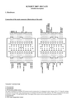
Contents
ABSTRACT ...........................................................................................................................4
INTRODUCTION.................................................................................................................5
PART I - STATE OF THE ART
CHAPTER 1
THEORY AND APPLICATION OF CONDUCTIVITY.....................................................8
1.1 UNITS OF CONDUCTIVITY............................................................................................10
1.2 CONCEPT OF THE CELL CONSTANT ..............................................................................12
1.3 TEMPERATURE EFFECTS..............................................................................................15
1.4 POLARISATION ............................................................................................................19
1.5 TOTAL DISSOLVED SOLIDS (TDS) ..............................................................................19
1.6 ALTERNATIVE MEASUREMENT TECHNOLOGIES ..........................................................19
1.6.1 Contacting conductivity ......................................................................................19
1.6.2 Toroidal (Inductive) conductivity .......................................................................21
1.7 SOURCES OF ERROR IN MEASUREMENT ........................................................................22
1.7.1 Temperature Compensation................................................................................22
1.7.2 Improper Calibration..........................................................................................23
1.7.3 Condition of Probe..............................................................................................23
CHAPTER 2
THE INDUCTIVE CONDUCTIVITY SENSOR ..............................................................24
2.1 THE EXACT THEORY OF INDUCTIVE CONDUCTIVITY SENSORS ...................................24
2.1.1 The Single Transformer ......................................................................................25
2.1.2 The Double Transformer ....................................................................................28
2.2 THE INDUCTIVE CONDUCTIVITY CELL FOR WATER SALINITY MONITORING ..................31
2.2.1 Sensor design ......................................................................................................31
2.2.2 Sensor modelling.................................................................................................32
2.2.3 Experimental characterization ...........................................................................35
PART II - THE PROPOSAL
CHAPTER 3
GENERAL DESCRIPTION OF THE WIRELESS CONDUCTIVITY SENSING FOR
WATER SALINITY MONITORING .................................................................................37
3.1 GENERAL ARCHITECTURE OF WIRELESS CONDUCTIVITY SENSING..............................37
3.1.1 Hardware architecture .......................................................................................37
1
3.2 GENERAL ARCHITECTURE OF OSCILLATOR .................................................................42
3.2.1 Requirements for Oscillation ..............................................................................43
3.2.2 Phase Shift in the Oscillator ...............................................................................45
3.2.3 Gain in the Oscillator .........................................................................................47
3.2.4 Effect of the Active Element (Op Amp) on the Oscillator ...................................47
3.2.5 Analysis of Oscillator Operation (Circuit) .........................................................49
3.2.6 Sine Wave Oscillator Circuits.............................................................................51
3.3 MICROCONTROLLERS DESIGNER .................................................................................53
3.3.1 Microcontrollers choice......................................................................................55
3.4 INTELLIGENT RF MODULE ...........................................................................................56
3.4.1 �One Way’ Easy-Radio for Transmitters & Receivers........................................57
3.4.2 �Two Way’ for Transceivers ...............................................................................59
3.4.3 RSSI - Received Signal Strength Indicator .........................................................62
PART III - IMPLEMENTATION
CHAPTER 4
HARDWARE INDUCTIVE SENSOR INTERFACE.......................................................63
4.1 ELECTRICAL CIRCUIT OF THE HARDWARE INDUCTIVE SENSOR INTERFACE .................64
4.1.1 Quadrature Oscillator & operational amplifier TL082C...................................66
4.1.2 Analog Multiplier - AD633 .................................................................................69
4.1.3 Low-pass Filters .................................................................................................73
4.1.4 Connectors ..........................................................................................................75
4.2 BUILDING PCB HARDWARE SENSOR INTERFACE .........................................................76
4.3 BILL OF MATERIALS 1В° PCB........................................................................................78
CHAPTER 5
HARDWARE REMOTE NODE AND INTERFACE CCP SERVER..............................80
5.1 ELECTRICAL CIRCUIT OF THE NODE ............................................................................80
5.1.1 Microcontroller 18F458 .....................................................................................83
5.1.2 Temperature Sensor AD22103...........................................................................88
5.1.3 Analog input and A/D conversion.......................................................................92
5.1.4 Digital Potentiometer – AD7376 ........................................................................94
5.1.5 DIP Switch ........................................................................................................100
5.1.6 Connection PIC18F458 - RF transceiver.........................................................101
5.1.7 Antenna .............................................................................................................106
5.1.8 Voltage regulator..............................................................................................108
5.1.9 Connectors ........................................................................................................110
5.2 BUILDING PCB NODE ................................................................................................111
5.3 BILL OF MATERIALS 2В° PCB......................................................................................112
5.4 ELECTRICAL CIRCUIT OF THE CCP INTERFACE ..........................................................115
5.4.1 Bridge RF transceiver - Max232 – RS232 port ...............................................117
5.4.2 Voltage regulator..............................................................................................118
5.5 BUILDING PCB MASTER SERVER ...............................................................................119
2
5.6 BILL OF MATERIALS 3В° PCB......................................................................................120
PART IV - EXPERIMENTAL RESULTS
CHAPTER 6
TESTING AND CHARACTERIZATION OF THE INDUCTIVE SENSOR................122
6.1 THE LOW-COST TEMPERATURE CONTROLLED SYSTEM: SYSTEM DESCRIPTION ........122
6.1.1 The container ....................................................................................................123
6.1.2 Heating/cooling thermoelectric pump ..............................................................124
6.1.3 Measuring System .............................................................................................125
6.1.4 PID controller...................................................................................................126
6.2 EXPERIMENTAL CHARACTERIZATION ........................................................................127
6.2.1 Experimental setup ...........................................................................................127
6.2.2 Experimental Characterization and Discussion ...............................................129
CONCLUSIONS ...............................................................................................................136
APPENDIX A....................................................................................................................137
MPLAB IDE...................................................................................................................137
APPENDIX B....................................................................................................................142
C18 C COMPILER ............................................................................................................142
APPENDIX C....................................................................................................................143
ALTIUM DESIGNER 6.......................................................................................................143
APPENDIX D...................................................................................................................145
EASY-RADIO SOFTWARE AND CONFIGURATION COMMAND SET ....................................145
BIBLIOGRAPHY .............................................................................................................150
3
Abstract
This thesis presents the development of a conductivity sensing network based on wireless
transmission. The architecture of the system includes two sensors (inductive conductivity
and temperature), a first PCB (Hardware Inductive Sensor Interface) that drives the
inductive sensor with a sinusoidal oscillator and extracts the DC-signal components in
phase and quadrature of the inductive sensor output voltage, a second PCB where a
temperature sensor, a processing and communication unit, (18F458 microcontroller), and
a RF transceiver for wireless communication is mounted and a third PCB where is
mounted the RF transceiver used as interface with the central control and processing unit
(CCP) monitoring the data. The experimental data proves that is possible to measure the
electrical conductivity of the salty water by using the projected remote system.
4
Introduction
Water Quality (WQ) monitoring of rivers and seas represents an important task of life
quality assessment. The main parameters associated with the water quality assessment
tasks can be classified in three categories: physical parameters (temperature, pH, dissolved
oxygen, turbidity, conductivity), chemical parameters (heavy metal concentration, nitrate
and phosphorous concentration) and biological parameters (algae and bacteria). The WQ
physical parameters, usually measured by using multiparameter measurement systems,
play an important role on the chemical and biological process in the surface and ground
waters.
The parameters of the water analyzes are the conductivity and the temperature. In this case,
the salinity of the water inside estuary, where the salty tide meets the fresh water current,
may be measured by using conductivity sensors, because the electric conductivity is
directly related to salt content in the water.
For measuring the conductivity of electrolytic solutions, there are, in principle, two groups
of sensors:
1) classical conductivity cells containing two or more electrodes;
2) inductive conductivity sensors containing one or two transformers.
In the sea and rivers the presence of biological organisms and the continuous deposition of
inorganic materials carry to choice the second type of sensors (inductive conductivity
sensors) because the utilization of nude electrodes is especially vulnerable fouling, in fact
the conductance between electrodes is very sensitive to the depositions on their surface.
The inductive sensors present the advantage of a non-direct contact between the sensors
elements and the medium under test [1]. This characteristic allows this type of sensor to be
used for water salinity monitoring.
In this work of thesis the project and construction of the first prototype of a single remote
node for the measurement of the conductivity and temperature of the water based on
wireless transmission will be presented. The system structure offers the possibility to add,
5
INTRODUCTION
without hard investments, other water quality measuring capabilities (e.g. pH, dissolved
oxygen).
The remote nodes will be used to the water salinity monitoring of the Tagus river in Lisbon
(Portugal) near the estuary. In Figure 1 is shown the map of the Tagus estuary.
Figure 1 - Map of the Tagus estuary
In the first chapter the theory and application of conductivity will be described, in
particular the different type of the sensors to measure the conductivity, the temperature
effect, and the sources of error in measurement.
In the second chapter the inductive sensor used in this project will be described, this
inductive sensor has been developed at the Instituto de Telecomunicações (it) of Lisbon, in
a particular way the exact theory of inductive conductivity and the sensor design.
In the third chapter the general characteristics of Conductivity Sensing Network Based On
Wireless Transmission will be described with particular attention to the hardware
6
INTRODUCTION
architecture as the Oscillator, Microcontrollers and the RF module used to develop the
main functionalities of the Remote Water Quality Monitoring System.
In the fourth chapter the project and construction of a first PCB (Printed Circuit Board)
called Hardware Sensor Interface used to drive an inductive conductivity sensor for water
salinity monitoring will be presented. The sensor used is an inductive conductivity sensor
described in the second chapter. The PCB has the following functions: 1) driving the
inductive sensor by a sinusoidal oscillator. This oscillator has two outputs with exactly
equal amplitudes but with a phase difference of ПЂ/2; 2) by using multipliers and convenient
signal conditioning, the amplitudes of the components in phase and of phase ПЂ/2 of the
sensor output are obtained in the form of two DC-signals.
In the fifth chapter the second PCB where is mounted a temperature sensor, a processing
and communication unit (18F458 microcontroller) and a RF transceiver for wireless
communication and a third PCB, where is mounted the RF transceiver with the PC master
server for monitoring the data will be presented.
In the sixth chapter the testing and the characterization of the node with the inductivity
conductivity sensor mounted on the first PCB will be presented. A low cost testing bath
with automated controlled temperature to characterize sensors for in-situ water quality
monitoring building in IT laboratories will be used.
7
Chapter 1
Theory and Application of Conductivity
Conductivity (or Electrolytic Conductivity) is defined as the ability of a substance to
conduct electrical current. It is the reciprocal of the resistivity [2].
In water, it is generally used as a measure of the mineral or other ionic concentration.
Conductivity is a measure of the purity of water or the concentration of ionized chemicals
in water. However, conductivity is only a quantitative measurement: it responds to all ionic
content and cannot distinguish particular conductive materials in the presence of others.
Only ionizable materials will contribute to conductivity; materials such as sugars or oils
are not conductive.
In a metal conductor, electrical current is the flow of electrons and is called electronic
conductance. In water, electrical current is carried by ions since electrons do not pass
through water by themselves. This is electrolytic conductance.
When a voltage is applied between two inert electrodes immersed in a solution, any ions
between them will be attracted by the electrode with the opposite charge. Ions will move
between electrodes and produce a current depending on the electrical resistance of the
solution. This is the basis of conductivity measurement - an application of Ohm’s law
(show Figure 1.1). For high purity waters, it is common to express conductivity as its
reciprocal, resistivity.
8
CHAPTER 1
THEORY AND APPLICATION OF CONDUCTIVITY
Figure 1.1 - Using Ohms Law , V= iR and knowing conductivity G = 1/R then
G can be determined as G= 1/R = i/V
To prevent altering the sample by major ionic movement and electrochemical reaction at
the electrodes, alternating current is always used for measurement. With AC the polarity
changes frequently enough that ions do not move or react significantly. Measuring systems
must control the voltage, frequency and current density to minimize errors due to electrode
polarization and capacitance. Modern instrumentation may change one or more of these
variables automatically, depending on the conductivity range being measured.
In the chemical water treatment field our interest is in measuring the conductivity of waters
which consist of ionic compounds dissolved in the water.
This conductivity is quite easily measured by electronic means and this offers a simple test
or control level which can tell much about the quality of the water.
Conductivity of very dilute solutions can be calculated from physical chemistry data based
on Equation 1.1 which sums the conductivity contribution of all ions in the solution [4].
Пѓ = ПЃ * ОЈ (О»i * ci)
Пѓ = conductivity
ПЃ = density of water
λi = equivalent ionic conductance of ion �i’
c i = concentration of ion �i’
9
(1.1)
CHAPTER 1
THEORY AND APPLICATION OF CONDUCTIVITY
1.1 Units of Conductivity
The basic unit of resistance is the ohm, - conductance is the reciprocal of resistance and its
basic unit is the siemens, formerly called the mho [2].
In discussions of bulk material it is convenient to talk of its specific conductance, or more
commonly called its conductivity.
Conductivity is the conductance as measured between the opposite faces of a 1- cm cube of
the Material (show Figure 1.2) .
Figure 1.2 – cell constant = 1 cm electrode spacing divided by 1 cm2 cross-sectional area of sample
This measurement has units of Siemens/cm. More common in water treatment the units
ОјS/cm (microsiemens) and mS/cm (millisiemens) are used as they are more meaningful.
The corresponding terms for specific resistance (or resistivity) is ohm-cm, megohm-cm
and kilohm-cm.
Measurement
Resistance
Conductance
Resistivity
Conductivity
Application
Electrical circuit
Electrical circuit
High purity water
Most water samples
Units
Ohm (О©)
ohm-1 (О©-1) = siemens (S) = mho (now obsolete)
Ohmв‹…cm (О©в‹…cm)
siemens/cm (S/cm) = mhos/cm (now obsolete),
siemens/m (S/m)*
* Most users employ units of S/cm. However, SI conductivity units used in some parts of the world are S/m
which can easily be confused. 1 S/cm = 100 S/m.
Review the following tables for typical conductivity of the water at the temperature of
25В°C [5]
10
CHAPTER 1
THEORY AND APPLICATION OF CONDUCTIVITY
table 1.1 – Typical conductivity of the water at the temperature of 25 °C
A conductivity measurement responds to any and all ions present in a solution. A solution
cannot be identified, or its concentration known, from conductivity alone (see Figure 1.3).
In certain cases, the concentration of an electrolyte in solution can be determined by
conductivity if the composition of the solution is known [6].
11
CHAPTER 1
THEORY AND APPLICATION OF CONDUCTIVITY
Figure 1.3 - A solution cannot be identified from conductivity alone
1.2 Concept of the cell constant
In theory, a conductivity measuring cell is formed by two 1-cm square surfaces spaced 1cm apart. Cells of different physical configuration are characterized by their cell constant,
Kc. This cell constant (Kc) is a function of the electrode areas, the distance between the
electrodes and the electrical field pattern between the electrodes [3].
A cell for measuring conductivity may be made up as shown in the Figure 1.4, it is made
of insulating material except for the opposite faces A and B which are made of metal. If it
is filled with a conductivity solution L, the conductance measured between the faces A and
B is the following:
G = L A/ l
where
G = conductance in Siemens
L = Conductivity in Siemens/cm
l = distance in cm between the electrodes or faces A and B
A = surface in cm2 perpendicular to the flow of current.
12
CHAPTER 1
THEORY AND APPLICATION OF CONDUCTIVITY
Figure 1.4 - A cell for measuring conductivity
The corresponding equation for the resistance is:
R = ПЃ l /A
where
R = resistance in ohm
ПЃ = resistivity in ohm*cm
l = distance in cm between the electrodes
A = surface in cm2 perpendicular to the flow of current.
The term l /A is defined as Kc, the cell constant of resistivity, and its measuring unit is the
cm-1.
Conductivity Cell Constant =
в€’1
Length
1 cm
=
= 1cm
2
Area
1 cm
The cell constant of the resistivity is used for all the applications, irrespective of whether
conductivity or resistivity is being used: the result is
G = L/Kc or KcG = L
For example, for an observed conductance reading of 200 ВµS using a cell with Kc 0. 1, the
conductivity value is 200 x 0. 1 = 20 ВµS/cm [5].
As the dimensions of the cell change, the cell constant varies with the ratio l /A (show
Figure 1.5).
13
CHAPTER 1
THEORY AND APPLICATION OF CONDUCTIVITY
(a)
(b)
Figure 1.5 – (a) 0.1 constant; (b) 10.0 constant
Cell constants other than 1 cm-1 may be used as long as the measuring instrument readout
is normalized accordingly. A lower cell constant sensor is needed to enable the measuring
instrument to make accurate measurements in low conductivity (high resistivity) samples.
Higher cell constants are needed to measure in high conductivity samples. The exact
requirements depend on the measuring instrument.
In a simplified approach, the cell constant is defined as the ratio of the distance between
the electrodes, l, to the electrode area, A. This however neglects the existence of a fringefield effect, which affects the electrode area by the amount AR. Therefore Kc = l/(A + AR).
Because it is normally impossible to measure the fringe-field effect and the amount of AR
to calculate the cell constant, Kc, the actual Kc of a specific cell is determined by a
comparison measurement of a standard solution of known electrolytic conductivity.
The most commonly used standard solution for calibration is 0.01 M KCl. This solution
has a conductivity of 1412 ВµS/cm at 25oC
In summary, the calibration of a conductivity probe is to compensate for the fact that:
•
Kc is not specifically known
•
Kc changes as the electrode ages
Calibration simply adjusts the measured reading to the true value at a specified temperature
[3].
In order to produce a measuring signal acceptable to the conductivity meter, it is highly
important that the user choose a conductivity electrode with a cell constant appropriate for
14
CHAPTER 1
THEORY AND APPLICATION OF CONDUCTIVITY
his sample. The table below lists the optimum conductivity range for cells with different
cell constants.
Cell Constant Optimum Conductivity Range
0.01
0.055 - 20 ОјS/cm
0.1
0.5 - 200 ОјS/cm
1.0
0.01 - 2 mS/cm
10.0
1 - 200 mS/cm
table 1.2 – Lists the optimum conductivity range for cells with different cell constants
1.3 Temperature Effects
Conductivity is affected by temperature since water becomes less viscous and ions can
move more easily at higher temperatures. Conventionally, conductivity measurements are
referenced to 25 В°C though occasionally a 20 В°C reference is used [3]. The variation with
temperature is apparent in Equation 1.1 since О»i, and to a lesser degree, ПЃ are temperature
dependent. The conductivity of most ions increase in conductivity by about 2.2% of their
value per В°C which allows for simple temperature compensation. This is suitable for most
mid-range conductivity measurements. Very low and very high conductivity samples
require special handling of temperature effects.
In moderately and highly conductive solutions, this increase can be compensated for using
a linear equation involving a temperature coefficient (О±), which is the percent increase in
conductivity per degree centigrade (see Figure 1.6).
The degree to which temperature affects conductivity varies from solution to solution and
can be calculated using the following formula:
CT = CTcal [1 + О±(T-Tcal)]
where:
15
(1.2)
CHAPTER 1
THEORY AND APPLICATION OF CONDUCTIVITY
CT = conductivity at any temperature T in В°C;
CTcal = conductivity at calibration temperature Tcal in В°C;
О± = temperature coefficient of solution at Tcal in В°C.
The temperature coefficients of the following electrolytes generally fall in the ranges
shown below:
Substance at 25В°C
Alpha (О±)
Acids
1.0 - 1.6%/В°C
Bases
1.8 - 2.2%/В°C
Salts
2.2 - 3.0%/В°C
Fresh water
2.0%/В°C
For example, by definition, temperature compensated conductivity of a solution is the
conductivity which that solution exhibits at the reference temperature. This temperature is
chosen to be either 25 oC or 20 oC. A measurement made at reference temperature,
therefore, needs no compensation. Generally for most aqueous samples, a coefficient of
2.1% per degree Celcius is used in temperature compensation, with the apparent value
being 2.1% high for each degree C above 25 oC or conversely the apparent value being
2.1% low for each temperature for measurement is 25 oC. Using the formula (1.2):
CT = C25 [1 + 0.021 (T - 25)]
To determine that О± of other solutions, simply measure conductivity at a range of
temperatures and graph the change in conductivity versus the change in temperature.
Divide the slope of the graph by CTcal to get О±.
16
CHAPTER 1
THEORY AND APPLICATION OF CONDUCTIVITY
Figure 1.6 - Temperature Compensation for Conductivity Increase with Temperature
For example in Figure 1.6 is show the conductivity vs temperature for a generic solution
[6]. To calculate the temperature coefficient (О±) to be input into a conductivity analyzer,
simply:
1. Divide the temperature slope(s):
вЋЎ 60-30mS/cm вЋ¤
S= вЋў
вЋҐвЋ¦ = 1.20
50 - 25 В°C
вЋЈ
2. By the conductivity at 25В°C, C(25В°C):
S
1.2
=
= 0.040
o
C(25 C) 30
3. and multiply by 100:
О± = 100 (.040) = 4.0%
All meters have either fixed or adjustable automatic temperature compensation referenced
to a standard temperature - usually 25В°C. Most meters with fixed temperature
compensation use a a of 2%/В°C (the approximate a of NaCl solutions at 25В°C). Meters with
adjustable temperature compensation let you to adjust the a to more closely match the a of
your measured solution.
A very modern technique uses a microprocessor and an associated "look up" table which
contains the temperature response of the solution. The solution temperature is measured
17
CHAPTER 1
THEORY AND APPLICATION OF CONDUCTIVITY
and converted to digital form, from this information and data in the "look up" table a very
accurate temperature compensation can be derived.
Note the two following examples to explain the effect and compensation of the fringe-field effect and
temperature.
Example #1 - Manual Temperature Compensation:
An analyst wishes to calibrate a conductivity probe and measure an unknown sample. The conductivity probe
is specified to have a cell constant of 1.0. The analyst is calibrating in a 0.01 M KCI (EC = 1412 ВµS/cm at
25oC) solution at a temperature of 22oC. Automatic temperature compensation (ATC) is not available.
1.
2.
Determine the conductivity of the 0.01 M KCI at 22oC.
o
EC KCI 22oC = 1412[l + 0.021(22-25)]
o
EC KCI 22oC = 1412 [0.937]
o
EC KCI 22oC = 1323 ВµS/cm
Immerse the conductivity probe into the standard and adjust the value to 1323 ВµS/cm. adjustment
being made is compensating for the difference the specified cell constants and the true cell constant.
3.
The analyst now measures an unknown sample whose temperature is at 19oC and obtains a value of
967 ВµS/cm. How is this value adjusted to 25oC
967 ВµS/CM = C25[1 + 0.021(19-25)]
C25 = 967 ВµS / [1 + 0.021(19-25)]
C25 = 967 ВµS / [1 + 0.021(-6)]
C25 = 967 ВµS / 0.874
C25 = 1106 ВµS/cm
Example #2 - Automatic Temperature Compensation:
An analyst wishes to calibrate the conductivity probe and measure a sample. The conductivity probe is
specified to have a cell constant of 1.0. The analyst is calibrating in a 0.01 M KCI (EC = 1412 ВµS/cm at
25oC) solution at a temperature of 22oC. Automatic temperature compensation (ATC) at 25oC is available.
1.
Immerse the conductivity probe into the standard and adjust the value to 1412 ВµS/cm. Any
adjustment being made is compensating for the difference between the specified cell constants and
the true cell constant. NOTE: On most modern instrumentation, the true temperature is displayed
along with the temperature compensated conductivity value. In this case the display would show a
conductivity of 1412 ВµS/cm and of 22oC.
2.
Once the electrode has been calibrated, it is cleaned, placed into the unknown sample at 19oC. Once
temperature is stable, the correct conductivity value (1106) ВµS is displayed
18
CHAPTER 1
THEORY AND APPLICATION OF CONDUCTIVITY
1.4 Polarisation
Polarisation can cause formation of gas at metallic surfaces even though high frequency
AC is used in measurement, the effect can take place in the half cycle of one polarity.
Another reason is a depletion of anions or cations around the electrode due to the charge
build up. Polarisation is an insidious effect in that conductivity readings can be lower than
the true value but by an unknown amount and a reading is obtained from the instrument
with no indication that it is incorrect. Similar effects are noted if grease or oil are present in
the solution, or if the electrodes are fouled or scaled in any way. Polarisation can be
reduced by using high frequency AC, keeping the current density low by the correct choice
of cell constant and by making surfaces rough such as graphite, and by operating in
conductivities of less that 30,000 ОјS/cm, and in the case of fouling, by removal of the
sensor and cleaning frequently [2].
1.5 Total Dissolved Solids (TDS)
TDS is sometimes inferred from conductivity and is reported in units of parts per million.
However, the relationship of conductivity and concentration is not standardized and to be
meaningful, should be specified whenever TDS units are used. Typical conversions are
based on sodium chloride (which may also be called salinity) at approximately 0.5 ppm
TDS per μS/cm. Alternatively, a “natural water” mineral composition including
bicarbonates would have a conversion of 0.6 – 0.7 ppm TDS per μS/cm. Conversions may
also be slightly non-linear with concentration.
1.6 Alternative Measurement Technologies
1.6.1 Contacting conductivity
In Figure 1.1 and its description above refer to the conventional two-electrode sensor and
measurement technique.
Most practical cells do not use the parallel plate electrode arrangement of Figure 1.1. They
have greater durability and allow more convenient installation with other arrangements.
19
CHAPTER 1
THEORY AND APPLICATION OF CONDUCTIVITY
For example, typical pure water sensors for on-line measurement use concentric electrodes
that maintain the spacing and geometry for 0.01 to 0.1/cm constant. A variety of twoelectrode process conductivity sensors is illustrated in Figure 1.7.
Figure 1.7 – Conventional two-electrode conductivity sensors: 0.1 cm-1in retractable housing,0.1 cm-1in flow
chamber, sanitary 0.1 cm-1, 10cm-1insertion, 50-1cm insertion, long 0.1cm-1insertion, short 0.1 cm-1insertion.
Four-electrode conductivity measurement uses a sensor incorporating four electrodes. It is
useful for highly conductive and/or dirty water samples which would foul the surfaces or
plug the narrow passages of conventional high constant two-electrode sensors [4].
Four-electrode measurement applies AC through the sample via two outer drive electrodes
as shown in Figure 1.8.
V
Figure 1.8 – Four-electrode conductivity measurement
20
CHAPTER 1
THEORY AND APPLICATION OF CONDUCTIVITY
These electrodes may become fouled and the circuit will compensate to maintain the AC
current level constant. Two inner measuring electrodes are used to sense the voltage drop
through the portion of solution between them. The circuit makes a high impedance AC
voltage measurement, drawing negligible current and making it much less affected by
additional resistance due to fouling of the measuring electrode surfaces. Sensors for four
electrode conductivity measurement are shown in Figure 1.9.
Figure 1.9 – Four-electrode Conductivity Sensors
1.6.2 Toroidal (Inductive) conductivity
Inductive (also known as non-contact, electrodeless or toroidal) conductivity measurement
is made without any direct electrical contact with the sample. The sensor consists of two
parallel coils sealed within a doughnut-shaped insulated probe as shown in Figures 1.10
and 1.11. A transmitting coil generates a magnetic alternating field that induces an electric
voltage in a liquid. The ions present in the liquid enable a current flow that increases with
increasing ion concentration. The ionic concentration is then proportional to the
conductivity. The current in the liquid generates a magnetic alternating field in the
receiving coil. The resulting current induced in the receiving coil is measured and used to
determine the conductivity value of the solution. Advantages to this type of cell are:
•
No polarization
•
Reduced maintenance and resistance to chemical attack
•
Complete galvanic separation of measurement from medium (eliminates ground
loss)
21
CHAPTER 1
THEORY AND APPLICATION OF CONDUCTIVITY
Figure 1.10 – Inductive Conductivity Measurement
Figure 1.11 – Inductive Conductivity Measurement Equipment
1.7 Sources of error in measurement
1.7.1 Temperature Compensation
Since many conductivity probes now include a thermistor for ATC it is important to
determine if the thermistor reading is accurate at the temperatures that samples are being
measured. If not, then the automatic temperature corrected value will be inaccurate.
Compare the measured value from the thermistor with that of a quality laboratory
22
CHAPTER 1
THEORY AND APPLICATION OF CONDUCTIVITY
thermometer. If the values differ significantly, contact the manufacturer as to the defect or
consider manual temperature compensation.
1.7.2 Improper Calibration
Too often, calibration standards have been sitting around a laboratory for extended
periods. Standards should be fresh and known to be correct within at least В± 1% before
attempting a calibration. Since the conductometric response is not perfectly linear at all
ranges it is best to calibrate the probe in the same magnitude of range as the samples being
measured. In other words don't calibrate your conductivity probe in a 100 ВµS/cm standard
if your samples are typically in the >1000 ВµS/cm range. Standard conductivity solutions:
Conductivity (mS/cm)1
0.147
1.413
2.767
6.668
KCI Concentration
0.001 N
0.010 N
0.020 N
0.050 N
1
temperature KCl solutions 250C
1.7.3 Condition of Probe
Probes can become inaccurate when they become coated with interfering substances on the
probe element. During normal use, rinse the probe thoroughly with laboratory grade water
between each measurement. This will help to minimize the buildup of the coating
substances. If the probe needs cleaning first try ethanol which is good for removing most
organics. If this isn't successful, clean the probe with a strong detergent solution. Rinse
thoroughly with demineralized water.
The cells may occasionally need replatinization to refresh the cell plates and return them
back to the original cell constant. The cell constant changes when the platinum black layer
becomes partially removed or contaminated. Follow the manufacturer's directions on this
procedure [3].
23
Chapter 2
The Inductive Conductivity Sensor
Besides temperature and pressure, conductivity is among the most relevant parameters
characterizing the physical (thermodynamical) state of seawater.
For measuring the conductivity of electrolytic solutions, there are, in principle, two groups
of sensors (As it has been seen in the previous chapter 1):
1) classical conductivity cells containing two or more electrodes;
2) inductive conductivity sensors containing one or two transformers.
In oceanographic work this type of sensors has found broad application [1].
In this experimental project the second sensor will be used and, for this reason, it is better
to illustrate in detail the exact theory of inductive conductivity sensors derivated by Klaus
Striggow and Reinhard Dankert in the 1984 [7].
2.1 The Exact Theory of Inductive Conductivity Sensors
As is well known, inductive sensors have the advantage that there are no electrodes, which
suffer from polarization and fouling thereby preventing long-term stability [8]. But, there is
a new problem caused by the variability of the permeability of the transformer core(s) due
to its temperature and pressure dependence. During in situ measurements, temperature and
pressure can often quickly vary over the intervals -2°C ≤T ≤ 30°C and 0 ≤ p≤ 108 Pa. As is
shown in Figure 2.1, the permeability of transformer-core materials is a nonlinear function
of T and p which, additionally, is influenced by relaxation and hysteresis.
24
CHAPTER 2
THE INDUCTIVE CONDUCTIVITY SENSOR
(a)
(b)
Figure 2.1 - Dependence of the normalized permeability u/u(0,0) of transformer core materials on: (a)
temperature T and (b) pressure P. u(0, 0) is the initial value of the permeability in a temperature pressure
cycle. Pay attention to nonlinearity, relaxation, and hysteresis. (Muniperm is a metallic material, Manifer
110 and 150 are ceramic core materials produced by VEB Keramische Werke HermsdorfiThiir. Magnetic
materials of other producers may not be expected to have less complicated properties.)
In this project the pressure dependence of the permeability is not important because the
remote node of the sensors is dislocated only up the river and not at down level. For the
temperature there aren’t problem again with the permeability effect because the
temperature of the water in the Tagus estuary is surely between the intervals -2°C ≤ T ≤
30В°C
The exact theory of inductive conductivity sensors for oceanographic, that now it is being
described, will be based on two commonly used types of inductive conductivity sensors:
•
single transformer;
•
double transformer.
2.1.1 The Single Transformer
The simplest form of the inductive conductivity sensor for a liquid is a transformer, the
secondary coil of which is formed by the surrounding liquid, here the seawater (see Figure
2.2). The primary current is then the sensor output signal.
25
CHAPTER 2
THE INDUCTIVE CONDUCTIVITY SENSOR
Figure 2.2 - The single transformer as conductivity sensor: construction. (G: case, K: ringshaped core of the
transformer, l: primary coil of the transformer, M: seawater loop (= secondary coil)).
The relationship who exists between the resistance Rw, of the seawater loop and the sensor
output I1 is:
вЋ› 1
1 вЋћ
I1 = вЋњ 2 +
вЋџ U1
⎝ n1 Rw jω L11 ⎠(2.1)
where:
n1 is the number of windings;
L11 the inductance of the (primary) coil;
j=
в€’1 , П‰ = 2ПЂf, and f the frequency.
The circuit of the Figure 2.2 is show in Figure 2.3 (a). Equation (2.1) directly leads to the
equivalent circuit (see Figure 2.3(b)) of this type of sensor.
(a)
(b)
Figure 2.3 – (a) circuit, (b) equivalent circuit.
26
CHAPTER 2
THE INDUCTIVE CONDUCTIVITY SENSOR
Furthermore, it makes evident that the primary current I1 consists of two components:
-
the real or active component
Ilact = [1/(n12Rw)]Ul
being in phase with the primary voltage Ul,
-
and the imaginary component
Ilimg = [(l/(jωLl1]U1
being in quadrature to the primary voltage.
Obviously Ilact is a function of Rw alone, and not of the inductance L11. Therefore the real
component of the primary current is a measure of the conductivity, independent of
permeability of the core! Although this configuration is very simple it has not been applied
to oceanographic conductivity sensors.
There are several methods available to determine the active component Ilact of the primary
current I1:
1) The peak value Iˆ1 , of the primary current Il, as well as its phase shift φ against the
primary voltage Ul are measured (Figure 2.4).
Figure 2.4 – Primary current if the primary voltage is sinusoidal
Then the peak value Iˆ1act of the active component can be calculated by
Iˆ1act = Iˆ1 cos ϕ
2) The peak value Iˆ1act of the active component is measured directly by sampling the
primary current exactly at that moment when the primary voltage passes its maximum
(Figure 2.4).
27
CHAPTER 2
THE INDUCTIVE CONDUCTIVITY SENSOR
3) The peak or mean value oft he active component of the primary current is measured by
means of a wattmeter.
4) The sensor is shunted with a capacitance C. Based on the equivalent circuit of the sensor
(Figure 2.3b) and ( 2.l ) , the total input current is
вЋ› 1
вЋћ
1
+ jωC ⎟ U1
I1total = вЋњ 2 +
⎝ n1 Rw jω L11
вЋ (2.2)
By choosing C so that П‰C = 1/(П‰L11), the reactive or imaginary component vanishes, and
Iltotal becomes an exact measure for Rw.
5) The sensor is designed in such a manner that the condition П‰L11 >> n12 Rw is satisfied.
Then, according to (2.1) , the imaginary component becomes sufficiently small and the
primary current becomes an approximative measure of Rw.
2.1.2 The Double Transformer
The double transformer is used for measuring the conductivity of liquids and is widely
applied to oceanographic instrumentation.
The double transformer consists of two transformers where a water loop forms both the
secondary coil of the first transformer (“driver transformer”) and the primary coil of the
secondary transformer (“pickup transformer”) (see Figure 2.5(a) and (b)).
(a)
28
THE INDUCTIVE CONDUCTIVITY SENSOR
CHAPTER 2
(b)
Figure 2.5 – The double transformer as conductivity sensor: (a) construction and (b) circuit. (K1, K2: ringshaped cores oft he first and second transformer, 1, 4: primary coil of the first and secondary coil of the
second transformer, M: seawater loop ( = secondary coil of the first as well as primary coil
of the second transformer)).
It is important to arrange the two transformers in such a manner that the only coupling
between them is by the common water loop.
The voltage or current of the second coil of the pickup transformer is considered as the
sensor output signal.
The relationship between Rw and U4 is:
U4 =
n4
n1
1
U1
вЋ› 1
1 вЋћ
2
1 + n4 Rw вЋњ
+
вЋџ
⎝ RA jω L44 ⎠(2.3)
Up to now, oceanographic applications have taken advantage of three special cases
involving (2.3).
1) The short-circuit current I4,K is a measure of Rw which is independent of the
inductance L44, i.e., the permeability. Indeed, from (2.3) it follows that:
I 4,k = lim (U 4 / RA ) =
RA в†’ 0
29
1
U1
n1n4 Rw
(2.4)
CHAPTER 2
THE INDUCTIVE CONDUCTIVITY SENSOR
2) Used a very small terminating resistor RA satisfying the condition RA << П‰L44. In
this special case, according to (2.3), U4 becomes nearly independent of L44.
3) Shunted the terminating resistor RA with a capacitor C in their instrument. Then in
(2.3) the term 1/RA must be substituted by ((l/RA) + jωC). If C satisfies the
condition ωC ≈ l/(ωL44), the imaginary terms within the bracket cancel, and U4
becomes (nearly) independent of L44.
The (2.3) reveals further possibilities for eliminating the unwanted effect of shifting
permeability. After transformation to the equivalent form
U1 =
n1 вЋ› n4 2 Rw jn4 2 Rw вЋћ
в€’
вЋњ1 +
вЋџU
n4 вЋќ
RA
П‰ L44 вЋ 4
(2.5)
(2.3) allows the following interpretation. U1 can be decomposed into two components, the
first of which
n1 вЋ› n4 2 Rw вЋћ
вЋњ1 +
вЋџU 4
n4 вЋќ
RA вЋ is in phase with U4 and independent of permeability, whereas the second
вЋ› jn1n4 Rw вЋћ
вЋњв€’
вЋџU 4
⎝ ω L44 ⎠has a phase lag of 90” relative to U4, and depends on L44. This directly leads to the
following methods.
4) U1 and U4 are sampled when the latter passes its maximum. Because at this
moment the quadrature component ( - j … U4) crosses zero, it follows from (2.5)
that
U1* =
n1 вЋ› n4 2 Rw вЋћ Л†
вЋњ1 +
вЋџU 4
n4 вЋќ
RA вЋ (2.6)
where U1* denotes the measured momentary value of U1. This equation allows the
determination of Rw independent of perrneability.
30
CHAPTER 2
THE INDUCTIVE CONDUCTIVITY SENSOR
5) The peak values of both U1, and U4 are sampled as well as the phase angle П†
between them. After having calculated U1* = Uˆ1 cos φ , Rw can be determined as
described under 2.4).
6) U1, and U4 are brought to an averaging multiplier. Then according to (2.5) we find
2
U1 =
n1 вЋ› n4 2 Rw вЋћ
вЋњ1 +
вЋџ U1U 4
n4 вЋќ
RA вЋ (2.7)
Where the bar denotes time averaging. This equation again is independent of
permeability.
2.2 The inductive conductivity cell for water salinity
monitoring
In these paragraphes an inductive sensor constructed as a double transformer is describe, to
be utilized to measure the water salinity in the sea and estuaries. This inductive sensor has
been developed at the Instituto de Telecomunicacoes of Lisbon [9].
2.2.1 Sensor design
The sensor structure is shown in Figure 2.6. Two toroidal cores of amorphous iron are
mounted together as shown in Figure 2.6. Each core is provided with one winding of 20
turns. This assemble is immersed in the aqueous solution. A plastic container is used to
delimit the lines of current inside the water, preventing the influence of strange objects on
the measuring process. Therefore all the current in the water is enclosed by the plastic
container. However, the container is provided with some apertures to let the water flow
through the cell. The expected lines of current are depicted in the Figure 2.7.
31
CHAPTER 2
THE INDUCTIVE CONDUCTIVITY SENSOR
Figure 2.6 - Cell structure: two cores with one winding each inside a plastic container.
42
13
40
136
22
Figure 2.7 - Lines of current embracing the two toroids inside the plastic container.
The dimensions are in millimeters.
The cell will work in an alternate sinusoidal regime. However, the resistance of the water
path may be calculated assuming stationary fields, if the depth of penetration Оґ in the water
is much greater than the cell dimensions for the maximum frequency of operation.
Considering the maximum frequency as f max = 50 kHz and Пѓ max = 5 S/m we obtain using
(2.8), a value for the depth of penetration of the order of one meter. This will guarantee
that the depth of penetration of the electromagnetic field in the salty water will always be
greater than the dimensions of the sensor, for the entire range of the conductivities to be
measured.
Оґ min =
2
П‰max Ој0Пѓ max
(2.8)
2.2.2 Sensor modelling
The finite element method was used to estimate the configuration of the electric field
induced inside the cell. As shown in the previous section the current field can be
32
CHAPTER 2
THE INDUCTIVE CONDUCTIVITY SENSOR
determined as in the dc-regime. Equipotentials and lines of current were determined using
this method. The lines of current are shown in the Figure 2.8. These results allow the
determination of the water resistance and of the cell constant. This modeling shows that the
resistance RW of the water path may be written in the form,
RW =
KC
Пѓ
(2.9)
where KC is the cell constant, which only depends on the geometric shape. In our case and
for the linear dimensions presented on the Figure 2.7 the value KC = 110 m-1 was obtained.
Figure 2.8 - Current lines obtained using the finite element method.
The electric circuit represented in Figure 2.9 is useful to preview the electric behavior of
the presented sensor. However in this scheme the dispersion of the magnetic field lines and
the resistance of the wire windings are neglected. The effect of parasitic capacitances is not
taken into account.
Figure 2.9 - Sensor schematic circuit: RW represents the resistance of the water circuit.
The circuit represented in Figure 2.9 has an equivalent as represented in Figure 2.10. The
first transformer is represented by the electric circuit as seen from the primary (the winding
of 20 turns) and the second transformer as seen from the secondary (20 turns output). In
this equivalent circuit Z represents the impedance of the 20 coils around one toroidal core.
It was verified by measurement that, at the frequency of 50 kHz, the impedance Z
presented an important real part with an angle of losses greater than ПЂ / 4 . However, the
frequency of 50 kHz was chosen because the sensibility increases with frequency. It was
33
CHAPTER 2
THE INDUCTIVE CONDUCTIVITY SENSOR
also verified that the impedance Z did not present important variations for input amplitude
voltage variations between 5 and 10 volt.
Figure 2.10 - Equivalent circuit of the double transformer sensor.
With this model it was possible to preview the behavior of the sensor when it was driven
by a constant voltage source or when it was driven by a constant current source. For a
voltage of imposed constant amplitude applied to the input transformer the expected output
voltage phasor will be
U out = U in
Z
Z + n 2 RW
(2.10)
A close examination of the expression (2.10) shows that the expected sensitivity of the
output voltage to the water resistance RW varies largely in the range of measurement:
dU out
в€’ Zn 2U in
=
dRW
( Z + n 2 RW )2
(2.11)
Being the range of the conductivity measurement (100 mS/m < Пѓ < 5 S/m) , and taking the
equation (2.9) into account, the corresponding values of the water resistance RW will be in
U =1 V
the interval (1.1 kО© > RW > 22 О©) . For Z = (3.2в€ 37Вє ) kО© and in
, the sensitivity given by
(2.11) will be in the interval
6, 54 Г—10в€’6 <
dU out
< 9, 64 Г—10в€’3 V/О©
dRW
(2.12)
The sensitivity of the output voltage to the conductivity Пѓ , also for unitary input voltage,
will be given by
dU out
dU out dRW
=
dПѓ
dRW d Пѓ
which corresponds to the interval
34
(2.13)
CHAPTER 2
THE INDUCTIVE CONDUCTIVITY SENSOR
72 >
dU out
> 42 mV/(S/m)
dПѓ
(2.14)
These results show that the expected absolute errors inherent to the sensor are of the same
order of magnitude, for low or high conductivities, but quite different in relative value.
Therefore a special attention must be taken when projecting the electronic circuitry
associated to the detection of the sensor output voltage.
The sensor is driven by a sinusoidal oscillator working at f=50 kHz and rms output voltage
of Uout=10 V. The components in phase and in quadrature of the sensor output voltage
were measured separately. For a circuit with the topology of that shown in Figure 2.10,
and for the values of Z and U out referred above, the output sensor voltage components will
vary with RW as shown in the Figure 2.11.
1,2
Output Voltages (V)
1
0,8
0,6
0,4
0,2
0
0
100
200
300
400
500
600
700
800
900
1000
Water Resistance (О©)
Figure 2.11 - Cell output voltage. The upper curve is the component in phase and the lower curve
the component ПЂ/2 out of phase with the sensor input.
2.2.3 Experimental characterization
The cell was characterized in a bath of salty water by using an automated set-up previously
developed. The cells were tested varying the frequency and the temperature, in baths of
different salinities. Some of the obtained results are presented in Figure 2.12. These results
show the dependence of the trans-impedance on the frequency, and were used to select the
final frequency of operation for the prototype.
35
CHAPTER 2
THE INDUCTIVE CONDUCTIVITY SENSOR
Transimpedance module for different temperatures
8
|Z21| (О©)
6
20.0 В°C
22.0 В°C
24.0 В°C
26.0 В°C
28.0 В°C
30.0 В°C
4
2
0
0
5000
10000
15000
Frequency (Hz)
20000
25000
30000
Transimpedance phase for different temperatures
180
20.0 В°C
22.0 В°C
24.0 В°C
26.0 В°C
28.0 В°C
30.0 В°C
Phase (Вє)
160
140
120
100
80
0
5000
10000
15000
Frequency (Hz)
20000
25000
30000
Figure 2.12 - Cell transimpedance as a function of frequency and temperature.
The measurements correspond to a solution with conductivity of 43 mS/m at 20.0 ВєC.
Figure 2.12 shows clearly that the sensitivity increases with the frequency. These
measurements were carried out in a bath with conductivity lower than the minimum
conductivity of the measurement range. For this low conductivity value it was possible to
separate the curves measured for different temperatures, and confirm the theoretical law of
variation with the temperature.
36
Chapter 3
General Description of the Wireless
Conductivity Sensing for Water Salinity
Monitoring
In this chapter the general characteristics of the proposed Conductivity Sensing Network
Based On Wireless Transmission will be described with particular attention to the
architecture and to the Oscillator, Microcontrollers and the RF module necessary for the
main functionalities of the Remote Water Quality Monotoring System.
3.1 General architecture of Wireless Conductivity Sensing
3.1.1 Hardware architecture
The Conductivity Sensing Network Based On Wireless Transmission is built as a
master/slave architecture. The remote distributed measuring system includes a node called
primary acquisition and processing units (PAPs). Each PAP contains the hardware
inductive sensor interface, the inductive sensor, the temperature sensor, the processing unit
and the RF module [10]. Communication between the PAPs and the central control and
processing unit (CCP) is based on a RF transmission FSK modulation at 400 MHz or 900
MHz. Thus, the remote node that includes the microcontroller with port USART-RS232
and the RF module can be directly connected to the CCP in order to transmit the numerical
values of water quality parameters from the zones to monitor. In the following two
subsections, two network and communication architectures are presented: a RF – CCP,
which was initially selected for building the first prototype illustrated in this work of
thesis, and a RF – GSM/GPRS which will be developed in future works.
37
CHAPTER 3
GENERAL DESCRIPTION OF WIRELESS CONDUCTIVITY SENSING
FOR WATER SALINITY MONITORING
a) RF wireless transmission architecture
The RF wireless communication is built as a master/slave architecture using the Star
network topology. It is shown in Figure 3.1.
PAP2 unit
PAP3 unit
Central Control and
processing Unit - CCP
Master node
Primary
Acquisition and
Processing unit
– PAP1 unit
PAP4 unit
Slave node
Connection RF
PAPn unit
Figure 3.1 - Network Topology
The wireless connection is based on a direct connection CCP-PAP unit node; all nodes are
directly connected with the CCP. Each node is identified by a node address which
identifies a node in the network in an univocal way.
The type of transmission and receiving with RS232 is serial asynchronous half-duplex,
where a byte is the single unit of transmission with the adding of the start bit and stop bit;
the first bit transmitted is LSB, Least Significative Bit and the velocity of transmission can
arrive at a bound rate of 38400.
In Figure 3.2 is shown the basic idea of the project of the water quality system based on
the RF wireless transmission architecture.
38
CHAPTER 3
GENERAL DESCRIPTION OF WIRELESS CONDUCTIVITY SENSING
FOR WATER SALINITY MONITORING
CCP unit
RS232
Master
RF Transceiver
Directly
connection
Range 250 mt
RF Transceiver
PAP1 unit
RF Transceiver
PAP3 unit
WQ sensors
Water under
test
RF Transceiver
C
T
WQ sensors
PAP2 unit
Slave
Slave
C
T
WQ sensors
C
T
Slave
Figure 3.2 – basic idea of the project
The block diagram of the single PAP and the CCP implemented in the first prototype are
shown in Figure 3.3. The node includes the sensor units, the conditioning circuit and a
microprocessor unit, that establishes the interface between the sensors conditioning circuit
and the transmission unit.
Oscillator
Inductive
Sensor
Sensor
Analog to
Digital
Conversion
Microprocessor
Detection
(a)
39
Low Power
RF
Transciever
CHAPTER 3
GENERAL DESCRIPTION OF WIRELESS CONDUCTIVITY SENSING
FOR WATER SALINITY MONITORING
Low Power
RF
Transciever
RS232
Central
PC
Server
(b)
Figure 3.3 – General architecture of the first prototype (a) PAP unit, (b) CCP
The work to be done is part of a project concerning the monitoring of the water quality in
the Tagus river. Within the project, parameters like temperature, pH, conductivity,
dissolved oxygen and turbidity are to be accessed in-situ.
b) RF transceiver – GPS/GPRS Hybrid Architecture
In order to reduce costs, to be able to increase the distance between the CCP and the
monitored area, a hybrid architecture based on a RF transceiver and on GPS/GPRS
modems will be designed and implemented.
In Figure 3.4 the updated network topology is shown.
CCP
PAP2 unit
PAP2 unit
PAP3 unit
GPRS
PAP3 unit
PAP1 unit
GPRS
PAP4 unit
PAP1 unit
PAPn unit
PAP4 unit
PAPn unit
Figure 3.4 – Updated network topology
40
CHAPTER 3
GENERAL DESCRIPTION OF WIRELESS CONDUCTIVITY SENSING
FOR WATER SALINITY MONITORING
In Figure 3.5 is shown the updated basic idea of the project of the water quality system
based on the RF - GPS/GPRS hybrid architecture.
CCP unit
RS232
GPRS modem
RF Transciever
PAP1 unit
RF
transciever
RS232
GPRS modem
Access Point
WQ sensors
Water under
test
C
T
RF Transciever
RF Transciever
PAP3 unit
PAP2 unit
WQ sensors
WQ sensors
C
C
T
T
Figure 3.5 – Updated of the basic idea of the project
The theory of the most important components used in this project will be described in the
next paragraph, such as the oscillator, the microcontrollers and the RF module in order to
develop the main functionalities of the Remote Water Quality Monitoring System.
41
CHAPTER 3
GENERAL DESCRIPTION OF WIRELESS CONDUCTIVITY SENSING
FOR WATER SALINITY MONITORING
3.2 General Architecture of Oscillator
Oscillators are circuits that produce specific, periodic waveforms such as square,
triangular, sawtooth, and sinusoidal. They generally use some form of active device, lamp,
or crystal, surrounded by passive devices such as resistors, capacitors, and inductors, to
generate the output. Oscillators are useful for generating uniform signals that are used as a
reference in such applications as audio, function generators, digital systems, and
communication systems.
There are two main classes of oscillator: sinusoidal and relaxation. Sinusoidal oscillators
consist of amplifiers with external components RC or LC circuits that have adjustable
oscillation frequencies (the frequency and amplitude of oscillation are set by the
arrangement of passive and active components around a central op amp), or crystals that
have a fixed oscillation frequency. The focus here is on sine and cosine wave oscillators,
created using operational amplifiers op amps.
Relaxation oscillators generate triangular, sawtooth, square, pulse, or exponential
waveforms, and they are not discussed here.
Sine wave oscillators are used as references or test waveforms by many circuits. A pure
sine wave has only a single or fundamental frequency - ideally no harmonics are present.
Thus, a sine wave may be the input to a device or circuit, with the output harmonics
measured to determine the amount of distortion. The waveforms in relaxation oscillators
are generated from sine waves that are summed to provide a specified shape [11].
In this project the sine-cosine wave oscillator (the exactly name is the Quadrature
oscillator) is used to drive the inductive sensor described in character 2 and to extract the
component in phase and quadrature in output of the sensor inductive itself.
Op-amp oscillators are restricted to the lower end of the frequency spectrum, because opamps do not have the required bandwidth to achieve low phase shift at high frequencies.
Voltage-feedback op amps are limited to a low kHz range because their dominant, openloop pole may be as low as 10 Hz. The new current-feedback op amps have a much wider
42
CHAPTER 3
GENERAL DESCRIPTION OF WIRELESS CONDUCTIVITY SENSING
FOR WATER SALINITY MONITORING
bandwidth, but they are very hard to use in oscillator circuits because they are sensitive to
feedback capacitance.
Crystal oscillators are used in high-frequency applications up to the hundreds of MHz
range. In this project the crystal oscillators will be used to give the clock frequency of the
PIC (see chapter 5).
3.2.1 Requirements for Oscillation
The canonical, or simplest, form of a negative feedback system is used to demonstrate the
requirements for oscillation to occur. Figure 3.6 shows the block diagram for this system
in which VIN is the input voltage, VOUT is the output voltage from the amplifier gain block
(A), and ОІ is the signal, called the feedback factor, that is fed back to the summing
junction. E represents the error term that is equal to the summation of the feedback factor
and the input voltage.
Figure 3.6 - Canonical Form of a Feedback System With Positive or Negative Feedback
The corresponding classic expression for a feedback system is derived as follows. Equation
3.1 is the defining equation for the output voltage; equation 3.2 is the corresponding error:
VOUT = E Г— A
(3.1)
E = VIN + ОІ VOUT
(3.2)
Eliminating the error term, E, from these equations gives
VOUT
= VIN в€’ ОІ VOUT
A
and collecting the terms in VOUT yields
43
(3.3)
CHAPTER 3
GENERAL DESCRIPTION OF WIRELESS CONDUCTIVITY SENSING
FOR WATER SALINITY MONITORING
вЋ›1
вЋћ
VIN = VOUT вЋњ + ОІ вЋџ
вЋќA
вЋ (3.4)
Rearrangement of the terms produces equation 5, the classical form of feedback
expression:
VOUT
A
=
VIN 1 + AОІ
(3.5)
Oscillators do not require an externally-applied input signal; instead, they use some
fraction of the output signal created by the feedback network as the input signal.
Oscillation results when the feedback system is not able to find a stable steady-state
because its transfer function can not be satisfied. The system goes unstable when the
denominator in equation 3.5 becomes zero, i.e., when
1 + A ОІ пЂ = 0, or A ОІ пЂ = –1
The key to designing an oscillator is ensuring that A ОІ пЂ = –1. This is called the Barkhausen
criterion. Satisfying this criterion requires that the magnitude of the loop gain is unity with
a corresponding phase shift of 180Вє as indicated by the minus sign. An equivalent
expression using the symbology of complex algebra is AОІ пЂ = 1 в€ в€’ 180В° пЂ for a negative
feedback system. For a positive feedback system, the expression is AОІ пЂ = 1 в€ 0В° пЂ and the
sign of the A ОІ пЂ term is negative in equation 3.5.
As the phase shift approaches 180Вє and |A ОІ| в†’пЂ 1, the output voltage of the now-unstable
system tends to infinity but, of course, is limited to finite values by an energy-limited
power supply. When the output voltage approaches either power rail, the active devices in
the amplifiers change gain. This causes the value of A to change and forces AОІ пЂ away from
the singularity; thus the trajectory towards an infinite voltage slows and eventually halts.
At this stage, one of three things can occur:
(i)
Nonlinearity in saturation or cutoff causes the system to become stable
and lock up at the current power rail.
44
CHAPTER 3
(ii)
GENERAL DESCRIPTION OF WIRELESS CONDUCTIVITY SENSING
FOR WATER SALINITY MONITORING
The initial change causes the system to saturate (or cutoff) and stay that
way for a long time before it becomes linear and heads for the opposite
power rail.
(iii)
The system stays linear and reverses direction, heading for the opposite
power rail.
The second alternative produces highly distorted oscillations (usually quasi-square waves),
the resulting oscillators being called relaxation oscillators. The third produces a
sine-wave oscillator.
3.2.2 Phase Shift in the Oscillator
The 180Вє phase shift in the equation AОІ пЂ = 1 в€ в€’ 180В° is introduced by active and passive
components. Like any well-designed feedback circuit, oscillators are made dependent on
passive-component phase shift because it is accurate and almost drift-free. The phase shift
contributed by active components is minimized because it varies with temperature, has a
wide initial tolerance, and is device dependent. Amplifiers are selected so that they
contribute little or no phase shift at the oscillation frequency. These constraints limit the
op-amp oscillator to relatively low frequencies.
A single-pole RL or RC circuit contributes up to 90В° phase shift per pole, and because 180Вє
of phase shift is required for oscillation, at least two poles must be used in the oscillator
design. An LC circuit has two poles, thus it contributes up to 180Вє phase shift per pole pair.
But LC and LR oscillators are not considered here because low frequency inductors are
expensive, heavy, bulky, and highly nonideal. LC oscillators are designed in high
frequency applications, beyond the frequency range of voltage feedback op amps, where
the inductor size, weight, and cost are less significant. Multiple RC sections are used in
low frequency oscillator design in lieu of inductors.
Phase shift determines the oscillation frequency because the circuit oscillates at whatever
frequency accumulates a 180° phase shift. The sensitivity of phase to frequency, dφ/dω,
determines the frequency stability. When buffered RC sections (an op amp buffer provides
high input and low output impedance) are cascaded, the phase shift multiplies by the
number of sections, n (see Figure 3.7).
45
CHAPTER 3
GENERAL DESCRIPTION OF WIRELESS CONDUCTIVITY SENSING
FOR WATER SALINITY MONITORING
Figure 3.7 - Phase Plot of RC Sections
In the region where the phase shift is 180В°, the frequency of oscillation is very sensitive to
the phase shift. Thus, a tight frequency specification requires that the phase shift, dφ, be
kept within exceedingly narrow limits for there to be only small variations in frequency,
dω, at 180°. Figure 3.7 demonstrates that, although two cascaded RC sections eventually
provide 180° phase shift, the value of dφ/dω at the oscillator frequency is unacceptably
small. Thus, oscillators made with two cascaded RC sections have poor frequency stability.
Three equal cascaded RC filter sections have a much higher dφ/dω (see Figure 3.7), and
the resulting oscillator has improved frequency stability. Adding a fourth RC section
produces an oscillator with an excellent dφ/dω; thus, this is the most stable RC oscillator
configuration. Four sections are the maximum number used because op amps come in quad
packages, and the four-section oscillator yields four sine waves 45В° phase shifted relative
to each other. This oscillator can be used to obtain sine/cosine or quadrature sine waves.
Crystal or ceramic resonators make the most stable oscillators because resonators have an
extremely high dφ/dω as a result of their nonlinear properties. Resonators are used for
high-frequency oscillators, but low-frequency oscillators do not use resonators because of
size, weight, and cost restrictions. Op amps are not generally used with crystal or ceramic
resonator oscillators because op amps have low bandwidth. Experience shows that rather
than using a low-frequency resonator for low frequencies, it is more cost effective to build
a high frequency crystal oscillator, count the output down, and then filter the output to
obtain the low frequency [11].
46
CHAPTER 3
GENERAL DESCRIPTION OF WIRELESS CONDUCTIVITY SENSING
FOR WATER SALINITY MONITORING
3.2.3 Gain in the Oscillator
The oscillator gain must be unity (AОІ пЂ = 1 в€ в€’ 180В° ) at the oscillation frequency. Under
normal conditions, the circuit becomes stable when the gain exceeds unity, and oscillations
cease.
However, when the gain exceeds unity with a phase shift of –180°, the nonlinearity of the
active device reduces the gain to unity and the circuit oscillates. The nonlinearity becomes
significant when the amplifier swings close to either power rail because cutoff or saturation
reduces the active device (transistor) gain. The paradox is that worst-case design practice
requires nominal gains exceeding unity for manufacturability, but excess gain causes
increased distortion of the output sine wave.
When the gain is too low, oscillations cease under worst case conditions, and when the
gain is too high, the output wave form looks more like a square wave than a sine wave.
Distortion is a direct result of excessive gain overdriving the amplifier; thus, gain must be
carefully controlled in low-distortion oscillators. Phase-shift oscillators have distortion, but
they achieve low-distortion output voltages because cascaded RC sections act as distortion
filters. Also, buffered phase-shift oscillators have low distortion because the gain is
controlled and distributed among the buffers.
Most circuit configurations require an auxiliary circuit for gain adjustment when lowdistortion outputs are desired. Auxiliary circuits range from inserting a nonlinear
component in the feedback loop, to automatic gain control (AGC) loops, to limiting by
external components such as resistors and diodes. Consideration must also be given to the
change in gain resulting from temperature variations and component tolerances, and the
level of circuit complexity is determined based on the required stability of the gain. The
more stable the gain, the better the purity of the sine wave output [11].
3.2.4 Effect of the Active Element (Op Amp) on the Oscillator
Until now, it has been assumed that the op amp has infinite bandwidth and the output is
frequency independent. In reality, the op amp has many poles, but it has been compensated
so that they are dominated by a single pole over the specified bandwidth. Thus, AОІ пЂ must
now be considered frequency dependent via the op-amp gain term, A. Equation 3.6 shows
this dependence, where a is the maximum open loop gain, П‰a is the dominant pole
47
CHAPTER 3
GENERAL DESCRIPTION OF WIRELESS CONDUCTIVITY SENSING
FOR WATER SALINITY MONITORING
frequency, and П‰ is the frequency of the signal. Figure 3.8 depicts the frequency
dependence of the op-amp gain and phase. The closed-loop gain, ACL = 1/ОІ, does not
contain any poles or zeros and is, therefore, constant with frequency to the point where it
affects the op-amp open-loop gain at П‰3dB. Here, the signal amplitude is attenuated by 3 dB
and the phase shift introduced by the op amp is 45Вє. The amplitude and phase really begin
to change one decade below this point, at 0.1 x П‰3dB, and the phase continues to shift until
it reaches 90Вє пЂ at 10 П‰3dB, one decade beyond the 3-dB point. The gain continues to roll off
at –20 dB/decade until other poles and zeros come into play. The higher the closed-loop
gain, ACL, the earlier it intercepts the op-amp gain.
A=
a
П‰
1+ j
П‰a
(3.6)
The phase shift contributed by the op amp affects the performance of the oscillator circuit
by lowering the oscillation frequency, and the reduction in ACL can make AОІ<1 and the
oscillator then ceases to oscillate.
Figure 3.8 - Op-Amp Frequency Response
Most op amps are compensated and may have more than the 45Вє пЂ of phase shift at the П‰3dB
point. Therefore, the op amp should be chosen with a gain bandwidth at least one decade
above the oscillation frequency, as shown by the shaded area of Figure 3.8. The Wien
bridge requires a gain bandwidth greater than 43 П‰OSC to maintain the gain and frequency
within 10% of the ideal values [12].
48
CHAPTER 3
GENERAL DESCRIPTION OF WIRELESS CONDUCTIVITY SENSING
FOR WATER SALINITY MONITORING
Care must be taken when using large feedback resistors because they interact with the
input capacitance of the op amp to create poles with negative feedback, and both poles and
zeros with positive feedback. Large resistor values can move these poles and zeros into the
neighborhood of the oscillation frequency and affect the phase shift [13].
Final consideration is given to the op amp’s slew-rate limitation. The slew rate must be
greater than 2ПЂVPf0, where VP is the peak output voltage and f0 is the oscillation frequency;
otherwise, distortion of the output signal results.
3.2.5 Analysis of Oscillator Operation (Circuit)
Oscillators are created using various combinations of positive and negative feedback.
Figure 3.9 (a) shows the basic negative feedback amplifier block diagram with a positive
feedback loop added.
When positive and negative feedback are used, the gain of the negative feedback path is
combined into a single gain term (representing closed-loop gain). Figure 3.9 (a) reduces to
Figure 3.9 (b), the positive feedback network is then represented by ОІпЂ = ОІпЂ 2, and subsequent
analysis is simplified. When negative feedback is used, the positive-feedback loop can be
ignored because ОІпЂ 2 is zero.
(a)
(b)
Figure 3.9 - Block Diagram of an Oscillator: a) Positive and Negative Feedback Loops
b) Simplified Diagram
The general form of an op amp with positive and negative feedback is shown in Figure
3.10 (a).
49
CHAPTER 3
GENERAL DESCRIPTION OF WIRELESS CONDUCTIVITY SENSING
FOR WATER SALINITY MONITORING
The first step in analysis is to break the loop at some point without altering the gain of the
circuit.
The positive feedback loop is broken at the point marked with an X. A test signal (VTEST)
is applied to the broken loop and the resulting output voltage (VOUT) is measured with the
equivalent circuit shown in Figure 3.10 (b).
(a)
(b)
Figure 3.10 - Amplifier With Positive and Negative Feedback: a) Original Circuit
b) Loop Gain Calculation Equivalent Circuit
First, V+ is calculated using equation 3.7; then it is treated as an input signal to a
noninverting amplifier, resulting in equation 3.8. Substituting equation 3.7 for V+ in
equation 3.8 gives the transfer function in equation 3.9. The actual circuit elements are
then substituted for each impedance and the equation is simplified. These equations are
valid when the op-amp open-loop gain is large and the oscillation frequency is less than 0.1
П‰3dB.
вЋ› Z3 вЋћ
V+ = VTEST вЋњ
вЋџ
вЋќ Z3 + Z4 вЋ (3.7)
вЋ› Z + Z2 вЋћ
VOUT = V+ вЋњ 1
вЋџ
вЋќ Z1 вЋ (3.8)
VOUT вЋ› Z 3 вЋћ вЋ› Z1 + Z 2 вЋћ
=вЋњ
вЋџвЋњ
вЋџ (3.9)
VTEST вЋќ Z 3 + Z 4 вЋ вЋќ Z1 вЋ 50
CHAPTER 3
GENERAL DESCRIPTION OF WIRELESS CONDUCTIVITY SENSING
FOR WATER SALINITY MONITORING
Phase-shift oscillators generally use negative feedback, so the positive feedback factor (ОІпЂ 2)
becomes zero. Oscillator circuits such as the Wien bridge use both negative (ОІпЂ 1) and
positive (ОІпЂ 2) feedback to achieve a constant state of oscillation.
3.2.6 Sine Wave Oscillator Circuits
There are many types of sine wave oscillator circuits and variants - in an application, the
choice depends on the frequency and the desired monotonicity of the output waveform.
The focus of this section is on the more prominent oscillator circuit: Quadrature.
3.2.6.1 Quadrature Oscillator
The quadrature oscillator shown in Figure 3.11 is another type of phase-shift oscillator,
but the three RC sections are configured so each section contributes 90Вє of phase shift. This
provides both sine and cosine waveform outputs (the outputs are quadrature, or 90Вє apart),
which is a distinct advantage over other phase-shift oscillators. The idea of the quadrature
oscillator is to use the fact that the double integral of a sine wave is a negative sine wave of
the same frequency and phase, in other words, the original sine wave 180Вє phase shifted.
The phase of the second integrator is then inverted and applied as positive feedback to
induce oscillation [17].
The loop gain is calculated from equation 3.10. When R1C1 = R2C2 = R3C3, equation 3.10
reduces to equation 3.11. When П‰ = 1/RC, equation 3.14 reduces to в€ в€’ 180В° , so
oscillation occurs at П‰ = 2ПЂf = 1/RC. The test circuit oscillated at 1.65 kHz rather than the
calculated 1.59 kHz, as shown in Figure 3.12. This discrepancy is attributed to component
variations. Both outputs have relatively high distortion that can be reduced with a gainstabilizing circuit. The sine output had 0.846% distortion and the cosine output had 0.46%
distortion. Adjusting the gain can increase the amplitudes. The penalty is reduced
bandwidth.
вЋћ
вЋ› 1 вЋћвЋ›
R3C3 s + 1
AОІ = A вЋњ
вЋџвЋџ
вЋџ вЋњвЋњ
вЋќ R1C1s вЋ вЋќ R3C3 s ( R2C2 s + 1) вЋ 51
(3.10)
CHAPTER 3
GENERAL DESCRIPTION OF WIRELESS CONDUCTIVITY SENSING
FOR WATER SALINITY MONITORING
вЋ› 1 вЋћ
AОІ = A вЋњ
вЋџ
вЋќ RCs вЋ 2
(3.11)
Figure 3.16 - Quadrature Oscillator
Figure 3.12 - Output of the Circuit in Figure 3.11
52
CHAPTER 3
GENERAL DESCRIPTION OF WIRELESS CONDUCTIVITY SENSING
FOR WATER SALINITY MONITORING
3.3 Microcontrollers Designer
A MCU (Micro Controller Unit) is a programmable electronic device that is able to
perform different functions in autonomously way. It is provided of CPU, RAM, Timer, a
lot of input/output lines and devices to send and receive data. The principal difference
between MCU and general microprocessor is that on the MCU all components are
integrated on only one chip, while for the microprocessor the use of external devices is
necessary. An embedded system is typically a design making use of the power of a small
micro-controller, like the Microchip PICmicroВ® MCU or dsPICВ® Digital Signal Controller
(DSCs).
The main difference between an embedded controller and a PC is that the embedded
controller is dedicated to one specific task or set of tasks. A PC is designed to run many
different types of programs and to connect to many different external devices. An
embedded controller has a single program and, as a result, can be made cheaply to include
just enough computing power and hardware to perform that dedicated task. A PC has a
relatively expensive generalized central processing unit (CPU) at its heart with many other
external devices (memory, disk drives, video controllers, network interface circuits, etc.).
An embedded system has a low-cost microcontroller unit (MCU) for its intelligence, with
many peripheral circuits on the same chip, and with relatively few external devices [18].
MCU are mainly used in the application with low power of calculation, but more speed of
control. These devices are largely used in remote sensing, where it is possible to create a
network of microcontrollers in order to form a centralized or decentralized system
connecting different microcontrollers to other computers or mainframes to elaborate the
information. MCU are built with CMOS technology that requires low energy for their
power supply.
The typical architecture of MCU can be subdivided into:
•
Harvard;
•
Von Neumann.
53
CHAPTER 3
GENERAL DESCRIPTION OF WIRELESS CONDUCTIVITY SENSING
FOR WATER SALINITY MONITORING
In Harvard Architecture there are two bus and memory: one for data and the other for
instruction; while, in Von Neumann Architecture there is one bus and memory shared for
data and instruction.
Figure 3.13 - Harvard architecture vs Von Neumann architecture
The advantage of Harvard Architecture is that the operation of fetch and execution can be
done parallelly, reducing in this way the execution time.
Besides, MCU can use two different types of instruction set:
•
CISC (Complex Instruction Set Computer);
•
RISC (Reduced Instruction Set Computer).
The primary goal of CISC architecture is to complete a task in a few lines of assembly as
possible. This is achieved by a building processor hardware that is capable of
understanding and executing a series of operations. One of the primary advantages of this
system is that the compiler has to do very little work to translate a high-level language
statement into assembly. Because the length of the code is relatively short, very little RAM
is required to store instruction. While, RISC processors only use simple instructions that
can be executed within one clock cycle. At first, this may seem like a much less efficient
way of completing the operation. Because there are more lines of code, more RAM is
needed to store the assembly level instruction [19]. However the industries tendency is to
use a RISC architecture for the following reasons:
1. easy planning;
2. reduced size of chip;
54
CHAPTER 3
GENERAL DESCRIPTION OF WIRELESS CONDUCTIVITY SENSING
FOR WATER SALINITY MONITORING
3. low power use.
Finally, in order to improve the performance, the best solution is the use of Harvard
Architecture with pipelined RISC set instruction.
3.3.1 Microcontrollers choice
The principal parameters for the choice of MCU are:
1. execution time of instruction;
2. availability of modules that are used for our application, for example A/D
conversion module;
3. some tools that are available for both software and hardware uses, for example
debbugger, simulator, possibility used C code and library.
Figure 3.14 - Bit test and conditional branch
Figure 3.15 - Loop control
55
CHAPTER 3
GENERAL DESCRIPTION OF WIRELESS CONDUCTIVITY SENSING
FOR WATER SALINITY MONITORING
Figure 3.16 - Synchronous transmission of 8 bit
The previous Figures show the elaboration time for different cases, Loop Control, Bit Test,
Conditional Jump, Synchronous Transmission of 8 bit, of different MCU. In all cases the
MCU of Microchip have the best performance in comparison to the others, then according
to the first case the MCU of Microchip is a good choice. For the second and the third case
the Microchip supplies more software and hardware tools that can be used for the
development of applications. At the end, since the MCU of Microchip are faster and there
are many tools, of which more are free, the MCU of Microchip are the best choice for the
aim of Remote Sensing [20].
3.4 Intelligent RF module
A generic RF system combine low power radio transmitters, receivers or transceivers with
on-board microcontrollers to produce �intelligent’ RF modules that provide simple to use
wireless data links. These links can be used for On/Off control tasks or for sending and
receiving serial data, in standard formats, to and from host systems.
There are four type of modules: transmitter, receiver, transceiver and frequency hopping.
The �firmware’ within the microcontroller is optimised to suit the exact characteristics of
the radio device and, there is no need to understand complex RF module parameters and all
their implications. The task of encoding and decoding data in a suitable format for sending
over a radio link is handled entirely within the device, as is error checking, that ensures the
integrity of the messages.
56
CHAPTER 3
GENERAL DESCRIPTION OF WIRELESS CONDUCTIVITY SENSING
FOR WATER SALINITY MONITORING
Within the more sophisticated transceivers this firmware relieves the user of the complex
mathematical task of programming synthesiser transmit or receive frequencies and also
provides the complete management of the �frequency hopping’ versions of transceivers.
In addition key parameters such as frequency of operation, data rate and power output can
be programmed during product manufacture/assembly and prior to final test. This allows
modules to be �tailored’ for specific applications or regional markets (e.g. Europe/USA)
[22].
This paragraph describes the typical RF system configuration: “one way” and “two way”.
3.4.1 �One Way’ Easy-Radio for Transmitters & Receivers
�One Way’ modules use FM transmitters and receivers in combination with on-board
microcontrollers and a voltage regulator to provide simplex (one way) wireless data links.
Figure 3.17 shows the block diagram for these modules.
In addition to the usual supply (Vcc) and the 0 Volt (Ground) pins the transmitter has a
Transmit Data (TXD) input and the receiver has a Data Out pin, a Received Signal
Strength Indicator (RSSI) output and three configurable General Purpose Input/Output
(GPIO) pins [23].
Figure 3.17 - Transmitter & Receiver Block Diagram
57
CHAPTER 3
GENERAL DESCRIPTION OF WIRELESS CONDUCTIVITY SENSING
FOR WATER SALINITY MONITORING
Application & Operation TS & RS
Figure 3.18 shows a typical system block diagram comprising hosts (user’s application)
connected to Transmitters and Receivers. Host (A) will be monitoring (collecting data) and
Host (B) will be receiving and processing this data.
Figure 3.18 - Typical System Block Diagram
The Host (A) should provide the serial data input (up to a maximum 180 characters per
packet) to the Easy-Radio transmitter. The data should be sent in �bursts’ therefore
allowing adequate time for transmission and reception over the RF link. The receiver, upon
reception and decoding of the RF transmission immediately sends serial data to the Host B.
Data is sent and received in standard �RS232’ serial format (logic level only) and there is
no restriction on the characters that may be sent. (HEX 00 – FF)
A. Host (A) sends serial data to the Easy-Radio Transmitter (A). The data must be
continuously streamed at the selected baud rate and it loads an internal transmit
buffer until either it is full or a gap of two bytes is detected.
B. After detecting either the �End of Data’ gap or the �Buffer Full’ condition the
controller enables RF transmit and sends the data in the buffer using Manchester
coding for efficient transmission across the RF link. Any Easy-Radio receivers
within range that �hear’ the transmission will simultaneously decode the data and
place it into their receive buffers.
C. After checking the data for integrity, the Data within the receive buffer of EasyRadio Receiver (B) is then sent continuously to the host at the selected baud rate.
58
CHAPTER 3
GENERAL DESCRIPTION OF WIRELESS CONDUCTIVITY SENSING
FOR WATER SALINITY MONITORING
There is no �RF handshaking’ provided at either the transmitter or receiver. The user
should therefore ensure that sufficient time is allowed for the completion of transmission
and reception of data. Transmitter Host (A) must allow time for the �Over Air’
transmission and for the receiving Host (B) to unload (and process) the data before sending
any more new data. The receiver Host (B) must always be �ready and waiting’ for data to
arrive. It should be possible to use fast response �interrupts’ without any loss of data.
With such a �one-way’ (simplex) system there is no confirmation of the satisfactory
reception of the data and for added reliability it is recommended that the data be sent,
perhaps, repetitively several times. For increased reliability the use of transceivers (which
can acknowledge packet reception) is recommended. Easy-Radio services do not provide
automatic acknowledgement (or re-tries) but these can be provided by the users
application.
Figure 3.19 - Serial Data
3.4.2 �Two Way’ for Transceivers
Easy-Radio Transceivers are complete sub-systems that combine a high performance very
low power RF transceiver, a microcontroller and a voltage regulator (Figure 3.20). The
microcontroller programmes the functions of the RF transceiver and provides the interface
to the host system via a serial input/output. It also contains programmable EEPROM
memory that can hold configuration data for the various transceiver operating modes. A
Received Signal Strength Indicator (RSSI) output can be optionally used to measure
received signal levels.
59
CHAPTER 3
GENERAL DESCRIPTION OF WIRELESS CONDUCTIVITY SENSING
FOR WATER SALINITY MONITORING
Figure 3.20 - EasyRadio Transceiver Block Diagram
The Serial Data Input and Serial Data Output operate at the standard 19,200 Baud and the
two handshake lines provide optional flow control to and from the host. The Easy-Radio
Transceiver can accept and transmit up to 180 bytes of data, which it buffers internally
before transmitting in an efficient over-air code format.
Application & Operation TRS
Figure 3.21 shows a typical system block diagram comprising hosts (user’s application)
connected to Easy-Radio Transceivers. The hosts (A & B) will be monitoring (collecting
data) and/or controlling (sending data) to some real world application.
Figure 3.21 - Typical System Block Diagram
The hosts provide serial data input and output lines and two �handshaking’ lines that
control the flow of data to and from the Easy-Radio Transceivers. The �Busy’ output line,
when active, indicates that the transceiver is undertaking an internal task and is not ready
60
CHAPTER 3
GENERAL DESCRIPTION OF WIRELESS CONDUCTIVITY SENSING
FOR WATER SALINITY MONITORING
to receive serial data. The �Host Ready’ input is used to indicate that the host is ready to
receive the data held in the buffer of the Easy-Radio Transceiver.
The host should check before sending data that the �Busy’ line is not high, as this would
indicate that the transceiver is either transmitting or receiving data over the radio link. It
should also pull the �Host Ready’ line low and check that no data appears on the Serial
Data Output line.
Figure 3.22 provides a more detailed explanation of flow control.
Figure 3.22 - Timing Diagram
A. Host (A) sends serial data to the Easy-Radio Transceiver (A). Before doing so the
host should check that the �Busy Output’ handshake line is low (Clear to Send
data). The data must be continuously streamed at the selected baud rate and it fills
an internal transmit buffer until either 180 bytes have been received or a gap of two
bytes is detected.
B. After detecting either the �End of Data’ gap or the �Buffer Full’ condition EasyRadio Transceiver (A) sets the �Busy’ output handshake line high. It then enables
the RF transmit section of the transceiver and sends a 5mS preamble followed by
the data in the buffer which is Manchester encoded at 19,200 Baud for efficient
transmission across the RF link.
C. Any Easy-Radio Transceivers within range that �hear’ the transmission will
simultaneously lock onto the preamble, decode the data and place it into their
receive buffers.
D. The �Busy Output’ goes high during the decoding process and will remain high
until the receive buffer is empty. The host should not send new data to the
61
CHAPTER 3
GENERAL DESCRIPTION OF WIRELESS CONDUCTIVITY SENSING
FOR WATER SALINITY MONITORING
transceiver if this line is high, should it attempt to do so the data will be ignored
and therefore lost.
E. Host (B) should indicate to Easy-Radio Transceiver (B) that it is ready to receive
the data by setting the �Host Ready’ line low. When there is data in the buffer it
will appear on the Serial Data Output. When the buffer is empty the Busy Output
will go low.
F. Data within the buffer then flows from the Easy-Radio Transceiver (B) to the host.
The host can control the flow of data at any time by raising the Host Ready line to
stop the data and lowering the line to continue the flow of data. After the host has
received all the data (detected by either no more data or a minimum two byte gap in
the data) it should then return the �Host Ready’ line high.
3.4.3 RSSI - Received Signal Strength Indicator
The Receiver/Transceiver has a built in RSSI (Received Signal Strength Indicator) that
provides an analogue output voltage that is inversely proportional to the RF energy present
within the pass band of the receiver. It ranges from 0 Volt (maximum signal, –65dBm) to 1
Volt (minimum signal, -115dBm) and has a slope of approximately 50dB/Volt. This
analogue output signal should only be connected to a high impedance load (>100k.s) and
can be used to provide a measure of the signal strength and any interfering signals (noise)
within band during the installation and operation of systems.
Figure 3.32 - RSSI Output
62
Chapter 4
Hardware Inductive Sensor Interface
In this chapter the project and construction of a first PCB (Printed Circuit Board) to drive
an inductive conductivity sensor for water salinity monitoring will be presented. The
sensor used is an inductive conductivity sensor double transformer developed and built by
Instituto de Telecomunicações (it) in Lisboa and already described in the previous chapter
2. This sensor have two toroidal cores of amorphous iron mounted together. Each core is
provided with one winding of 20 turns.
It is important to build a circuit that drive the first toroidal core with an oscillator and
measure the output voltage in the secondary toroidal core, as illustrated in Figure 4.1 [25].
Figure 4.1 - Electrodeless conductivity cell and instrumentation.
The PCB has the following functions: 1) driving the inductive sensor by a sinusoidal
oscillator. This oscillator has two outputs with exactly equal amplitudes but with a phase
difference of ПЂ/2; 2) by using multipliers and convenient signal conditioning the
amplitudes of the components in phase and of phase ПЂ/2 of the sensor output are obtained
in the form of two dc-signals. Project and experimental results are presented.
63
CHAPTER 4
HARDWARE INDUCTIVE SENSOR INTERFACE
4.1 Electrical circuit of the Hardware Inductive Sensor
Interface
In Figure 4.2 a block diagram of the constructed hardware inductive sensor interface will
be described for driving the sensor and to measure the output voltage, obtaining the
components in phase and in quadrature with the input. For this purpose two integrated
multipliers which incorporate low-pass filters necessary to extract the amplitudes of these
components will be utilized.
Power Supply
+/-15 Volt
Quadrature
oscillator
Multipliers
DC component 2
COS
DC component 1
Filters
SIN
V compensation 2
V compensation 1
Inductive Sensor
Figure 4.2 - Block diagram of the circuitry to obtain the components in phase and ПЂ/2 out of phase with the
sensor input voltage.
The “schematic” of the PCB based on the block diagram of the Figure 4.2 is illustrated in
Figure 4.3. The schematic was drawn with the program Altium Designer 6. Altium
Designer provides an unified electronic product development environment, catering for all
aspects of the electronic development process. For more details see the appendix C. The
schematic is composed by the following parts and components:
64
CHAPTER 4
•
•
•
•
HARDWARE INDUCTIVE SENSOR INTERFACE
Quadrature Oscillator;
two Analog Multipliers AD633;
low-pass filters;
connectors.
Figure 4.3 – Altium schematic of the Hardware Inductive Sensor Interface
65
CHAPTER 4
HARDWARE INDUCTIVE SENSOR INTERFACE
4.1.1 Quadrature Oscillator & operational amplifier TL082C
In Figure 4.4 the electrical circuit of the Quadrature Oscillator is shown, which has two
outputs, sine wave signal and cosine wave signal. The sine wave signal is used for driving
the primary toroidal core of the inductive sensor and then together with the cosine wave
signal is used to extract the components in phase and in quadrature from the output signal
of the second toroidal core. This oscillator was projected to work at f = 50 kHz, because it
is the better frequency for driving the sensor for the applications we need. [2-3] and the
amplitude 12V pick to pick. Exactly the working frequency is 48,2 kHz because the
analytic formula is
f =
1
2ПЂRC
and, changing the value of resistor (R = 3.3 KΩ) and capacitor (C = 1nF), this value of
frequency is obtain .
Figure 4.3 - Electrical circuit of the Quadrature Oscillator
66
CHAPTER 4
HARDWARE INDUCTIVE SENSOR INTERFACE
The Quadrature Oscillator uses an OP (operational amplifier) TL082C [26].
The TL082C is high speed J–FET input dual operational amplifiers incorporating well
matched, high voltage J–FET and bipolar transistors in a monolithic integrated circuit.
The devices feature high slew rates, low input bias and offset current, and low offset
voltage temperature coefficient. The pin connections (top view) is shown in Figure 4.4
Figure 4.4 - The pin connection of the OP TL082C
The features are:
•
Wide common-mode (up to Vcc+) and differential voltage range
•
Low input bias and offset current
•
Output short-circuit protection
•
High input impedance J–FET input stage
•
Internal frequency compensation
•
Latch up free operation
•
High slew rate : 16v/ms (typ)
In Figure 4.5 the absolute maximum ratings of the TL082C is shown. In Figure 4.6 the
maximum peak-to-peak output voltage versus frequency is shown.
67
CHAPTER 4
HARDWARE INDUCTIVE SENSOR INTERFACE
Figure 4.5 - Absolute maximum ratings of the TL082C
Figure 4.6 - Maximum peak-to-peak output voltage versus frequency
It is also good practice to bypass the power supplies with quality capacitors. Low ESR
(equivalent series resistance) 100 nF and 22 uF capacitors have been applied at the supplies
of the operational amplifier to minimize transient disturbances and filter low frequency
ripple. In Figure 4.7 the basic supply bypassing configuration used is illustrated.
Figure 4.7 - Power Supply Bypassing
68
CHAPTER 4
HARDWARE INDUCTIVE SENSOR INTERFACE
4.1.2 Analog Multiplier - AD633
The AD633 is a low cost multiplier comprising a translinear core, a buried Zener reference,
and a unity gain connected output amplifier with an accessible summing node. Figure 4.8
shows the functional block diagram. The differential X and Y inputs are converted to
differential currents by voltage-to-current converters. The product of these currents is
generated by the multiplying core. A buried Zener reference provides an overall scale
factor of 10 V. The sum of (X Г— Y)/10 + Z is then applied to the output amplifier. The
amplifier summing node Z allows the user to add two or more multiplier outputs, convert
the output voltage to a current, and configure various analog computational functions [27].
Figure 4.8 - Functional Block Diagram (AD633JN Pinout Shown)
Inspection of the block diagram shows the overall transfer function to be:
W=
( X 1 в€’ X 2 )(Y1 в€’ Y2 ) + Z
10V
(4.1)
Figure 4.9 shows the basic connections for multiplication. The X and Y inputs will
normally have their negative nodes grounded, but they are fully differential, and in many
applications the grounded inputs may be reversed (to facilitate interfacing with signals of a
particular polarity while achieving some desired output polarity) or both may be driven.
Figure 4.9 - Basic Multiplier Connections
In some instances, it may be desirable to use a scaling voltage other than 10V. The
connections shown in Figure 4.10 increase the gain of the system by the ratio (R1 +
69
CHAPTER 4
HARDWARE INDUCTIVE SENSOR INTERFACE
R2)/R1. This ratio is limited to 100 in practical applications. The summing input, S, may
be used to add an additional signal to the output or it may be grounded.
Figure 4.10 - Connections for Variable Scale Factor
In the project of the hardware inductive sensor interface two Analog Multipliers AD633
are used to multiply the output of the inductive sensor (second toroidal core) by the sine
wave signal (to extract the component in phase) and by the cosine wave signal (to extract
the component in quadrature). The output of the sensor and the sine or cosine are therefore
the two input X and Y of the multiplier.
In the Figure 4.11 the electrical circuit of the two AD633 is shown; the resistance R1 in
Figure 4.10 is now represented as R8 and R11 for the two multipliers and the value is
1KΩ; moreover R2 (Figure 4.10) is now represented in Figure 4.11 as three possible
configurations of working: fixed resistance (R9 and R12), manual potentiometer (R14 and
R15), or the possibility to control the value of scale by a digital potentiometer put in
another PCB which controls the data by a microcontroller (this part is a future work).
The value of the fixed resistance is different for the two multipliers, so that the first works
better with the component in phase and the second works better with the component in
quadrature. However before every multiplier a switch was put to decide if the multiplier
works to extract the component in quadrature or in phase. All this is possible thanks to the
two manual potentiometers (and in the future the digital potentiometers) which make the
system flexible;
70
CHAPTER 4
HARDWARE INDUCTIVE SENSOR INTERFACE
(a)
(b)
Figure 4.11 - Electrical circuit of the two AD633: (a) first multiplier and (b) second multiplier
The features of the AD633 are:
•
4-Quadrant Multiplication
•
Low Cost 8-Lead Package
•
Complete—No External Components Required
71
CHAPTER 4
HARDWARE INDUCTIVE SENSOR INTERFACE
•
Laser-Trimmed Accuracy and Stability
•
Total Error within 2% of FS
•
Differential High Impedance X and Y Inputs
•
High Impedance Unity-Gain Summing Input
•
Laser-Trimmed 10 V Scaling Reference
The specification and the absolute maximum ratings of the AD633 are shown in Figure
4.12. The frequency Response is shown in Figure 4.13.
Figure 4.12 - Absolute maximum ratings of the AD633
72
CHAPTER 4
HARDWARE INDUCTIVE SENSOR INTERFACE
Figure 4.13 - Frequency Response of the AD633
4.1.3 Low-pass Filters
In order to read the two DC components in output of the multipliers, two low-pass filters
are necessary (one for every multiplier). The electrical circuits are shown in Figure 4.14;
These filters RC have the values of R = 100KΩ (R10 and R13) and C = 100 nF (C8 and
C11), so that the cutoff frequency is fc = 16Hz.
(a)
(b)
Figure 4.14 - Electrical circuit of the two low-pass filters: (a) first (b) second
The order of this two filter is the first. In fact in this application a simplex filter of the first
order at the cutoff frequency fc = 16Hz is able to extract only the DC component signal as
it will be seen by the analytic formula in output of the two multipliers:
73
CHAPTER 4
HARDWARE INDUCTIVE SENSOR INTERFACE
- Component in phase
Ai sin (П‰t ) в‹… Au sin (П‰t + П• ) = Ai Au sin (П‰t )sin (П‰t + П• ) =
Ai Au
[cos(П• ) в€’ cos(2П‰t + П• )] = Ai Au cos(П• ) в€’ Ai Au cos(2П‰t + П• )
2
2
2
DC term
(4.2)
AC term to filter
- Component in quadrature
Ai cos(П‰t ) в‹… Au sin (П‰t + П• ) = Ai Au cos(П‰t )sin (П‰t + П• ) =
Ai Au
[sin (П• ) + sin (2П‰t + П• )] = Ai Au sin (П• ) + Ai Au sin (2П‰t + П• )
2
2
2
DC term
(4.3)
AC term to filter
In Figure 4.15 is shown frequency response of the filter.
Figure 4.14 - Frequency response of the filter
In the Figure it is possible to notice that at the frequency of 16kHz the attenuation is about
-60dB. This dB will be chosen because the ADC resolution for the analog/digital
conversion is a 10 bit and there is not a variation of signal down this value. The first
harmonic is at 100 kHz so that it is not a problem.
74
CHAPTER 4
HARDWARE INDUCTIVE SENSOR INTERFACE
The filter can remove also the frequency generated in the case the two sin o cosine waves
don’t have exactly mean zero. In fact in this case the analytic formula is:
[K1 + Ai sin (П‰t )]в‹… [K 2 + Au sin (П‰t + П• )] =
= K1 K 2 + K1 Au sin (П‰t + П• ) + K 2 Ai sin (П‰t ) + Ai Au sin (П‰t )sin (П‰t + П• ) =
= K1 K 2 + K1 Au sin (П‰t + П• ) + K 2 Ai sin (П‰t ) +
(4.4)
Ai Au
AA
cos(П• ) в€’ i u cos(2П‰t + П• )
2
2
there is not only a double frequency at 100kHz but also the frequency at 50 kHz. However
this is not a problem, because the filter cutoffs these frequencies.
4.1.4 Connectors
The PCB uses 5 connector shown in Figure 4.15
Figure 4.15 - Connectors
75
CHAPTER 4
HARDWARE INDUCTIVE SENSOR INTERFACE
The connectors P1, P2, P3, P4 and P5 have the following functions:
•
P1 is the connector for the power supply, where VCC is 15V and VEE is -15V;
•
P2 is the connector with the inductive sensor, where the pins 1 and 2 are connected
with the primary toroidal core and the pin 3 an 4 are connected with the secondary
toroidal core;
•
P3 is a connector to check if the quadrature oscillator works well. It is important
that the sine and cosine wave signals have the same amplitude and frequency and
that the phase difference between them is ПЂ/2;
•
P4 is the connector to change the scaling factor of the multipliers by the two digital
multimeters. Vcomp1 and Vcomp2 are the analog outputs of the digital
multimiters;
•
P5 is the connector to read the two DC components (phase and quadrature) in
output of the inductive conductivity sensor. These two DC components will be
processed by a microcontroller which, together with a temperature sensor, will
extract the conductivity of the water.
4.2 Building PCB Hardware sensor interface
After the schematic editor, the next step has been to convert the project in a PCB. In this
case the program Altium Designer 6 has been used again, because it has this possibility.
The components in the schematic have been converted in physical dimensions to put in the
PCB and the ways of connection have been drawn with all the components. Only one layer
(button layer) is used to make the building operation more easy. The PCB has been built in
the IST (Instituto Superior TГ©cnico) laboratories of Lisbon.
In Figure 4.16 the PBC bottom layer is shown.
76
CHAPTER 4
HARDWARE INDUCTIVE SENSOR INTERFACE
(a)
(b)
Figure 4.16 - Button layer of the PCB: (a) without ground, (b) with the ground for the final print
In Figure 4.17 the PCB bottom printer without any electronic components is shown.
Figure 4.17 - PCB bottom printer
The PCB top printer with all electronic components is depicted in Figure 4.18.
77
CHAPTER 4
HARDWARE INDUCTIVE SENSOR INTERFACE
Figure 4.18 - PCB top printer with all electronic components
4.3 Bill of materials 1В° PCB
In the table 4.1 there is a list of all the components and materials used to build the first
PCB for the hardware inductive sensor interface. This list is composed of the name of the
component, model and company, the name in the schematic, the value if is applicable, the
quantity and the price in euro updated at September 2006 by Farnell Catalogue 2006.
Picture
Component
/Model/Company
Capacitor /
MULTICOMP
Polarized Capacitor
(Axial) /
MCGPR25V226M5X11/
MULTICOMP
Designator
Value
C3, C5, C6, C7,
C8, C9, C10,
C11, C12, C14
C13, C15, C16,
C17, C18, C19
1nF,
100pF
100nF
22uF
Quantity Price €
Total €
13
0,092
1,196
6
0,055
0,33
High Conductance Fast
Diode / Diode 1N4148 /
MULTICOMP
D1, D2
2
0,012
0,024
Header, 3-Pin /
CAMDEN
ELECTRONICS
P1, P3, P5
1
0,46
0,46
Header, 5-Pin /
CAMDEN
ELECTRONICS
P2
1
0,83
0,83
78
CHAPTER 4
HARDWARE INDUCTIVE SENSOR INTERFACE
Header, 2-Pin /
CAMDEN
ELECTRONICS
P4
R1, R2, R3, R4,
R5, R6, R7, R8,
R9, R10, R11,
Resistor / MULTICOMP R12, R13
Potentiometer
R14, R15
TRIMMER, 22 TURN /
T93YA / VISHAY
SFERNICE
20KΩ
1
0,31
0,31
13
0,032
0,416
2
1,93
3,86
JFET-Input Operational
Amplifier / TL082CP /
TEXAS
INSTRUMENTS
U1
1
0,78
0,78
Low-Cost Analog
Multiplier / AD633JN /
ANALOG DEVICES
U2, U3
2
11,00
22,00
3
0,22
0,66
4
0,05
0,20
MULTICOMP
2227MC-08-03-18
IC SOCKET, DIL 0.3"
8WAY
Jumper Wire
W1, W2, W3, W4
TOTALE
49
table 4.1 - Bill of materials 1В° PCB
79
31.07
Chapter 5
Hardware Remote Node and Interface CCP
Server
In this chapter, the different modules to interface the microcontroller with the input/output
line will be described by paying particular attention to the temperature sensor, digital
potentiometer and the RF module devices.
5.1 Electrical Circuit of the Node
Normally, each node is in state of receipt. This is the general architecture of the system,
now let’s analyze the hardware architecture of the remote node. In Figure 5.1 the block
diagram of node is illustrated.
Power Supply
+/- 15 Volt
Voltage
regulator
Voltage
regulator
5 Volt
3.3 Volt
4 MHz
SDI
CS2
oscillator
CLK
ANALOG INPUT
V compensation 1
V compensation 2
Digital
potentiometer
CS1
PIC
SDO
SDI
ADC
DC component 1
0|1|0|0|1|1|1|
0 DIP Switch
DC component 2
RF
TRANSCEIVER
Digital
potentiometer
ID Node
Temperature sensor
I/O Antenna
Figure 5.1 - block diagram of a single node
80
CHAPTER 5
HARDWARE REMOTE NODE AND INTERFACE CCP SERVER
The block diagram is composed of a battery +/- 15V and two voltage regulators of +5V
and +3.3V, in order to have the power supply for all the components mounted on the PCB.
It is composed of a PIC18F458 with a ADC 10-bit where are connected: three analog input
(DC component1, DC component2 and temperature sensor), an oscillator at 4MHz, the two
digital potentiometer for a future development, the RF transceiver ER900TRS (It is
connected to PIC with the USART, Universal Serial Asynchronous Receiver Transmitter,
at 19200 bit/sec with a packet of 8 bit). For the wireless transmission with the CCP, an DIP
switch to store the address of the nodes is used. This reading is done at the reset of PIC an
the use of DIP Switch allows an easy and quick change of the address of nodes. A
monopole antenna with resonance frequency at 900 MHz has been used.
The “schematic” of the PCB, based on the block diagram of the Figure 5.1, is shown in
Figure 5.2. It has been drawn by the Altium Designer 6 program.
The schematic is composed by the following parts and components:
•
Microcontroller PIC 18F458 with A/D converter
•
Temperature Sensor
•
Digital Potentiometer
•
DIP switch
•
RF module
•
Voltage regulator
•
Connectors
81
CHAPTER 5
HARDWARE REMOTE NODE AND INTERFACE CCP SERVER
Figure 5.2 – Electrical circuit block diagram of a single node
82
CHAPTER 5
HARDWARE REMOTE NODE AND INTERFACE CCP SERVER
5.1.1 Microcontroller 18F458
Figure 5.3 - Image of PIC18F458
The Microcontroller that is used in the remote node is the 18F458. The principal
characteristics of this PIC are [21]:
•
High-Performance RISC CPU:
•
10-bit, up to 8-channel Analog-to-Digital Converter module (A/D)
•
16-bit wide instructions, 8-bit wide data path
•
Linear program memory addressing up to 2 Mbytes
•
Linear data memory addressing to 4 Kbytes
•
DC – 40 MHz clock input
•
4 MHz-10 MHz oscillator/clock input with PLL active
•
Priority levels for interrupts
•
8 x 8 Single-Cycle Hardware Multiplier
While, the peripheral features are:
•
Three external interrupt pins
•
Timer0 module: 8-bit/16-bit timer/counter with 8-bit programmable prescaler
•
Timer1 module: 16-bit timer/counter
•
Timer2 module: 8-bit timer/counter with 8-bit period register (time base for PWM)
•
Timer3 module: 16-bit timer/counter
83
CHAPTER 5
HARDWARE REMOTE NODE AND INTERFACE CCP SERVER
•
Secondary oscillator clock option – Timer1/Timer3
•
Capture/Compare/PWM (CCP) modules;
•
Master Synchronous Serial Port (MSSP)
•
Universal Synchronous Asynchronous Receiver Transmitter with 9 – bit address
detection.
In Figure 5.4 the block diagram of the internal structure of the PIC18F458 is shown.
Figure 5.4 - PIC18F458 block diagram
There are three memory: Program Memory, Data Memory and EEPROM. The
PIC18F258/458 devices have a 21-bit program counter that is capable of addressing a 2Mbyte program memory space.
84
CHAPTER 5
HARDWARE REMOTE NODE AND INTERFACE CCP SERVER
Figure 5.5 - Program memory map and stack for PIC18F458
The data memory is partitioned into multiple banks which contain the General Purpose
Registers and the Special Function Register, each bank, sixteen for 18F458, extends up to
FFh (256 bytes). All data memory is implemented as static RAM.
The Data EEPROM and FLASH program memory are readable and writable during normal
operation over the entire VDD range. These operation take place on a single byte for Data
EEPROM memory and a single word for program memory. A write operation causes an
erase-then-write operation to take place on the specified byte or word. General purpose
register file can be accessed either directly, or indirectly through the File Select Register,
while the special function registers are registers used by the CPU ad peripheral modules for
controlling the desired operation of the device and these are implemented as static RAM.
The special function registers can be classified into two sets: core (CPU) and peripheral.
The PIC18F458 is capable of addressing a continuous 8K word block of program memory.
The CALL and GOTO instruction provide only 11 bits of address to allow branching
within any 2K program memory page. Indirectly addressing is possible by using the INDF
register. Any instruction using the INDF register actually accesses the register pointed to
by the File Select Register, FSR.
Some pins for these I/O ports are multiplexed with an alternate function for the peripheral
features on the device. In general, when a peripheral is enabled, that pin may not be used as
85
CHAPTER 5
HARDWARE REMOTE NODE AND INTERFACE CCP SERVER
a general purpose I/O pin. There are five bi-directional port: PORTA, PORTB, PORTC,
PORTD, and PORTE; for setting these ports exists a corresponding data direction register:
TRISA, TRISB, TRISC, TRISD and TRISE. If the bit ”x” of TRIS register is ”1”, then will
make the corresponding PORT pin an input, while if the bit ”x” of TRIS register is ”0”, the
will make the corresponding PORT pin as output.
5.1.1.1 Connections of the PIC18F458
The remote control is composed by a microcontroller PIC18F458, where all the devices
are connected. The electrical circuit of PIC18F458 is shown in Figure 5.6.
Figure 5.6 - Electrical circuit of PIC18F458
The PIC18F458 can be operated in one of eight oscillator modes, programmable by three
configuration bits (FOSC2, FOSC1 and FOSC0) [21].
1.
2.
3.
4.
5.
6.
7.
8.
LP: Low-Power Crystal
XT: Crystal/Resonator
HS: High-Speed Crystal/Resonator
HS4: High-Speed Crystal/Resonator with PLL enabled
RC: External Resistor/Capacitor
RCIO: External Resistor/Capacitor with I/O pin enabled
EC: External Clock
ECIO: External Clock with I/O pin enabled
86
CHAPTER 5
HARDWARE REMOTE NODE AND INTERFACE CCP SERVER
In this case an easy crystal/resonator has been used. The values of the two capacitors (C14,
C15) are identical to the ranges written on the datasheet for the 4MHz frequency. Higher
capacitance increases the stability of the oscillator but also increases the start-up time.
The reset of the PIC is a Power-on Reset (POR). The value of the R3 a C16 are used for
give the time constant.
The connections of the pins of the PIC are the following:
Pins used
Connections description
1
Power-on Reset (POR)
2,3,7,8,9,10
Analog Pins. They are used for the analog input to convert in digital.
Exactly: AN0 is used to convert the first DC component in output to
inductive sensor, AN1 to convert the second DC component in output to
inductive sensor, AN4 to convert the analog output to the temperature
sensor; AN5, AN6, AN7 are added analog inputs for future connections
with other type sensors to control the water quality.
4,5
Pins to set the range of the A/D converter. Vref- is put to 0V and Vref+ is put
to 5V.
11, 12, 31, 32 Power supply.
13, 14
Oscillator at 4 Mhz
18, 19, 20, 23 Pins used to connect the two digital potentiometers: 18–CLK, 19–CS2, 20–
CS1, 23-SDI
25, 26
Pins used to connect the RF transceiver module: the pin RC6 is an
input/output port pin, addressable USART asynchronous transmit or
addressable USART synchronous clock; the pin RC7 is an input/output port
pin, addressable USART asynchronous receive or addressable USART
synchronous data.
33, 34, 35, PORTB used to give the ID of the remote node. It is connected the DIP36, 37, 38, Switch.
39, 40
87
CHAPTER 5
HARDWARE REMOTE NODE AND INTERFACE CCP SERVER
5.1.2 Temperature Sensor AD22103
In order to compensate the temperature, an AD22103 temperature sensor produced by
Analog Devices company has been used. The AD22103 is a ratiometric temperature
sensor IC whose output voltage is proportional to power supply voltage. The heart of the
sensor is a proprietary temperature-dependent resistor, which is built into the IC. Figure
5.7 shows a simplified block diagram of the AD22103 [29].
Figure 5.7 - Simplified Block Diagram
The temperature-dependent resistor, labeled RT, exhibits a change in resistance that is
nearly linearly proportional to temperature. This resistor is excited with a current source
that is proportional to power supply voltage. The resulting voltage across RT is therefore
both supply voltage proportional and linearly varying with temperature. The remainder of
the AD22103 consists of an op amp signal conditioning block that takes the voltage across
RT and applies the proper gain and offset to achieve the following output voltage function:
VOUT =
VS
[0.25V + (28.0mV / В°C ) в‹… TA ]
3.3V
(5.1)
This temperature sensor can be operated over the temperature range 0В°C to +100В°C,
making it ideal for use in numerous 3.3 V applications. The formula 6.1 shows that the
output voltage is proportional to the temperature times the supply voltage. The output
swings from 0.25 V at 0В°C to +3.05 V at +100В°C using a single +3.3 V supply.
88
CHAPTER 5
HARDWARE REMOTE NODE AND INTERFACE CCP SERVER
In Figure 5.8 are shown the PIN configuration and the PIN description of the AD22103.
(a)
(b)
Figure 5.8 - (a) PIN configuration and (b) PIN description.
Figure 5.9 graphically depicts the guaranteed limits of accuracy for the AD22103 and
shows the performance of a typical part.
As the output is very linear, the major sources of error are offset, i.e., error at room
temperature, and span error, i.e., deviation from the theoretical 28.0 mV/В°C. Demanding
applications can achieve improved performance by calibrating these offset and gain errors
so that only the residual nonlinearity remains as a source of error.
Figure 5.9 - Typical AD22103 Performance
The electrical schematic of the temperature sensor has been shown in Figure 5.10. It is
composed of a connector with 3 PINS which connects the temperature sensor.
89
CHAPTER 5
HARDWARE REMOTE NODE AND INTERFACE CCP SERVER
Figure 5.10 - Electrical schematic of the temperature sensor
The pin 1 is used to drive the temperature sensor with a power supply of 3.3 volt. In order
to have a voltage DC of 3.3 V, a block voltage regulator is used; it will be illustrated in the
paragraph “Voltage regulator”.
The pin 2 is connected to ground, as it is described in the AD22103 data sheet.
The pin 3 is the output of the sensor of temperature. The relation between the output and
the DC voltage in input to temperature sensor is described with the formula (5.1). In this
case the Vs is 3.3V and the formula (5.1) becomes:
VOUT = 0.25V + (28.0mV / В°C ) в‹… T A
(5.2)
In this case the range of the temperature sensor is [0°C – 100 °C] and according to the (5.2)
and developing the passages (5.3), the output swings from 0.25 V at 0В°C to +3.05 V at
+100В°C.
(28.0mV / В°C ) в‹… TA = VOUT
TA =
VOUT в€’ 0.25V
0.028V / В°C
90
в€’ 0.25V
(6.3)
CHAPTER 5
TA =
HARDWARE REMOTE NODE AND INTERFACE CCP SERVER
VOUT в€’ 0.25V
0.028V / В°C
= 0В°C ;
TA =
VOUT = 0.25V
VOUT в€’ 0.25V
0.028V / В°C
=
VOUT =3.05V
2.8V
= 100В°C
0.028V / В°C
In this project a so big range of temperature has not been necessary, because the maximum
temperature of the sea water recorded in the world has been 32 В°C in the Red Sea, so that it
has been decided to reduce the range of working between 0В°C and 50 В°C.
The solution taken has been to use an operational amplifier KA741 by Fairchild [30] in the
Non-Inverting Configuration with a gain G. In order to find the exactly value of G, which
allows to obtain a 5V output voltage of the temperature sensor, when the water temperature
is 50В°C (in order to use all the Vref of the ADC), the following formula has been used:
VOUT = [0.25V + (28.0mV / В°C ) в‹… T A ] в‹… G
(5.4)
so
G=
VOUT
0.25V + (28.0mV / В°C ) в‹… T A
TA =50В° C
VOUT =5V
=
5V
=3
0.25V + 1.4V
Now changing the value of G, in the (5.4) it is possible to see that the range of the
temperature sensor with the OP in input to A/D converter is [0°C – 50 °C] and the output
swings from 0.75 V at 0В°C to +5 V at +50В°C
VOUT = 0.25V в‹… G + (28.0mV / В°C ) в‹… T A в‹… G
(28.0mV / В°C ) в‹… TA в‹… G = VOUT
TA =
TA =
в€’ 0.25V в‹… G
VOUT
0.25V
в€’
(28.0mV / В°C ) в‹… G (28.0mV / В°C )
VOUT
0.25V
в€’
= 0В°C
(28.0mV / В°C ) в‹… G (28.0mV / В°C ) VOUT =0.75V
G =3
91
CHAPTER 5
HARDWARE REMOTE NODE AND INTERFACE CCP SERVER
TA =
VOUT
0.25V
в€’
= 50В°C
(28.0mV / В°C ) в‹… G (28.0mV / В°C ) VOUT =5V
G =3
Now it is possible to compare the nominal resolution of the AD converter in case the
system is without amplifier or with amplifier:
-
if the output of the sensor is without the operational amplifier and it has been put in
a 10-bit A/D converter with a reference of 5V, there will be a least significant bit
(LSB) size of 5V/1024 = 4.9mV. This corresponds to a nominal resolution of
0.175°C/LSB, in fact 3.05V – 0.25V = 2.8V and 2.8V divided by the range of
100В°C is 28mV/В°C, so we have 4.9mV/(28mV/В°C) = 0.175В°C/LSB.
-
if the output of the sensor is with the operational amplifier with gain G and it has
been put in a 10-bit A/D converter with a reference of 5 V there will be always a
least significant bit (LSB) size of 5V/1024 = 4.9mV, but now this corresponds to a
nominal resolution of 0.06°C/LSB, in fact 5V – 0.75V = 4.25V and 4.25V divided
by the range of 50В°C is 85mV/В°C, so we have 4.9mV/(85mV/В°C) = 0.06В°C/LSB.
5.1.3 Analog input and A/D conversion
The three analog terminals (the two DC component in output to inductive sensor and the
temperature sensor) of the A/D converter are protected by diodes (1N4148), as shown in
Figure 5.11.
Figure 5.11 - Protection Analog Pins
92
CHAPTER 5
HARDWARE REMOTE NODE AND INTERFACE CCP SERVER
With this protection if the voltage of every analog input is more than 5 V ore less than 0 V,
the diodes do not allow to put in the pin more than 5V ore less than 0V.
The Analog-to-Digital (A/D) Converter module has eight inputs. This module has the
ADCON0 and ADCON1 register definitions that are compatible with the PICmicroВ® midrange A/D module.
The A/D allows conversion of an analog input signal to a corresponding 10-bit digital
number.
The A/D module has four registers. These registers are:
•
A/D Control Register 0 (ADCON0) - controls the operation of the A/D module
(A/D Conversion Clock, Analog Channel Select, A/D Conversion Status and A/D
On);
•
A/D Control Register 1 (ADCON1) - configures the functions of the port pins (A/D
Result Format Select and A/D Port Configuration Control);
•
A/D Result High Register (ADRESH);
•
A/D Result Low Register (ADRESL) - The ADRESH and ADRESL registers
contain the result of the A/D conversion. When the A/D conversion is complete, the
result is loaded into the ADRESH/ADRESL registers, the GO/DONE bit
(ADCON0<2>) is cleared and A/D Interrupt Flag bit, ADIF, is set.
The analog reference voltage is software selectable to either the device’s positive and
negative supply voltage (VDD and VSS) or the voltage level on the RA3/AN3/VREF+ pin
and RA2/AN2/VREF- pin.
The A/D converter has a unique feature of being able to operate while the device is in
Sleep mode. To operate in Sleep, the A/D conversion clock must be derived from the
A/D’s internal RC oscillator.
The output of the sample and hold is the input into the converter which generates the result
via successive approximation.
93
CHAPTER 5
HARDWARE REMOTE NODE AND INTERFACE CCP SERVER
Each port pin associated with the A/D converter can be configured as an analog input
(RA3 can also be a voltage reference) or as a digital I/O [21].
5.1.4 Digital Potentiometer – AD7376
The AD7376 is one of the few high voltage, high performance digital potentiometers in the
market at present. This device can be used as a programmable resistor or resistor divider.
The AD7376 performs the same electronic adjustment function as mechanical
potentiometers, variable resistors, and trimmers with enhanced resolution, solid-state
reliability, and programmability. With digital rather than manual control, AD7376 provides
layout flexibility and allows close-loop dynamic controllability [31].
The AD7376 features sleep-mode programmability in shutdown that can be used to
program the preset before device activation, thus providing an alternative to costly
EEPROM solutions.
The AD7376 is available in 14-lead TSSOP and 16-lead wide body SOIC packages in 10
kΩ, 50 kΩ, and 100 kΩ options. All parts are guaranteed to operate over the -40°C to
+85В°C extended industrial temperature range.
The functional block diagram of the AD7376 is shown in Figure 5.12. The PIN
configuration is shown in Figure 5.13 and in the table 5.1 there are the PIN function
descriptions
Figure 5.12 – Functional block diagram
94
CHAPTER 5
HARDWARE REMOTE NODE AND INTERFACE CCP SERVER
(a)
(b)
Figure 5.13 - (a) 14-Lead TSSOP Pin Configuration; (b) 16-Lead SOIC_W Pin Configuration
table 5.1 - Pin Function Descriptions
Programming the variable resistor
The part operates in rheostat mode when only two terminals are used as a variable resistor.
The unused terminal can be floating or tied to the W terminal as shown in Figure 5.14.
Figure 5.14 - Rheostat Mode Configuration
The nominal resistance between Terminals A and B, RAB, is available in 10 kΩ, 50 kΩ, and
100 kΩ with ±30% tolerance and has 128 tap points accessed by the wiper terminal. The 7bit data in the RDAC latch is decoded to select one of the 128 possible settings. Figure
5.15 shows a simplified RDAC structure.
95
CHAPTER 5
HARDWARE REMOTE NODE AND INTERFACE CCP SERVER
Figure 5.15 - AD7376 Equivalent RDAC Circuit
The general equation determining the digitally programmed output resistance between the
W and the B terminals is
RWB ( D) =
D
Г— R AB + RW
128
(5.5)
where:
D is the decimal equivalent of the binary code loaded in the 7-bit RDAC register
from 0 to 127.
RAB is the end-to-end resistance.
RW is the wiper resistance contributed by the on resistance of the internal switch.
Assuming that a 10 kΩ part is used, the wiper’s first connection starts at the B terminal for
programming code of 0x00, where SWB is closed. The minimum resistance between
Terminals W and B is therefore 120 Ω in general. The second connection is the first tap
point, which corresponds to 198 Ω (RWB = 1/128 × RAB + RW = 78 Ω + 120 Ω) for
programming code of 0x01 and so on. Each LSB data value increase moves the wiper up
the resistor ladder until the last tap point is reached at 10,042 Ω (RAB – 1 LSB + RW).
Regardless of which settings the part is operating with, care should be taken to limit the
current conducted between any A and B, W and A, or W and B terminals to a maximum dc
current of 5 mA and a maximum pulse current of 20 mA. Otherwise, degradation or
possible destruction of the internal switch contact can occur.
96
CHAPTER 5
HARDWARE REMOTE NODE AND INTERFACE CCP SERVER
Similar to the mechanical potentiometer, the resistance of the RDAC between the W and A
terminals also produces a digitally controlled complementary resistance, RWA. When these
terminals are used, the B terminal can be opened. Setting the resistance value for RWA
starts at a maximum value of resistance and decreases as the data loaded into the latch
increases in value. The general equation for this operation is
RWA ( D) =
128 в€’ D
Г— R AB + RW
128
(5.6)
Programming the potentiometer divider
The digital potentiometer easily generates a voltage divider at Wiper W to Terminal B and
Wiper W to Terminal A that is proportional to the input voltage at Terminal A to Terminal
B. Unlike the polarity of VDD to GND, which must be positive, voltage across Terminal A
to Terminal B, Wiper W to Terminal A, and Wiper W to Terminal B can be at either
polarity.
Figure 5.16 - Potentiometer Mode Configuration
If ignoring the effect of the wiper resistance for the purpose of approximation, connecting
the Terminal A to 30 V and the Terminal B to ground produces an output voltage at the
Wiper W to Terminal B ranging from 0 V to 1 LSB less than 30 V. Each LSB of voltage is
equal to the voltage applied across Terminals A and B divided by the 128 positions of the
potentiometer divider. The general equation defining the output voltage at VW with respect
to ground for any valid input voltage applied to Terminals A and B is
VW ( D) =
D
VA
128
(5.7)
A more accurate calculation that includes the effect of wiper resistance, VW, is
97
CHAPTER 5
HARDWARE REMOTE NODE AND INTERFACE CCP SERVER
VW ( D) =
RWB ( D)
R ( D)
V A + WA
VB
R AB
R AB
(5.8)
Operation of the digital potentiometer in the divider mode results in a more accurate
operation over temperature. Unlike when in rheostat mode, the output voltage in divider
mode is primarily dependent on the ratio, not the absolute values, of the internal resistors
RWA and RWB. Therefore, the temperature drift reduces to 5 ppm/В°C.
Wire serial bus digital interface
The AD7376 contains a 3-wire digital interface (CS, CLK, and SDI). The 7-bit serial word
must be loaded MSB first. The format of the word is shown in Figure 5.17. The positiveedge sensitive CLK input requires clean transitions to avoid clocking incorrect data into
the serial input register. Standard logic families work well. When CS is high, the clock
loads data into the serial register upon each positive clock edge (see Figure 5.18).
Figure 5.17 - AD7376 Serial Data-Word Format
Figure 5.18 - Wire Digital Interface Timing Diagram
The AD7376 powers up at a random setting. However, the midscale preset or any desirable
preset can be achieved by manipulating RS or SHDN with an extra I/O.
When the reset (RS) pin is asserted, the wiper resets to the midscale value. Midscale reset
can be achieved dynamically or during power-up if an extra I/O is used.
98
CHAPTER 5
HARDWARE REMOTE NODE AND INTERFACE CCP SERVER
When the SHDN pin is asserted, the AD7376 opens SWA to let the Terminal A float and to
short Wiper W to Terminal B. The AD7376 consumes negligible power during the
shutdown mode and resumes the previous setting once the SHDN pin is released. On the
other hand, the AD7376 can be programmed with any settings during shutdown. With an
extra programmable I/O asserting shutdown during power up, this unique feature allows
the AD7376 with programmable preset at any desirable level.
Table 5.2 shows the logic truth table of all operation.
table 5.2 - Input Logic Control Truth Table
All digital inputs are protected with a series input resistor and a Zener ESD structure
shown in Figure 5.19. These structures apply to digital input pins CS, CLK, SDI, SDO,
RS, and SHDN
Figure 5.19 - Equivalent ESD Protection Circuit
All analog terminals are also protected by Zener ESD protection diodes, as shown in
Figure 5.20.
99
CHAPTER 5
HARDWARE REMOTE NODE AND INTERFACE CCP SERVER
Figure 5.20 - Equivalent ESD Protection Analog Pins
The electrical schematic of the two digital potentiometer are shown in Figure 5.21
Figure 5.21 - Electrical schematic of the two digital potentiometer
5.1.5 DIP Switch
In the node there is a DIP Switch used to store the address node. An A6E-8104 OMRON
DIP switch has been used. This device is an 8-bit parallel load. The A6E-8104 contains
eight
pins connected to the PORTB of the PIC. Every PIN is put in an ON/OFF
configuration. If the one PIN is put in ON configuration, the voltage 5V enters the one PIN
of the PORTB of the PIC and this represents the high level (bit 1); if the same PIN is put in
OFF configuration, the corrispective PIN of the PORTB of the PIC is put to ground and
this represents the low level (bit 0). With this configuration it is possible to have 28 = 256
different ID. The Figure 5.22 shows the connection between the DIP Switch and the
PORTB of the PIC.
100
CHAPTER 5
HARDWARE REMOTE NODE AND INTERFACE CCP SERVER
Figure 6.18 - Electrical device of DIP SWITCH
It is important to show that there is one resistance of 100 KΩ between every PIN of the
DIP-Switch and the voltage VCC5. This solution is important to preserve the short circuit
and has the same current in every PIN. To save space a resistor network 4609X-101-104LF
by BOURNS company was used. The internal diagram block of the resistor network is
shown in Figure 5.23
Figure 5.23 - 4609X-101-104LF block diagram
The Resistance Tolerance is В±2 % and the power rating per resistor At 70 В°C is 0.20 watt
5.1.6 Connection PIC18F458 - RF transceiver
For the data wireless transmission a RF transceiver is used. The RF transceiver is a Easy
Radio ER900TRS-02 by LPRS company [22].
There are four types of modules: The easyRadio (ER) ERx00TS Transmitter, ERx00RS
Receiver, ERx00TRS transceiver and ERx00FHTRS Frequency Hopping Transceiver
incorporate �easyRadio’ technology to provide high performance, simple to use radio
101
CHAPTER 5
HARDWARE REMOTE NODE AND INTERFACE CCP SERVER
devices that can transfer data over a range of up to 250 metres Line Of Sight (LOS). Every
ER module is available in two frequency versions: ER400 series (433-434MHz) & ER900
series (869.85MHz & 902-928MHz).
Any other Easy-Radio Transceiver within range that �hears’ the transmission will decode
the message and place the recovered data within a receive buffer that can then be unloaded
to the receiving host for processing and interpretation. Transmission and reception are bidirectional half duplex i.e. transmit OR receive but not simultaneously.
In Figure 5.24 the physical dimension of the RF transceiver is shown.
Figure 5.24 - Physical Dimensions
The connection between USART of the PIC and the RF transceiver module is shown in
Figure 5.25
Figure 5.25 – Electrician connection of the RF module with PIC
102
CHAPTER 5
HARDWARE REMOTE NODE AND INTERFACE CCP SERVER
The PIN of the ER900TRS-02 module are so connected:
Pins
Description
1 – Antenna
It is connected to the antenna
2 – RF gnd
It is connected to antenna gnd
3 – RSSI
This pin is not connected, because in this basic configuration is not
necessary the RSSI
4 – Busy out
This pin is not connected, because the node communicates only with one
PC master server so it is impossible that it is busy in other transmissions.
5 – SDO
It is connected with the PIN 26 (RX) of the PIC18F458. This pin is used
for transmission the ask of demand of data.
6 – SDI
It is connected with the PIN 25 (TX) of the PIC18F458. This pin is used to
take the data to be transmitted.
7 – Host
This pin is not connected because the node communicates only with one
Ready Input
PC master server so it is impossible that is busy in other transmissions.
8 – Vcc
It is connected with a positive supply 5 V.
9 – Ground
It is connected to ground.
In the Table 5.2 the timing specification applies to all Easy-Radio modules are shown.
Table 5.2 - Timing specification
Notes
1. Data is inverted i.e. Start Bit is logic low. The inputs are intended for direct
connection to a microcontroller UART or to RS232 inputs and outputs via an
103
CHAPTER 5
HARDWARE REMOTE NODE AND INTERFACE CCP SERVER
RS232 Level translator such as a Maxim MAX232, which invert the logic of the
RS232 signals. This allows direct connection to, for example a Microcontroller
UART. The data rate is user programmable (Default 19200 baud) and may differ
between individual units within a system. (See Application Circuit diagram for
logic level to RS232 interface figure 11).
2. 1 start, 8 data, 1 stop = 10 bits @ 104uS/bit = 0.52mS/character at 19200 Baud.
(Default)
a. Some Custom BAUD rates require 2 stop bits, otherwise some characters
may be lost.
b. If parity is used, substitute in the above calculation using 11 bits.
3. The �End of Data’ delay is fixed at twice the character time.
4. A fixed package overhead of 13.2mS is added to all packets.
5. The buffer size is limited to 180 bytes. Sending more than 180 bytes will cause loss
of data. a. CTS pin will go high 2 bytes before the buffer is full. This allows
characters already sent to be accepted by the ER module.
5.1.6.1 Message Format
The Users Data is enclosed within a �packet’ that has the following format and timing:
The additional data sent within a packet imposes a fixed �overhead’ on the time taken to
send the users data.
The �airtime’ required to send, for example, 32 bytes of User Data can be calculated as:
104
CHAPTER 5
HARDWARE REMOTE NODE AND INTERFACE CCP SERVER
5mS + (4 x 800uS) + (32 x 800uS) = 33.8mS total
This then allows the total �End to End’ (Host to Host) message time for 32 Bytes of User
Data sent at 19200 baud to be calculated:
In addition there may be variable handshake delays (dependant upon the host) whilst the
hosts test the handshake lines. Note that the host to Easy-Radio module �load’ and �unload’
times are dependant upon the data rate chosen for the serial interface.
5.1.6.2 Addressing
There is no hardware or software �addressing’ incorporated within the Easy-Radio
Transceivers as requirements will vary dependant upon the users’ application. It is
however very easy to embed addressing and other information within the message.
A typical user message (often called a �telegram’) might comprise the following format:
where
105
CHAPTER 5
HARDWARE REMOTE NODE AND INTERFACE CCP SERVER
There are many standard protocols (e.g. Ethernet) that are necessarily complicated by the
need to provide multiple universal �services’. Most applications do not require or cannot be
burdened with the �overhead’ of these protocols and a much simplified subset will usually
suffice.
The essence of �Easy-Radio’ is to provide the reliable transport of serial data over a radio
link so that the user can concentrate their efforts on the application.
5.1.7 Antenna
The RF transceiver can be used with the various common types of antenna that match the
50. RF Input/Output such as a monopole (whip), helical or PCB/Wire loop antennas.
Monopole antennas are resonant with a length corresponding to one quarter of the
electrical wavelength (О»/4). The monopole or Whip Antenna are just about universally used
for Very High Frequency radio transmission and reception. Whip antennas are also
sometimes used for Medium Frequency and High Frequency transmission and reception.
Helical antennas are also resonant and generally chosen for their more compact
dimensions. They are more difficult to optimise than monopole antennas and are critical
with regard to surrounding objects that can easily �de-tune’ them. They operate most
efficiently when there is a substantial ground plane for them to radiate against.
Wire or PCB Loop antennas are the most compact antennas but are less effective than the
other types. They are also more difficult to design and must be carefully �tuned’ for best
performance.
The antenna used for the transceiver is an ANT-900MS of the LPRS [32]. It is a 900MHz
monopole antenna with straight male SMA connector.
The dimensions are drawn in Figure 5.26
106
CHAPTER 5
HARDWARE REMOTE NODE AND INTERFACE CCP SERVER
Figure 5.26 – Physical dimensions of the monopole antenna
The electrical characteristics are
•
Resonant Frequency: 900MHz
•
Return Loss: -17 dB or less
•
Radiation Pattern: Omni Directional
•
Polarization: Vertical
•
Standing Wave Ratio(S.W.R.): = 1.7
•
Insulation resistance: 500Mohm @ DC 500V
The general characteristics are
•
Storage Temperature: -30В° to + 75В° Figure 2
•
Operating Temperature: -30В° to + 75В°
•
Vibration Test: There shall be no defects in appearance or the mechanical and
electrical functions after the antenna being tested by regular mounting device under
the following conditions:
- Displacement: В±5В° of axis original position
- Duration: 1000 cycles/minute
- Time: 5 minutes
- iv) Shock Resistance: Satisfy the electrical and mechanical characteristics
after drop down
- with 100g upon rubber block
The physical monopole antenna is shown in Figure 5.27.
107
CHAPTER 5
HARDWARE REMOTE NODE AND INTERFACE CCP SERVER
Figure 5.27 – Physical dimensions of the monopole antenna
5.1.8 Voltage regulator
All previous circuits have different power supply, exactly 3 type of power supply: 15V
(digital potentiometer, operational amplifier), 5V (PIC18F458, RF module, ID node) and
3.3V (temperature sensor). This voltages are not directly applied to the circuit, exactly for
the 15V (this is the voltage of the battery), but two voltage regulators are used, as it is
shown in Figure 5.28.
(a)
(b)
Figure 5.28 - Electrical circuit of the two voltage regulators: (a) 5V voltage regulator and (b) 3.3 V voltage
regulator.
108
CHAPTER 5
HARDWARE REMOTE NODE AND INTERFACE CCP SERVER
The principal element of the circuit (a) is the LF50CV. This element converts the 15V in
5V. A 100 nF and 22 uF capacitors have been applied at the supplies to minimize transient
disturbances and filter low frequency ripple.
The principal element of the circuit (b) is the LF33CV. This element converts the 5V in
3V. A 100 nF and 22 uF capacitors have been applied at the supplies to minimize transient
disturbances and filter low frequency ripple. It is possible to convert directly 15V in 3.3V,
but to save power dissipation it is better to convert 5V in 3.3V according to the power
dissipation formula:
Pd = (VIN – VOUT) x I
Where
Pd is the power dissipation in Watt, VIN is the voltage in input, VOUT is the voltage in output
and I is the current.
The LF50CV and LF33CV is made by STMicroelectronics and are of the LF00 series. The
LF00 series are very Low Drop regulators available in PENTAWATT, TO-220, TO220FP, DPAK and PPAK package and in a wide range of output voltages (see Figure
5.29).
Figure 5.29 – Connection diagram (top view) of the different package.
109
CHAPTER 5
HARDWARE REMOTE NODE AND INTERFACE CCP SERVER
The very Low Drop voltage (0.45V) and the very low quiescent current make them
particularly suitable for Low Noise, Low Power applications and specially in battery
powered systems. In the 5 pins configuration (PENTAWATT and PPAK) a Shutdown
Logic Control function is available (pin 2, TTL compatible). This means that when the
device is used as a local regulator, it is possible to put a part of the board in standby,
decreasing the total power consumption. In the three terminal configuration the device has
the same electrical performance, but is fixed in the ON state. It requires only a 2.2 ВµF
capacitor for stability allowing space and cost saving.
In the system was used the TO-220 package for both voltage regulators LF50CV and
LF33CV, Infect LF is the family, 50 or 33 is the voltage in output (5.0V and 3.3 volt) and
CV is the code of the package [33].
5.1.9 Connectors
The second PCB uses 3 connectors shown in Figure 5.30
Figure 5.30 – electrician schematic of the second PCB connectors
The connectors P1, P2, P3, P4 and P5 have the following functions:
•
P1 is the connector for the power supply, where VCC is 15V and VEE is -15V;
•
P2 is the connector to change the division scaling factor of the two multipliers
through the two digital multimeters. Vcomp1 and Vcomp2 are the analog outputs
of the digital multimeters;
110
CHAPTER 5
•
HARDWARE REMOTE NODE AND INTERFACE CCP SERVER
P3 is the connector to read the two DC components (phase and quadrature) in
output of the inductive conductivity sensor. These two DC components will be
processed by a microcontroller which, together with a temperature sensor, will
extracts the conductivity of the water.
5.2 Building PCB node
After the schematic editor, the next step has been to convert the project in a PCB. As the
first PCB (Hardware inductive sensor interface) the program Altium Designer 6 has been
used again, because it has this possibility; the components in the schematic have been
converted in physical dimensions to be put in the PCB and the ways of connection have
been drawn with all the components. The PCB has been built in the IST (Instituto Superior
TГ©cnico) laboratories.
In Figure 5.31 the PBC bottom layer is shown.
(a)
(b)
Figure 5.31 - Layers of the PCB: (a) without ground, (b) with the ground for the final print
111
CHAPTER 5
HARDWARE REMOTE NODE AND INTERFACE CCP SERVER
In Figure 5.32 the PCB bottom printer without any electronic components is shown.
Figure 5.32 - PCB bottom printer
The PCB top printer with all electronic components is depicted in Figure 5.33.
Figure 5.33 - PCB top printer with all electronic components
5.3 Bill of materials 2В° PCB
In the table 5.3 there is a list of all the components and materials used to build the second
PCB. This list is composed of the name of the component, model and company, the name
112
CHAPTER 5
HARDWARE REMOTE NODE AND INTERFACE CCP SERVER
in the schematic, the value if it is applicable, the quantity and the price in euro updated at
September 2006 by Farnell Catalogue 2006.
Picture
Component/Model/Company
Designator Value
Capacitor / MULTICOMP
C1, C3,
C5, C6,
C8, C10,
C12, C14,
C15, C16,
C17, C19,
C21
Polarized Capacitor (Axial) /
C2, C4,
MCGPR25V226M5X11/ MULTICOMP C7, C9,
C11, C13,
C18, C20,
C22
High Conductance Fast Diode / Diode
D1, D2,
1N4148 / MULTICOMP
D3, D4,
D5, D6
Resistor / MULTICOMP
R1, R2, R3
Microcontroller / PIC18F458 /
Microchip
OP-AMP / KA741 /
FAIRCHILD SEMICONDUCTOR
Quantity
Price
€
Total
€
1nF,
22pF,
100nF
13
0,092 1,196
9
0,055 0,495
6
0,017 0,102
3
0.032 0,096
1
4,78
4,78
1
0,57
0,57
1
0,18
0,18
1
0,97
0,97
1
0,22
0,22
1
1,14
1,14
1
23,85 23,85
1
3,47
3,47
1
4,75
4,75
22uF
10K,
22K
U3
U4
RESISTOR NETWORK / 4609X-101104LF / BOURNS
DIP Switch / MCDS08 / MULTICOMP
100K
S1
IC SOCKET, DIL 0.3" 8WAY /
2227MC-08-03-18 /
MULTICOMP
IC SOCKET, DIL 0.6" 40WAY /
2227MC-40-06-05 / MULTICOMP
RF-Receiver / EASY RADIO
ER900TRS / LPRS
U5
Coaxial Connector Type: SMB / 19-461-TGG / MULTICOMP
P9
Whip Antenna / ANT-900MS / LPRS
113
CHAPTER 5
HARDWARE REMOTE NODE AND INTERFACE CCP SERVER
Voltage Regulator / LF50CV /
STMICROELECTRONICS
U1
Voltage Regulator / LF33CV /
STMICROELECTRONICS
U2
TERMINAL BLOCK VERTICAL / 3-Pin
CAMDEN ELECTRONICS
/
TERMINAL BLOCK VERTICAL / 2-Pin
CAMDEN ELECTRONICS
/
1
1,41
1,41
1
1,41
1,41
3
0,46
0,46
1
0,31
0,31
1
1,25
1,25
P1, P3, P4
P2
Temperature Sensor / AD22103 /
Analog Device
Total
47
table 5.3 - Bill of materials 2В° PCB
114
46,66
CHAPTER 5
HARDWARE REMOTE NODE AND INTERFACE CCP SERVER
5.4 Electrical circuit of the CCP interface
In this section the principal parts of the hardware of the CCP interface will be analyzed. In
particular, the max232 and the bridge RF transceiver-max232-RS232 will be explained.
The general structure of the transceiver is shown in Figure 5.34.
Power Supply
9 Volt
5 Volt
SDO / T1IN
SDI / R1OUT
MAX232
I/O Antenna
RF
TRANSCEIVER
Voltage
regulator
SDO / T1OUT
SDI / R1IN
Figure 5.34 - Block diagram of the CCP interface
It is composed of a RF transceiver that communicates with a PC by RS232 port. For the
connection of the RF transceiver with the pc a connector with 9 PIN and a MAX232 are
required. The MAX232 is required because the PC and the RF module have different
values of voltage for the high and low level.
Figure 5.34 shows the “schematic” of the PCB based on the block diagram shown in
Figure 5.35.
The schematic is composed by the following parts and components:
•
Bridge RF module - Max232 - Port RS232
•
Voltage regulator
•
Connectors
115
CHAPTER 5
HARDWARE REMOTE NODE AND INTERFACE CCP SERVER
Figure 5.35 - Block diagram of the CCP interface
116
CHAPTER 5
HARDWARE REMOTE NODE AND INTERFACE CCP SERVER
5.4.1 Bridge RF transceiver - Max232 – RS232 port
In Figure 5.36 is shown the electrician connection between the RS232 port of the PC
master server and the RF transceiver.
Figure 5.36 - Bridge RF transceiver - Max232 – RS232 port
The ERx00TRS uses crystal controlled synthesisers to accurately define transmit and
receive frequencies incorporating RS232 protocols.
The RS232, also more commonly known as the serial, specifications specifies that a logic
'1' is represented by +12.5V and a logic '0' is represented by -12.5V.
This obviously presents many problems for RF transceiver that are running at +5V. That is
where the level translator comes into play; it translates -12.5V to 0V and 12.5V into 5V,
standard TLL logic levels.
The schematic 6.31 shows the simplicity of the design by using one of Maxim IC’s level
translators; the pin 5 of the RF transceiver (data out) is connect at the pin 2 of the RS232
port (Receive Data) and the pin 6 of the RF transceiver (data in) is connect at the pin 3 of
the RS232 port (Transmit Data).
The MAX232 is a dual driver/receiver that includes a capacitive voltage generator to
supply EIA-232 voltage levels from a single 5-V supply. Each receiver converts EIA-232
117
CHAPTER 5
HARDWARE REMOTE NODE AND INTERFACE CCP SERVER
inputs to 5-V TTL/CMOS levels. These receivers have a typical threshold of 1.3 V and a
typical hysteresis of 0.5 V, and can accept В±30V inputs. Each driver converts TTL/CMOS
input levels into EIA-232 levels. In Figure 5.37 it is shown the pins of the MAX232 and
the basic configuration [34].
EW)
(a)
(b)
Figure 5.37 – Max232: (a) Pins, (b) basic configuration
5.4.2 Voltage regulator
All previous circuits require 5V power supply. A voltage regulator LF50CV is used. It is
shown in Figure 5.38.
Figure 6.33 - Electrical circuit of the 5V voltage regulator
The principal element of the circuit is the LF50CV. This element converts the Vcc power
supply in 5V. A 100 nF and 22 uF capacitors have been applied at the supplies to minimize
transient disturbances and filter low frequency ripple.
118
CHAPTER 5
HARDWARE REMOTE NODE AND INTERFACE CCP SERVER
5.5 Building PCB master server
After the schematic editor, the next step has been to convert the project in a PCB. As the
first and the second PCB the program Altium Designer 6 has been used again. The PCB
has been built in the IST (Instituto Superior TГ©cnico) laboratories.
In Figure 5.39 the PBC bottom layer is shown.
(a)
(b)
Figure 5.39 - Button layer of the PCB: (a) without ground, (b) with the ground for the final print
In Figure 5.40 the PCB bottom printer without any electronic components is shown.
Figure 5.40 - PCB bottom printer
119
CHAPTER 5
HARDWARE REMOTE NODE AND INTERFACE CCP SERVER
The PCB top printer with all electronic components is depicted in Figure 5.41.
Figure 5.41 - PCB top printer with all electronic components
5.6 Bill of materials 3В° PCB
In the table 5.4 there is a list of all the components and materials used to build the third
PCB. This list is composed of the name of the component, model and company, the name
in the schematic, the value if is applicable, the quantity and the price in euro updated at
September 2006 by Farnell Catalogue 2006.
Picture
Price
€
Total
€
Component/Model/Company
Designator Value
Quantity
Capacitor / MULTICOMP
C1, C3, C7 100nF,
100pF
3
0,092 0,276
6
0,055
0,33
1
1,36
1,36
1
0,38
0,38
Polarized Capacitor (Axial) /
C2, C4,
MCGPR25V226M5X11/ MULTICOMP C5, C6,
C8, C9
SOCKET, D PCB R/A 9 WAY /
788750-1 /
TYCO ELECTRONICS
SOCKET LOW VOLTAGE 1.9MM, 2Pin /
120
22uF
J1
P1
CHAPTER 5
HARDWARE REMOTE NODE AND INTERFACE CCP SERVER
Coaxial Connector Type: SMB / 19-461-TGG / MULTICOMP
P9
Voltage Regulator / LF50CV /
STMICROELECTRONICS
U1
RF-Receiver / EASY RADIO
ER900TRS / LPRS
U2
RS-232 / MAX232AESE / TEXAS
INSTRUMENTS
U3
IC SOCKET, DIL 16 WAY / 816AG11D-ESL-LF / TYCO
ELECTRONICS
Whip Antenna / ANT-900MS / LPRS
Total
Table 5.4 - Bill of materials 3В° PCB
121
1
3,47
3,47
1
1,41
1,41
1
23,85 23,85
1
0,84
1
0,983 0,983
1
17
4,75
0,84
4,75
37,65
Chapter 6
Testing and Characterization of the
Inductive Sensor
As it has been seen in chapter 1, the conductivity sensor exhibits a non-trivial
dependence on the water temperature that requires calibrating techniques to ensure
good accuracy, in fact almost all parameters (physical and chemical), used for in-situ
water quality monitoring of rivers and seas, are measured using sensors that have
characteristics highly sensitive with temperature.
This chapter focuses on the testing and the characterization of the inductivity
conductivity sensor mounted on the PCB, using a low cost testing bath with
automated controlled temperature to characterize sensors for in-situ water quality
monitoring built in the Instituto de Telecomunicações (it) laboratories of lisboa [28].
This system proved to be an adequate tool to calibrate almost any type of sensors to
be used in water quality monitoring. It can be used to study the characterization and
use of several sensors, namely, ion selective electrodes (ISE) that are an important
tool to determine a large number of heavy metal ions concentrations in water.
6.1 The Low-Cost Temperature Controlled System:
system description
The Low-Cost Temperature Controlled System to Test and Characterize Sensors is a
system to characterize in general the sensors used for the quality monitoring.
In Figure 6.1 the block diagram of the automated temperature controlled bath is
shown. The bath has a maximum capacity of 14 liters. Since it is to be used for
122
CHAPTER 6
TESTING AND CHARACTERIZATION OF THE
INDUCTIVE SENSOR
characterizing sensors for water quality monitoring the temperature range was
specified to be in the 10 to 30В°C interval. In order to control the temperature a
heating/cooling thermoelectric pump (TE) based on Peltier modules and a
proportional-integral-derivative (PID) controller implemented in LabVlEW are used.
To improve the heat distribution inside the bath and to ensure a good temperature
homogeny a shaker is used. The shaker consists on two propellers mechanically
connect to a small DC motor which is outside the bath.
Figure 6.1 - Block diagram of the testing system.
Other elements presented in the system are the temperature sensors, a data
acquisition board (DAQ) that acquires the voltages associated to the conditioning
circuits (CC - PT100) and (CC - AD) and a IEEE 488.2 interface board (lEEE488.2)
used to control the power supply of the thermoelectric pump.
6.1.1 The container
The 14-liter plexiglas container was built taking into account the need to achieve a
quick homogeneity of the liquid temperature. To achieve this, a shaker was inserted
into the bath to force liquid circulation and thus achieve faster temperature
homogeneity. To improve the water circulation, the shape of the container resembles
a oval speed track to remove sharp edges and dead zones. The material of the
container are chose in order to minimize heat transfers with the ambient
environment.
123
CHAPTER 6
TESTING AND CHARACTERIZATION OF THE
INDUCTIVE SENSOR
In one of the flat walls of the container there are four openings where copper boards
are placed. Outside the bath, in each board a thermoelectric module is thermally and
physically attached to the container structure. Inside the bath, aluminium heat
exchangers improve the heat transfers between the thermoelectric modules and the
liquid - Figure 6.2.
Figure 6.2 - Bath with heat exchangers in the cold surface each TE.
6.1.2 Heating/cooling thermoelectric pump
To select the thermoelectric device (TE) three specific system parameters must be
determined: the cold surface temperature, Tc; the hot surface temperature, TH and the
amount of heat to be absorbed at the cold surface of the TE, Qc. Four thermoelectric
devices CP 1.4-127-06L from MELCOR were used. Each device has 127
thermocouples electrically connected in series, and thermally in parallel.
Their specifications are: maximum temperature between cold and the hot junctions is
О”Tmax=67В°C; input current for О”Tmax is 6A; input voltage for О”Tmax=67В°C is 15.4V;
maximum heat absorbed by the cold junction with О”T=0В°C is 51.4W.
As stated, the temperature range of the bath was specified as [10; 30] (В°C). Since it is
to be used indoors, most of the times the thermoelectric device will operate to cool
the liquid. If the bath is in direct contact with the cold surface of the thermocouple,
the desired bath temperature can be considered equal to the temperature of the cold
surface of the TE. To get better results, a heat exchanger on the cold surface of the
124
CHAPTER 6
TESTING AND CHARACTERIZATION OF THE
INDUCTIVE SENSOR
TE (inside the bath) is employed as depicted in Figure 6.2. This may cause Tc to be
several degrees colder than the bath temperature.
In order to define the temperature of the hot surface, besides the temperature of the
ambient environment, the efficiency of the heat exchanger that is between the hot
surface and the ambient environment needs to be analyzed.
To cool the hot junction with water, aluminum modules where the water is forced to
circulate in internal waterways on contact with the TE hot surface, allowing an
effective cooling were built. The water circulation is achieved with a small pump.
There is a physical support with the water inputs and outputs to each module as
represented in Figure 6.4.
Figure 6.4 -Aluminium modules mounted on the outside surface of the TE. The white arrows
represent the water entry into the modules while the black arrows represent the output flow.
6.1.3 Measuring System
Four AD22103 temperature sensor (see paragraph 6.2.2 fore more details about this
sensor) are used to assess the temperature of the water in the bath.
The sensors are interfaced to the PC by conditioning circuits (CC) and a multichannel 12bit NI-PCI 6024E data acquisition board. In order to improve the final
resolution, the conditioning circuits were implemented to produce output voltages in
the ADC range +/-5V of the board for the temperature limits of the system. In the
+5V the value of the least significant byte (LSB) of the ADC is 2.44 mV.
The sensor AD22103KT was chosen because its low cost, its good sensor linearity,
its temperature range and its good response time.
125
CHAPTER 6
TESTING AND CHARACTERIZATION OF THE
INDUCTIVE SENSOR
6.1.4 PID controller
To ensure accurate thermoelectric temperature control, a digital proportionalintegral-derivative (PID) controller was implemented in LabVIEW. The purpose of
the controller is to measure the temperature of the bath, compare it with the desired
value (set point) and generate a control signal (input current far the TE modules) to
drive the bath temperature towards the set point.
The parallel PID algorithm implemented is defined by
t
S (t ) = PE (t ) + R ∫ E (t )dt + D
0
dE (t )
dt
(6.1)
where S(t) is the control variable (input current for the TE modules), E(r) is the error
between the user defined set point (desire temperature value for the bath) and the
measured process variable (temperature bath). Parameter P defines the weight of the
proportional term, while parameters R and D refer to the integral and derivative
terms. These controlled parameters were obtained with the Ziegler-Nichols method
and adjusted under real working conditions. The final parameters are P=54,42 A/В°C
and R=0.636 A/(В°Cs). PID controller derivate component (D) is not used do to the
instability caused in controller’s output.
After computing the output value of the controller, its value is limited to the
maximum and minimum values of the controller operation. This means the
maximum input current for each TE module: 4.5 A.
In Figure 6.5 the front panel of the LabVIEW application built to implement the
control algorithm is shown.
126
CHAPTER 6
TESTING AND CHARACTERIZATION OF THE
INDUCTIVE SENSOR
Figure 6.5 - Front panel of the LabVIEW application
6.2 Experimental characterization
6.2.1 Experimental setup
For characterizing the sensor with the Hardaware Sensor Interface we have used:
- a variable resistance;
- distillate water in which NaCl has been added to increase the
conductivity;
- 3 different conductivity solutions;
- an automated temperature controlled bath system;
- a commercial conductivity analyzer.
The variable resistance has been used to simulate the conductivity variation in the
water and to see the variation of the two voltage components in output of PCB
(Exit1- component in phase and Exit2 – component in quadrature). The resistance
have a range between 0 Ohm and 1000 Ohm.
Figure 6.6 – View of the variable resistance by LLOYD instrumentation
127
CHAPTER 6
TESTING AND CHARACTERIZATION OF THE
INDUCTIVE SENSOR
The distillate water, in which NaCl has been added to increase the conductivity,
has been used to simulate the conductivity variation in the water and to see the
variation of the two voltage components in output of PCB (Exit1- component in
phase and Exit2 – component in quadrature).
The automated temperature controlled bath system (see previous paragraph) has
been used to characterize the sensor by seeing the two voltage component in output
to PCB (Exit1 and Exit2) at the variation of the temperature and with 3 different
conductivity solutions. In Figure 6.7 the system ready to receive the inductive
conductivity sensor and to start up the measure is shown.
Figure 6.7 – Views of the automated temperature controlled bath system
128
CHAPTER 6
TESTING AND CHARACTERIZATION OF THE
INDUCTIVE SENSOR
To measure temperature, a three terminal sensor (AD22103) with a temperature
coefficient of 28 mV/В°C have been used.
The commercial conductivity analyzer has been used as reference system for the
measure of the conductivity and the temperature compensation. It has been used for
the calibration procedure.
6.2.2 Experimental Characterization and Discussion
Before starting up the experimental measure, the correct working of the PCB has
been tested. We have measured if the frequency and the amplitude of the sine and
cosine wave signals were equivalent to the project value. After that, the next measure
has been to control if the signal in output of the two multipliers had a double
frequency compared with the frequency in input.
After checking the correct PCB working, the next step has been the measure of the
variation of the two voltage components in output to PCB (Exit1- component in
phase and Exit2 – component in quadrature), when the inductive sensor has been
connected to the PCB. The multipliers configuration was put in fixed scale
configuration (scale factor of 2 for the component in phase and 1 for the component
in quadrature) The variation of the water conductivity has been simulated with a
variable resistance. The experimental values, obtained by using the variable
resistance, are presented in Figure 6.8
129
CHAPTER 6
TESTING AND CHARACTERIZATION OF THE
INDUCTIVE SENSOR
EXIT 1 - component in phase (scale factor 2V)
5
10
4,5
11
12
13
14
15
4
Output Voltage [V]
3,5
16
17
18
19
20
21
22
23
24
25
26
27
28
29
30
3
2,5
2
40
1,5
50
60
70
80
90100
1
0,5
200
300
400
0
0
200
500
400
600
700
600
800
900
800
1000
1000
Resistance [Ω]
(a)
EXIT 2 - component in quadrature (scale factor 1V)
4,5
4
3,5
Output Voltage [V]
3
2,5
10
11
12
13
1421
1522
1623
1724
1825
1926
2027
28
29
3040
50
2
60
1,5
70
80
90
100
1
200
0,5
300
400
500
600
700
800
900
0
Resistance [Ω]
(b)
Figure 6.8 - Variation at the two voltage components in output to PCB at the variation of the
resistance: (a) component in phase, (b) component in quadrature
In Figure 6.9 the two voltage components at the variation of conductivity of the
water are shown. Now the variation of conductivity of the water is simulated adding
Nacl (with an increasing step of 2.5 grams) to 2 Liters of distillate water at the
temperature of 25В°C. The range of the conductivity is 5-50 [mS/cm] because this is
the possible range in the river estuary.
130
1000
CHAPTER 6
TESTING AND CHARACTERIZATION OF THE
INDUCTIVE SENSOR
EXIT 1 - component in phase
3
2,5
55,4
53,7
52,1
50,5
48,8
47
45,8
44,1
42,3
40,6
38,8
Output Voltage [V]
2
36,9
35,3
33,6
1,5
31,7
29
27,3
25,7
1
23,8
21
19,2
17,09
15,21
0,5
12,79
11,35
9,37
5,2
7,12
2,75
0
0
10
20
30
40
50
60
Conductivity [mS/cm]
(a)
EXIT 2 - component in quadrature
6
5
31,7
Output Voltage [V]
4
21
19,2
17,09
23,8
52,153,755,4
47 48,850,5
44,145,8
40,642,3
36,9 38,8
33,635,3
29
27,3
25,7
15,21
12,79
11,35
3
9,37
7,12
5,2
2
2,75
1
0
0
10
20
30
40
50
60
Conductivity [mS/cm]
(b)
Figure 6.9 - The two voltage components at the variation of conductivity of the water: (a) component
in phase, (b) component in quadrature
In Figure 6.10 the graphics of the Figure 6.9 are shown but on the X axis there is
the resistivity.
131
CHAPTER 6
TESTING AND CHARACTERIZATION OF THE
INDUCTIVE SENSOR
EXIT 1 - component in phase
3
2,5
18,1
18,6
19,2
19,8
20,5
21,3
21,8
22,7
23,6
24,6
25,8
Output Voltage [V]
2
27,1
28,3
29,8
31,5
1,5
34,5
36,6
38,9
42,0
1
47,6
52,1
58,5
65,7
78,2
88,1
106,7
140,4
0,5
192,3
363,6
0
0,0
100,0
200,0
300,0
400,0
500,0
600,0
700,0
800,0
900,0
1000,0
700,0
800,0
900,0
1000,0
Resistivity [OhmГ—cm]
(a)
EXIT 2 - component in quadrature
5,5
18,6
18,1
19,2
19,8
20,5
21,3
21,8
22,7
23,6
24,6
25,8
27,1
28,3
29,8
31,5
34,5
36,6
38,9
42,0
47,6
52,1
58,5
5
4,5
Output Voltage [V]
4
3,5
65,7
78,2
88,1
3
106,7
140,4
2,5
192,3
2
363,6
1,5
1
0,0
100,0
200,0
300,0
400,0
500,0
600,0
Resistivity [OhmГ—cm]
(b)
Figure 6.10 - The two voltage components at the variation of resistivity of the water: (a) component in
phase, (b) component in quadrature
By the experimental value shown in Figure 6.8 and 6.9 using the commercial
conductivity analyzer, it is possible to find the “cell constant”. This value Kc only
depends on the geometric shape. This geometry factor was assessed using a
calibration procedure. However an estimated value was obtained previously by using
the finite element method [2].
132
CHAPTER 6
TESTING AND CHARACTERIZATION OF THE
INDUCTIVE SENSOR
The calibration procedure has used a commercial conductivity analyzer. It is
possible to find the experimental cell constant value by the following formula:
Rw =
Kc
(6.2)
Пѓ
where Kc is the cell costant [m-1], Rw is the resistance of water simulated by
variable resistor [Ω] and σ is the conductivity of the water calculated by the
commercial conductivity analyzer 50 [S/m]
The value Kc = 140 m-1 has been obtained. This value is a little bit different from
the value calculated by the finite element method (Kc = 110 m-1); as a matter of fact,
in order to put the sensor in the “bath”, the plastic container dimensions of the sensor
have been made smaller.
Temperature compensation
Another experimental characterization has been the effect of temperature. The
effect of temperature is also important when an electrical conductivity measurement
of a solution must be done. A solution of a higher temperature will present a higher
quantity of ions dissociated, therefore a higher concentration of electric charges and
as consequence conductivity will raise.
The degree to which temperature affects conductivity varies from solution to
solution and can be calculated using the following formula:
Пѓ T = Пѓ Tcal [1 + О±(T-Tcal)]
Where Пѓ
T
(6.3)
= conductivity at any temperature T in В°C, Пѓ
Tcal
= conductivity at
calibration temperature Tcal in В°C and О± = temperature coefficient of solution at Tcal
in В°C.
The automated temperature controlled bath system has been used to characterize
the sensor seeing the two voltage components in output to PCB (Exit1 and Exit2) at
the temperature variation and with 3 different conductivity solutions. The multipliers
133
CHAPTER 6
TESTING AND CHARACTERIZATION OF THE
INDUCTIVE SENSOR
configuration was put in manual potentiometer scale configuration and the scale
factor is 1 for the component in phase and 1 for the component in quadrature.
In Figure 6.11 dots represent the conductivity as a function of temperature for
different values of the solution conductivity measured with the commercial
conductivity analyzer.
In Figure 6.12 dots represent the DC voltage component in phase as a function of
temperature for different values of the solution conductivity measured in output of
the hardware inductive sensor interface.
For every value the linear temperature compensation formula (6.3) has been used.
The value of NaCl diluted in every solution has been shown in table 6.1.
Total
Concentration
NaCl[g/l]
NaCl
Saled water I
0,05N
2,94064
Saled water II
0,1N
5,88208
Saled water III
0,2N
11,76392
table 6.1 - Value of NaCl diluted in every solution
CONDUCTIVITY vs TEMPERATURE
30
Conductivity [mS/cm]
25
20
15
10
5
0
10
11
12
13
14
15
16
17
18
19
20
21
22
23
24
25
26
27
28
29
30
31
32
33
34
35
36
37
38
39
40
Temperature [ВєC]
SALED WATER I (0,05N)
SALED WATER II (0,1N)
SALED WATER III (0,2N)
Figure 6.11 – Temperature compensation for different values of the solution conductivity measured
with the commercial conductivity analyzer.
134
CHAPTER 6
TESTING AND CHARACTERIZATION OF THE
INDUCTIVE SENSOR
DC COMPONENT IN PHASE vs TEMPERATURE
4
3,5
Output Voltage [V]
3
2,5
2
1,5
1
0,5
0
10 11 12 13 14 15 16 17 18 19 20 21 22 23 24 25 26 27 28 29 30 31 32 33 34 35 36 37 38 39 40
Temperature [ВєC]
SALED WATER I (0,05N)
SALED WATER II (0,1N)
SALED WATER III (0,2N)
Figure 6.12 - Temperature compensation of the DC voltage component in phase for different values
of the solution conductivity
From the values described above a temperature coefficient of 2,02%/В°C at 25В°C
has been calculated.
The DC voltage component in quadrature has not been tested because it is not
important to extract information about the conductivity.
135
Conclusions
A remote node for the water quality to measure the electrical conductivity of the
salty water has been developed, constructed and characterized in IT laboratory of
Lisbon.
A number of these sensors will be placed in the river Tagus estuary near Lisbon. The
array of sensors will work autonomously. Each sensor provided with a
microprocessor to automate the measuring process and to control the transmission of
data to a central point where the collected information will be processed.
On the basis of the result shown above, the future development can be:
- testing of other characteristics that are not yet implemented;
- adding new functionalities to the node;
- upgrade the system at some levels like sensors integration with more
parameters like heavy metals and nutrients;
- create a net that allows costs containment;
- introducing a different type of wireless communication.
Besides, the next step of integration is the remote control of the device with the use
of a GSM/GPRS system.
136
APPENDIX A
Appendix A
MpLAB IDE
MPLAB IDE is a software program that runs on a PC to develop applications for
Microchip microcontrollers. It is called an Integrated Development Environment, or
IDE, because it provides a single integrated .environment. to develop code for the
Microchip Technology Incorporated PICmicroncontroller (MCU) and dsPIC digital
signal controller (DSC) families.
The components of MPLAB IDE are:
•
Project Manager - The project manager provides integration and
communication between the IDE and the language tools.
•
Editor - The editor is a full-featured programmer's text editor that also serves
as a window into the debugger.
•
Assembler/Linker and Language Tools - The assembler can be used stand-
alone to assemble a single file, or can be used with the linker to build a
project from separate source files, libraries and recompiled objects. The
linker is responsible for positioning the compiled code into memory areas of
the target microcontroller.
•
Debugger - The Microchip debugger allows breakpoints, single stepping,
watch windows and all the features of a modern debugger for the MPLAB
IDE. It works in conjunction with the editor to reference information from the
target being debugged back to the source code.
•
Execution Engines - There are software simulators in MPLAB IDE for all
PICmicro MCU and dsPIC DSC devices. These simulators use the PC to
simulate the instructions and some peripheral functions of the PICmicro
MCU and dsPIC DSC devices. Optional in-circuit emulators and in-circuit
debuggers are also available to test code as it runs in the applications
hardware.
137
APPENDIX A
Optional components can be purchased and added to the MPLAB IDE are:
•
Compiler Language Tools - MPLAB C18 and MPLAB C30 C compilers
from Microchip provide fully integrated, optimized code. Along with
compilers from HI-TECH, IAR, microEngineering Labs, CCS and Byte
Craft, they are invoked by the MPLAB IDE project manager to compile code
that is automatically loaded into the target debugger for instant testing and
verification.
•
Programmers - PICSTART Plus, PICkit 1 and 2, PRO MATE II, MPLAB
PM3 as well as MPLAB ICD 2 can program code into target devices.
MPLAB IDE offers full control over programming both code and data, as
well as the Configuration bits to set the various operating modes of the target
microcontrollers or digital signal controllers.
•
In-Circuit Emulators - MPLAB ICE 2000 and MPLAB ICE 4000 are full-
featured emulators for the PICmicro MCU and dsPIC DSC devices. They
connect to the PC via I/O ports and allow full control over the operation of
microcontroller in the target applications.
•
In-Circuit Debugger - MPLAB ICD 2 provides an economic alternative to
an emulator. By using some of the on-chip resources, MPLAB ICD 2 can
download code into a target microcontroller inserted in the application, set
breakpoints, single step and monitor registers and variables [35].
138
APPENDIX A
Figure A.1 - MPLABВ® IDE DESKTOP
The project manager organizes the files to be edited and other associated files so they
can be sent to the language tools for assembly or compilation, and ultimately to a
linker. The linker has the task of placing the object code fragments from the
assembler, compiler and libraries into the proper memory areas of the embedded
controller, and ensure that the modules function with each other (or are .linked.).
This entire operation from assembly and compilation through the link process is
called a project build. From the MPLAB IDE project manager, properties of the
language tools can be invoked differently for each file, if desired, and a build process
integrates all of the language tools operations.
139
APPENDIX A
Figure A.2 - MPLABВ® IDE PROJECT MANAGER
The source files are text files that are written conforming to the rules of the
assembler or compiler. The assembler and compiler convert them into intermediate
modules of machine code and placeholders for references to functions and data
storage. The linker resolves these placeholders and combines all the modules into a
file of executable machine code. The linker also produces a debug file which allows
MPLAB IDE to relate the executing machine codes back to the source files.
A text editor is used to write the code. It is not a normal text editor, but an editor
specifically designed for writing code for Microchip MCUs. After the code is
written, the editor works with the other tools to display code execution in the
debugger.
After the application has been debugged and is running in the development
environment, it needs to be tested on its own. A device can be programmed with the
in-circuit debugger or a device programmer. As programmer it is used the
PICSTART PLUS Development programmer.
140
APPENDIX A
The PICSTART Plus is a Microchip microcontroller development programmer that
enables you to program user software into PICmicro microcontroller devices. In
Figure A.3 is shown a view of programmer.
Figure A.3 - A view of programmer
141
APPENDIX B
Appendix B
C18 C compiler
C18 C Compiler is a cross-compiler that runs on a PC and produces code that can be
executed by the Microchip PIC18XXXX family of microcontrollers. C18 C compiler
makes development of embedded systems applications easier because it uses the C
standard language. Like an assembler, the C18 C compiler translates humanunderstandable statements into ones and zeros for the microcontroller to execute.
Unlike an assembler, the compiler does not do a one-to-one translation of machine
mnemonics into machine code.
C18 C compiler and its associated tools, such as the linker and assembler, can be
invoked from the command line to build a .HEX file that can be programmed into a
PIC18XXXX device. C18 and its other tools can also be invoked from within
MPLAB IDE [36, 37].
The Figure B.1 shows the step from the C-file to the chip programming.
Figure B.1 - Step from the C-file to the chip programming
142
APPENDIX C
Appendix C
Altium Designer 6
Altium Designer brings a complete electronic product development environment to
your PC’s Desktop, providing multi-document editing and full customization of the
design workspace.
Altium Designer provides a unified electronic product development environment,
catering for all aspects of the electronic development process, including:
•
System Design and Capture
•
Physical PCB Design
•
FPGA Hardware Design
•
Embedded Software Development
•
Mixed-Signal Circuit Simulation
•
Signal Integrity Analysis
•
PCB Manufacturing
•
FPGA system implementation and debugging (when working with a suitable
FPGA development board, such as an Altium NanoBoard).
All of these design areas are intrinsic parts of a single, cohesive system, built on
Altium Designer's Design Explorer (DXP) integration platform. The extent of this
unified system, in terms of the features and functionality available, will depend on
the specific licensing purchased.
Underlying Altium Designer is the DXP integration platform which brings together
Altium Designer's various editors and software engines, and provides a consistent
user-interface across all the tools and editors.
143
APPENDIX C
The Altium Designer environment is fully customizable, allowing you to set up the
workspace to suit the way you work. A consistent selection and editing paradigm
across different editors allows you to easily and smoothly switch between various
design tasks within the Altium Designer environment [38].
In Figure C.1 is summarizes some of the key elements of the Altium Designer
environment.
Figure C.1 - Altium Designer Software
144
APPENDIX D
Appendix D
Easy-Radio Software and Configuration Command Set
The Easy-Radio modules are supplied with a programming software ER ver. 2.03
(the Easy radio web site www.easy-Radio.co.uk should be checked for updated
software and registered users will be sent email notifications of available upgrades).
The file name is ER V2_03.exe. This file no need for any Windows installation
procedure. It has been tested on the following operating systems: Windows 95,
Windows 98, Windows ME, Windows 2000 & Windows XP. The programme takes
direct control of the PC Serial port (Com 1 - default) which must be present and not
being used by any other application. A small file (Test.ini) is created on the Root
drive. After opening the programme (double click on the exe file) the screen below
will open and serial communications should be established with the Easy Radio
module on the connected Demonstration Board for programming it.
Figure D.1 – RS232 settings
After the first setup windows, the software appear on the screen (see Figure D.2).
This software allows the following parameters to be configured: UART Bound Rate,
Power Level, Frequency, Power Saving, Other settings and other special test modes.
145
APPENDIX D
Figure D.2 – Software Easy-Radio
Each parameter may be configured by selecting the required value from the �drop
down’ boxes and then clicking the �Update’ button. The �Terminal Window’ will
then display the actual text command that has been sent to the Easy-Radio module
and the module will �echo’ the command that has just been sent. If the �Auto ACK’
check box is ticked (as shown) the new setting will automatically and permanently
saved in non-volatile memory within the module. If the check box is not ticked the
�ACK’ button should be manually clicked after each and every modification.
Figure D.3 – Settings Software Easy-Radio
146
APPENDIX D
The programming software sends �Text Commands’ to the modules and this action
can be performed by terminal software or the host’s Microcontroller using the
following list of commands:
147
APPENDIX D
To successfully send a command do the following:
1. Send Command from host: e.g. ER_CMD#U5 (Set UART BAUD to 38400)
2. In the case of a TRS/RS:
a. Wait for echo of command from module. e.g. ER_CMD#U5
148
APPENDIX D
In the case of a TS:
b. Wait 20mS
3. Send the ASCII string from the host: ACK
The commands should be sent exactly as shown (case sensitive) with no spaces
between characters. The ACK command is sent as three ASCII characters, ACK in
sequence. �A’’C’’K’ .
Note that the TS (transmitter) devices send data �over air’ as they are not equipped
with a serial data out or handshake pins. This takes approximately 20mS and time
should be taken in to account before sending the �ACK’ sequence
“FAST ACK” - In this mode the procedure to update settings is made much faster. In
response to an ER_CMD#x string the TRS/RS module will reply with a single HEX
6 (0x06) which is the ASCII ACK value. The host will then issue the same single
byte 0x06 in replacement of the Txt version of “ACK”.
149
BIBLIOGRAPHY
Bibliography
[1] L. Ginzkey and W. Zenk, “Conductivity observations in oceanography”, 1981
[2] “Electrolytic conductivity measurement - Theory & Application”, in Aquarius
Technical Bulletin, No. 08, March, 2002.
[3]
United
States
Department
of
Agriculture's,
“Measurement
of
Electroconductivity” in a The Agricultural Research Service (ARS), web site
http://www.ars.usda.gov
[4] “Electrical Conductivity”, in The Encyclopedia of Water, published by John
Wiley and Sons, 2005.
[5] “Conductivity Instrumentation”, in web site of the “DELTA OHM” company,
http://www.deltaohm.com.
[6] “Theory and application of conductivity”, in Application Data Sheet Eutech
Instruments, August 2004
[7] K. Striggow, R. Dankert, “The exact theory of inductive conductivity sensors for
oceanographic”, IEEE Journal of Oceanic Engineering, Vol. 10, N.2, pp. 175-179,
April 1985.
[8] T. M. Dauphinee, “Salinometers: Bench and in situ”, in UNESCO IMS
Newsletter, no, 30, pp. 3 and 5, 1981-1982.
[9] A. Lopes Ribeiro, Helena Ramos, Pedro Ramos, J. M. Dias Pereira, “Inductive
conductivity cell for water salinity monitoring”, XVIII IMEKO world congress,
Brazil, September 2006,
150
BIBLIOGRAPHY
[10] O. Postolache, P. Girao, J. M. Dias Pereira, H. Ramos, “Self-organizing map
application in remote water quality monitoring system”, in IEEE vol. 54, n. 1,
February 2005.
[11] Ron Mancini, Richard Palmer, “Sine-Wave Oscillator”, in Texas Instruments,
Application reporter, March 2001
[12] Gottlieb, Irving M., “Practical Oscillator”, in Handbook, Newnes, 1997.
[13] Kennedy, E. J., “Operational Amplifier Circuits, Theory and Applications”,
Holt Rhienhart and Winston, 1988.
[14] “Single Supply Op Amp Design Techniques”, in Application Note, Texas
Instruments Literature.
[15] Philbrick Researches, “Applications Manual for Computing Amplifiers”,
Nimrod Press, Inc., 1966.
[16] Graf, Rudolf , “Oscillator Circuits”, Newnes, 1997.
[17] Graeme, Jerald, “Applications of Operational Amplifiers, Third Generation
Techniques”, McGraw Hill Book Company, 1973.
[18] “Microcontroller”, Application node, Microchip, 2005.
[19] Prosise, Jeff, “RISC vs. CISC: The Real Story”. PC Magazine, n. 14, pp. 247-
249, 1995
[20] Gerardo TISO, “Decentralized controllers for home automation networks”, tesi
di laurea A.A. 2001-2002.
[21] “Microcontroller PIC18FXX8”, Data Sheet, Microchip, 2004.
151
BIBLIOGRAPHY
[22] “EasyRadio, Low Power Radio Solution”, Data Sheet ver 2.3, Sept. 2005.
[23] “EasyRadio”, Guide, May 2003.
[24] “EasyRadio LPRS software”, May 2003.
[25] A. Brodgesell, J. R. Gray, K.S.Fletcher, “Conductivity Analyzers”, in Measure
Encyclopaedia.
[26] “Operational Amplifier TL802C”, Data Sheet, STMicroelectronics, 2001.
[27] “Analog multiplier – AD633”, Data Sheet, Analog Device, 2004.
[28] Helena Ramos, Francisco Assucao, A. L. Ribeiro, Pedro Ramos, “A Low-Cost
Temperature Controlled System to Test and Characterize Sensors”, Proceedings of
the 10th IEEE Africon Conference, Vol. 01, pp.57-60, Gaborone, Botswana, Sept.
2004.
[29]“3.3 V Supply, Voltage Output Temperature Sensor with Signal Conditioning”,
Data Sheet, Analog Device, 1995.
[30] “Operational Amplifier KA741”, Data Sheet, Fairchild, 2003.
[31] “+30 V/±15 V Operation 128-Position Digital Potentiometer”, Data Sheet,
Analog Device, 2005
[32] “Whip antenna 900MHz”, Data Sheet, LPRS Easy Radio, Jan 2005
[33] “Voltage regulator LF00 SERIES” , Data Sheet, STMicroelectronics, February
2004.
152
BIBLIOGRAPHY
[34] “MAX232 Dual EIA-232 drivers/receivers”, Data Sheet, Texas Instruments,
October 2002.
[35] “MPLAB® IDE User.s Guide”, Microchip Technology Inc, 2005.
[36] “MPLAB® C18 C Compiler”, Microchip Technology Inc, 2005.
[37] “MPLAB® C18 C Compiler libraries”, Microchip Technology Inc, 2005.
[38] “Welcome to the Altium Designer Environment”, Altium Limited, 2005.
153

How to contact us: If you have any questions about using - Efergy

Contact us - Travel agency sales team

User manual IGNIJET DUCATI. - Ignitech

How to contact us: If you have any questions about using your

How to Anticipate Signal Integrity Issues - Keysight Technologies

Installation Instructions for: EMS P/N 30-6100 1993-1998 Toyota

Installation Instructions for: EMS P/N 30-6620 - aemelectronics.com

Laboratory Manual - Electrical and Computer Engineering

National Volunteer Week 2015 - Alberta Culture and Community Spirit

DesignCon 2011 Total Loss: How to Qualify Circuit Boards - CCN

NUMERICAL SOLUTION OF NONLINEAR SINE - ResearchGate

KEF PSW – How to replace C52. (rev. 17th March - Kef Repair site

SIGN COMPONENTS MANUAL (SAM) - UL.com