(27) 画像再構成の新しい展開 - 最近の研究から
小林哲哉,Essam A. Rashed,工藤博幸
筑波大学大学院・システム情報工学研究科
1.はじめに
本稿では、我々の研究室において現在取り組んでいる画像再構成の研究テーマの中から、新規に開発し
た PET/SPECT 再構成法と CT 再構成法を 1 つずつ紹介する。両テーマ共に統計的推定法である事後確率
最大化(Maximum a Posterior, MAP)推定に基づく画像再構成問題を扱っている。テーマ毎に筆者が異なる
ため、第 2 節は日本語で、第 3 節は英語で書かれていることを予めお許しいただきたい。
2.PET/SPECT における画像再構成と病変検出の統合
本節では、画像再構成と病変検出という異なる処理を同時に実現する新しい PET/SPECT 画像の生
成方法について、最新のシミュレーション実験の結果と併せて紹介する。
近年の PET/SPECT 装置は OS-EM 法に代表される最尤(Maximum Likelihood, ML)推定に基づく統計
的画像再構成法の導入により解析的手法と比べて画質(主に SN 比)が改善した。しかし、ML 再構
成では観測データの統計ノイズ(以下、単にノイズとする)が画質に対して支配的であるため、画質
改善の効果には限界がある。これに対し、対象画像の先見情報を事前確率(Prior)として定式化し、事
後確率最大化(Maximum a Posterior, MAP)推定に基づく画像再構成が画質改善に有効とされる[1,2]。こ
れまでに再構成画像のノイズを抑制する Prior(以下、平滑化関数)が数多く考案されたが、対象画
像内の正常部位と病変部位を区別せずに一様に平滑化するため、正常部位のノイズと病変部位のコン
トラストは常にトレードオフとなる。つまり、正常部位と病変部位の平滑化をいかに切り離すかが画
質改善の鍵となる。そこで、本研究では、対象画像を背景画像とスポット画像の和として表現する複
合画像モデルを導入する(図 1)。背景画像は滑らかな濃度変化を示す正常な組織や臓器等から構成
され、スポット画像は局所的な濃度変化を示す腫瘍や血流低下領域等により構成されるとする。多く
の場合、PET/SPECT 検査の目的はスポット画像に対応する病変部位の発見であり、複合画像モデル
はその目的に適している。本研究の目的は、複合画像モデルと MAP 推定に基づき、対象画像の背景
領域とスポット領域を分離し各々を独立した画像として生成する新しい統計的画像再構成法の開発
である。具体的には、背景画像とスポット画像に対して異なる平滑化関数を定義し、背景画像には強
くスポット画像には弱く平滑化を課し、更にスポット画像が疎(sparse)であることを先見情報に加えて
画像再構成を行う。これにより、正常部位のノイズは十分に抑制され、病変部位のコントラストは保
存された診断に望ましい画像が得られると考えられる。以下では、提案手法の概要を述べ、腫瘍 PET
を想定した計算機シミュレーションの結果を示す。
はじめに、画像再構成の定式化について述べる。
=
対象画像、背景画像、スポット画像をそれぞれ J 次
+
元ベクトル x=(x1,…,xJ), b=(b1,…,bJ), s=(s1,…,sJ)で表
し、x=b+s とする。また、投影データを I 次元ベク
トル g=(g1,…,gI)、
投影演算を I×J 行列 A={aij}で表す。
Object intensity
x
Background
b
図 1 複合画像モデル
131
Spot
s
提案手法では、MAP 推定に基づき構成される以下の評価関数 F(b,s)を最小化することにより画像再構
成を行う。
F (b, s) = L (b, s) + β 1U 1 (b) + β 2 U 2 (s) + γD (s) ,
D(s) = ∑ j =1 d ( s j )
J
(1)
ただし、L(b,s)は従来の対数尤度関数、U1(b), U2(s)は背景画像、スポット画像に対する平滑化関数、
D(s)はスポット画像の sparseness を評価する関数である。β1, β2, γ は各 Prior 関数の重みであり、経験
的に設定する。背景領域とスポット領域を上手く分離して再構成するためには U1(b)と D(s)の定義が
重要になる。まず、U1(b)には背景画像の定義よりノイズ抑制、エッジ保存、スポット除去の 3 つの
機能が求められる。そこで、既存の平滑化関数を複数実装し、その結果から Median Root Prior (MRP)[3]
を U1(b)に採用した。ただし、メディアン関数の微分係数を 0 と近似する従来の MRP とは異なり、微
分係数を数値微分により求めることで、エッジ保存性と定量性を高めている。次に、スポット画像の
sparseness を評価する関数 D(s)について述べる。提案手法では、スポット画像は大部分の画素値が 0
であるという性質を利用する。このような sparseness を評価関数に組み込む際に、距離関数 d(*)の形
は再構成画像に大きな影響を及ぼすため、提案手法では従来の距離関数と比較して疎な解を選択する
性能の高い L0 ノルムを d(*)として用いた[4]。L0 ノルムは原点で 0、それ以外で 1 となる不連続関数で
ある。以上から、提案手法における再構成問題は以下の最小化問題となる。
minimize F (b, s) subject to b ≥ 0, b + s ≥ 0
(2)
次に、式(3)の解を求める逐次近似法について述べる。本研究で開発した逐次近似法は 2 つのループ
(Loop-1, Loop-2)の繰り返しにより構成される。Loop-1 はスポット画像を現在の更新解 s=sfix に固定し、
背景画像 b を収束するまで更新する。Loop-2 は背景画像を現在の更新解 b=bfix に固定し、スポット画
像 s を収束するまで更新する。よって、Loop-1, -2 の評価関数 FI, FII は以下のように簡略化できる。
FI (b; s fix ) = L(b; s fix ) + β1U (b) ,
FII (s; b fix ) = L(s; b fix ) + β 2U 2 (s) + γD (s)
(3)
ここで、FI(b;sfix)は従来の MAP 再構成法の評価関数の形と同じであり、既存の逐次近似法[2]を適用
して最小化できる。一方、FII(s;bfix)は非凸かつ微分不可能な D(s)を含むため、勾配法に基づく逐次近
似法では最小化できない。しかし、昨年、FII(s;bfix)の形をした評価関数の最小化問題を解く巧妙な逐
次近似法が Mameuda ら[4]により提案された。そこで、提案手法では[4]で提案された EM 法の 1 反復
と閾値処理を交互に行う逐次近似法を利用して FII(s;bfix)の最小化を行い、スポット画像を再構成する。
具体的には、k 反復目における近似解 s(k)の周りで [Step-1] L(s;bfix)+ β2U2(s)を 2 次関数により近似して
FII(s;bfix)の Surrogate 関数 fII(s;s(k),bfix)を構成し、[Step-2] fII(s;s(k),bfix)の最小化問題を解析的に解いて k+1
反復目の近似解 s(k+1)を得る。Step-1 が EM 法の 1 反復、Step-2 が閾値処理に相当する。
図 2(a)に示すヒトの腹部を模擬した数値ファントムを、提案手法および従来の MAP-EM 法(2 次の
平滑化関数を使用)により再構成した。数値ファントムの各臓器の放射能濃度は FDG-PET 検査にお
ける妥当な値に設定し、ホットスポットの SUV は 1.9~3.1 である。図 2(c)は臓器の境界情報を既知と
した場合の再構成画像であり、平滑化の及ぶ範囲を同一領域内に限定している。この実験は PET/CT
装置で得た同一患者の CT 画像から臓器の境界を抽出して利用することを想定している。図 2(b)(c)よ
り、提案手法は従来手法と比較して正常部位のノイズ抑制と病変部位のコントラスト保存を上手く両
立しており、病変の視認性も優れるといえる。また、提案手法は正常部位と病変部位を概ね分離して
再構成できることが示された。
最後に、提案手法は病変が疑われる領域の自動抽出という従来のどの画像再構成法にもない機能を
もつため、臨床において医師の診断の補助やコンピュータ支援診断にも応用が可能であり、
132
PET/SPECT における画像再構成と病変検出の統合を実現する新たな手法である。
(a)
(b)
(c)
x
b
s
The proposed method
The conventional MAP-EM
図 2 シミュレーション実験に用いた数値ファントムとその再構成画像
3. Iterative reconstruction from limited projections
3.1 Introduction
This work investigates using a priori knowledge of the imaged object intensity values to improve the
quality of iteratively reconstructed image when the projection data are limited. Classical reconstruction
methods like ML-EM are based on the notation that the data alone should determine the solution and that no
prejudice from the experimenter should influence the estimate. In contrast, Bayesian methods assume that the
unknown function (the image) is random and can therefore be described as a probability density function
(PDF) that's known in advance of data collection. This permits the experimenter to inject a prior expectation
about the function into the reconstruction process. The idea behind these methods is to force the solution
towards a direction that satisfies a set of conditions generated from a priori known information. In emission
tomography, anatomical information are usually extracted from another images obtained using a different
imaging modality (e.g. MRI or CT) [4, 5]. Incorporate information extracted from MRI or CT images are
challenged by the large influence of the misalignment between anatomical and functional data. In this work, we
propose a new iterative reconstruction algorithm from limited projection data. We consider the case where the
anatomical information from another imaging modality is not available but some few intensity values are a
priori known. This condition is not difficult to be fulfilled in many imaging applications as the average
intensity value for the background regions is almost a known constant value. In the proposed method, the
image reconstruction cost function is modified to include a distance function to all known intensity values. This
cost function is based on the L1 norm distance function. The convergence proof is in [6]. The significant
achievement of the proposed method is that the prior knowledge is limited to only few intensity values with no
133
additional anatomical information. The proposed method is evaluated using a simulation study for image
reconstruction from limited projection views.
3.2 Methodology
r
Here, we summarize the details of the proposed method. Let x = ( x1 ,..., x n ) denotes an image vector and
r
y = ( y1 ,..., y n ) is the measured projection data. We assume that some few intensity values are known with
r
no information about the position of these pixels. Let m = ( m1 ,..., m R ) denotes the a priori known intensity
values arranged in ascending order such that m1 < ... < m R . The proposed image reconstruction problem is
formulated as the following:
minimize
∑ min[γ
j
r
r
r r
d ( x j , mr )] subject to Ax = y
(4)
where d (.,.) is a distance function, γ 1 ,..., γ R are a set of parameters control the distance function for known
values and A = {a ij } is the system matrix. The reconstruction problem can then be defined as the
minimization of the following function:
r
r r
f β ( x ) = d ( Ax , y ) + β ∑ min[γ r d ( x j , m r )]
j
r
(5)
where β is a dynamic parameter controls the distance function in each iteration k such that:
lim β k = 0 and
k →∞
∞
∑β
k
=∞
k =0
One possible direction to solve Eq. (5) is to minimize the following cost function:
r
r
r r
f β ( x ) = L ( x ) + β D ( x , m)
(6)
r
r r
where L( x ) is the negative log-likelihood function and D ( x , m) is the minimum distance function between
r
r
the reconstructed image x and the set of known intensity values m . The selection of the function d (.,.) in
Eq (5) has a large influence on the reconstructed image [4]. In this work we propose the use of the L1 norm
distance function such that:
d ( x j , mr ) = x j − mr , with j = 1,..., n and r = 1,..., R
(7)
After few steps of derivations (omitted here), the reconstruction algorithm can expressed as follow:
r (0)
[STEP 1] Set the initial image x
= ε with ε > 0 and initialize the iteration number k → 0
[STEP 2-1] Compute p j such that:
pj =
x (jk )
aij yi
∑
(k )
∑i aij i ∑ j ′ aij ′ x j ′
[STEP 2-2] Apply thresholding operator to compute q j use the following equation:
134
(8)
p j + δ j ,1
m
1
p j − δ j ,r
q j = m r
p +δ
j , r +1
j
m R
p −δ
j,R
j
p j < m1 − δ j ,1
m1 − δ j ,1 ≤ p j ≤ min(m1 + δ j ,1 , s1 )
mh + δ j ,r < p j ≤ s r
max(mr − δ j , r , s j ,r −1 ) ≤ p j ≤ min(mr + δ j , r , s r )
s r < p j ≤ mr +1 − δ j ,r +1
(9)
max(m R − δ j , R , s R −1 ) ≤ p j ≤ m R + δ j , R
p j > mR + δ j ,R
∀r = 1,..., R − 1, and r = 2,..., R − 1, where δ j , r =
βγ r x (jk )
∑a
i
and s r =
ij
γ r mr + γ r +1 mr +1
.
γ r + γ r +1
r
[STEP 2-3] Update image x by:
x (jk +1) = max(q j ,σ )
where
(10)
σ > 0 is a small value to satisfy the non-negativity condition.
[STEP 3] Set k → k + 1 and go to [STEP 2-1] until reaching a stopping criteria
3.3 Experimental Studies
Simulation study was performed to evaluate the use of the proposed algorithm when the projection data is
incomplete. Here we restrict the results to only the case of limited projection views; however, the proposed
method performs well in many data limitation problems. A thorax phantom is designed such that it includes
some lesions inside the lung region with intensity values ranged from 0.4 to 0.6. We assume that the intensity
values of a three regions represent the lung, soft tissue, and bone is a priori known with values of 0.26, 1.0, and
1.92 respectively plus the background zero intensity. The image matrix size is 512×512 pixels and the noiseless
projection data were computed using 512 bins and 16 angles (over orbit of 180◦). Reconstruction was done
using both classical OS-EM algorithm and the proposed method with 4 subsets and 100 iterations.
Reconstructed images are shown in Fig. 3. A surface plot of a small region represents lung lesions is presented
in Fig 4.
Fig.3. Phantom (left), reconstructed images from 16 projections, using classical OS-EM algorithm (middle),
using proposed method (right). The grey scale is [0.0 2.0].
135
Fig.4. Surface plot of small region (white square) for phantom (left), reconstructed images using classical
OS-EM algorithm (middle), using proposed method (right).
3.4 Conclusion
In this work an iterative reconstruction algorithm is proposed to reduce the artifacts results from
reconstruction from limited projection data. The proposed method incorporates a priori known intensity values
in the image reconstruction cost function using L1 norm function. The proposed method increase the lesion
detectability from image reconstructed from limited projection views with no anatomical information.
参考文献
[1] Levitan, E. and Herman, GT.: A maximum a posteriori probability expectation maximization algorithm for
image reconstruction in emission tomography, IEEE Trans. Med. Imag., 6, pp. 185-92, 1987.
[2] Green, PJ.: Bayesian reconstructions from emission tomography data using a modified EM algorithm. IEEE
Trans. Med. Imag., 9, pp. 84-93, 1990.
[3] Alenius, S. and Ruotsalainen, U.: Generalization of median root prior reconstruction, IEEE Trans Med
Imag, 21, pp. 1413-20, 2002.
[4] Mameuda, Y. and Kudo, H.: New anatomical-prior-based image reconstruction method for PET/SPECT.
Conf. Rec. of 2007 IEEE NSS/MIC, Paper No. M23-2, 2007.
[5] Bowsher, J.E., Johnson, V.E., Turkington, T.G., Jaszczak, R.J., Floyd, C.E., Coleman, R. E.: Bayesian
Reconstruction and Use of Anatomical A Priori Information form Emission Tomography. IEEE
Trans.Med.Imag., 15, pp. 673-686, 1996.
[6] Daubechies I., Defrise, M., De Mol, C.:An iterative thresholding algorithms for inverse problems with a
sparsity constraint. Comm.PureAppl.Math., 57, pp.1413-1451, 2004.
136
© Copyright 2026 Paperzz