線形の基礎理論と応用
サーモフィッシャーサイエンティフィック株式会社
キーワード
Application Note M16001
IRとラマン分光法におけるカーブフィッティング:
励起状態の分子は、数ピコ(10 -12)秒後に振動によって急速
OMNIC Peak Resolveソフトウェア、カーブフィッティング、タンパク質の構造、
線形
に基底状態に戻ります。この緩和を寿命(または振幅相関時
間)τa と呼んでいます。最初は、励起分子のすべてが一緒に
振動(コヒーレント)していますが、運動と振動数のわずかな
違いは、時間をかけてランダム化します。分光計は、励起状態
の分子とコヒーレントに振動している分子のみを「見る」こ
とができます。ランダム化していくと、振動が干渉し合い互い
はじめに
にキャンセルして(ディフェージング)、コヒーレントが消え
ていきます(コヒーレンス寿命 τc )。実際には振動エネルギー
本アプリケーションノートでは、まずスペクトル線形の基礎
は失われていないのですが、インコヒーレンスの和がゼロで
理論と、カーブフィッティングへの線形の適用について示し
あるため、分光計はそれを「見る(検出する)」ことができま
ます。Thermo Scientific™ OMNIC™ ソフトウェアの Peak
せん。
Resolve™ 機能を正確に利用するためには、この理論を理解
寿命τは、二つのコンポーネント、コヒーレンス寿命 τc と振
する必要があるためです。
幅 相 関 時 間 τa の 組み 合わせです。 二つの 限 定 的な ケ ー
ここでは、振動(IRとラマン)に関する線形と、どのようにカー
ス τc >> τa または τc << τa があります。ここで、二つの基本
ブフィッティングに適用するかの基本的な理論についてのみ
理論である(1)全体的なスペクトル形状(線形)は、すべての
述べます。振動に影響を与える現象として、フェルミ共鳴や
個々の振動の合計である、
(2)特定の分子の振動数はその環
衝 突 誘 起 散 乱のような 多くの 現 象がありますが、カ ー ブ
境に依存する、を思い出してください。
フィッティングではパラメーターの影響が議論されているた
τc >> τa の場合には、インコヒーレンスが大きくなる前に励
め、より詳細な情報については参考文献をご参照ください。
起分子が緩和します。これは、周囲の環境が動かない固体の
基礎理論:
ガウス関数とローレンツ関数
場合です。固体分子のスペクトル形状は、環境の統計的分布
に従い、ベル曲線またはガウス分布になります。この分布は、
湾曲の(シャープではない)中心部と、比較的速く落ちる裾を
量子論は、分子が十分なエネルギーレベルを保有している状
持つことでよく知られている形状を有しています。
態を定義しています。エネルギーレベルは非連続な間隔(振
τc << τa の場合には、インコヒーレンスが急速に起こるため、
動準位)で、分子はエネルギーを吸収、または放出するときに
ディフェージングが支配的なエネルギー損失のチャネルとな
エネルギーレベル間を遷移し、振動スペクトルを生じさせま
ります。これは、回転および衝突が急速に起こる気体の場合
す。一つの孤立した分子が基底状態から第一励起状態に遷移
の 現 象です。その 結 果、ス ペ ク ト ル 形 状は ラ インの中央が
する際に吸収するエネルギーは、決まった振動数となります。
シャープであるローレンツ分布になります。
しかしながら、ほとんどの振動分子は相互作用する周囲の分
液体の場合は、分子の相互作用が急速な動きを防ぐこと、また
子(環境)中に存在します。各分子は、動的にわずかに異なる
分子が所定の位置に固定されていないことから、τc と τa の
環境中で相互作用し、わずかに異なる振動数で振動するので、
寿命が近くなり、スペクトル形状はガウス分布とローレンツ
観察されたスペクトルは吸収、または散乱の個々の和となり
分布の両方の特徴を有します。このため一般的なモデルは、
ます。平衡状態における振動の集団は、ボルツマン分布によ
ガウス(G )とローレンツ(L )の組み合わせ関数になり、
A*G+
り制御されます。分子の大部分は、IRまたはラマンの測定前
(1 -A )*Lと表します。ここで Aはガウス関数の係数(カーブ
は基底状態にあります。この分子に赤外線またはレーザーを
照射すると、いくつかの分子は励起状態へ遷移します。結果
として、吸収(IR )または散乱(ラマン)の信号を機器で検出
できます。
2
フィットでの変数)です(0 ≤ A ≤ 1)。ガウスとローレンツの
より複雑な組み合わせはフォークト関数と呼ばれ、二つの関
数のコンボリューション(畳み込み、フーリエ変換の積分の
組み合わせ)です。フォークト関数は、ガウスとローレンツ部
分が異なる線幅を持つことができます。これらのプロファイ
ルは三つのパラメーター(1)場所(振動数)、
(2)高さ(強度)、
(3)線幅、によって特徴付けられます。フォークト関数とガウ
ス -ローレンツ(G-L )関数はどちらもローレンツの特徴が含
まれる第4のパラメーターを持ちます。
ピーク位置(X 0)は、単離された分子の固有振動数によって
制御されています。しかし、実際のピーク位置は分子の環境
に依存します。分子が隣の分子と水素結合している場合には
結合エネルギーが低くなり、ピークは低エネルギー側へシフ
ト(レッドシフト)します。分子が隣の分子に反発力を受け
ている場合には、高エネルギー側へシフト(ブルーシフト)し
ます。タンパク質の場合は、アミドⅠバンドの振動数が二次構
造(ヘリックスおよびシート)か三次構造かによってわずか
に異なります。また、アセトンを水または四塩化炭素で希釈
した場合に、アセトンのカルボニルバンドがそれぞれレッド
シフト、ブルーシフトします。
ピークの高さ(Y0)は分子の数(濃度)と、吸収の強度(吸光
係数)に比例しています。これらの関係を利用して Lambert-
Beerの法則で濃度を定量することができます。前述したよ
うに、希釈するとピークシフトが起きる、またはピークがブ
ロードになるため定量には注意が必要です。ピークプロファ
イルはすべての個々の要素の和であるため、ピークの面積は
濃度の良い指標となります。ピーク高さは、解析が容易である
ため定量によく用いられてきましたが、ピークがブロードに
なると変化してしまいます。ピーク面積は分子の合計数が一
定であれば変化しません。カーブフィッティングにより、正確
なピーク面積を使用することが可能となり、キャリブレー
ションの直線性を向上させることができます。
通常線幅は、ピーク高さ半分の全幅(FWHH、Δ x )のことで
す。線幅は分光法において無視されやすいパラメーターです
が、情報量は豊富です。力学(運動とエネルギー損失)は線幅
に影響を与え、線幅でさまざまな環境の影響を説明する理論
があります。単純なレベルでは、線幅が寿命τに反比例しま
す。励起状態の急速な損失(短いτ)はブロードなピークに
なります。長い寿命τではピーク幅がシャープになります。
密な水素結合ネットワークは分子振動が非常に急速に緩和す
るため、水の OHピークはブロードになります。分子間の衝
突はエネルギー損失率を高めるため、ピーク幅はやはりブ
ロードになります。低圧ガス中の分子は基本的に単離されて
おり、エネルギーを損失する環境にないため長い寿命を持ち、
ピーク幅はシャープになります。線幅の理論についてのより
詳細な情報については、参考文献をご参照ください。
基礎理論の補足
分子振動によってバンドの形状に影響を与えうる現象があり
ます。IRおよびラマンにおける二つの一般的な摂動は、ホット
バンドと同位体効果です。倍音と結合音バンドが発生する、
またはその他の緩和経路(共鳴遷移、フェルミ共鳴など)が存
在する場合にもピーク位置と線幅が変わります。詳細につい
ては、参考文献をご参照ください。
最初の振動エネルギーレベルが大幅に遷移するときにホット
バンドが生じます。その後、ν=1からν=2への遷移が発生し
ます。完全な調和振動子では、これは、ν=0からν=1への遷
移と同じ振動数で起こります。しかし、非調和の現象では
ν=2のエネルギーがわずかに低くなるため、0→1の遷移に比
べて1→2の遷移の方がわずかにエネルギーが低くなります。
ホットバンドが存在する場合、振動バンドは低周波数側にわ
ずかにショルダーや丸みを示します。この効果は、より低い
振動数(ν=1レベルを移入しやすい)の場合と高温の場合に
顕著になります。
同位体効果は、調和振動子の振動数が換算質量の平方根の逆
数に依存するために発生します。換算質量は、基本的に振動
子の両側の相対質量です(二原子分子では結合の両端の二つ
の原子、多原子では結合の両側の質量)。質量が重くなるとと
もに振動数が低くなります。たとえば、四塩化炭素のラマン
ス ペ ク ト ルを 高 分 解 能で 測 定した 場 合には12 C35 Cl4、
12
C35 Cl337 Cl、12 C35 Cl237 Cl2、12 C35 Cl37 Cl3、12 C37 Cl4の5バ ン
ドが検出され、質量数順に振動数の低い方にシフトし、それぞ
れの相対的同位体濃度に比例したピークの高さを持ちます。
換算質量の変化が小さく、これらのピークは密接に存在して
いるため、低解像度では歪んだブロードなピークになります。
塩素の場合には、HClから DClへの変換により1 /√2で変化す
るため、3000 cm-1の振動がおよそ2000 cm-1になります。こ
の場合にはピークが十分に分離され独立して処理することが
可能となり、たとえば重水素化置換はタンパク質の分析など
で利用されています。
ピーク形状関数の比較
図 1は、ガウス、ローレンツ、フォークト関数の違いを示して
います。ローレンツ関数では、シャープな最大値と長い裾が見
られます。関数の数式は参考文献3に示されています。
ガウス関数は固体試料、粉末、ゲルまたは樹脂のフィッティン
グに適しています。ローレンツ関数は気体のフィッティング
に最適なだけでなく、多くの液体にも適しています。液体の
フィッティングにもっとも適しているのは、G-L関数または
フォークト関数です。フォークト関数は、ガウス関数とロー
レンツ関数の線幅Δの独立した変化が認められることを除い
て、G-L関数に似ています。図 2 は G-L関数のローレンツの割
合を変更したときのピーク形状への影響を示しています(他
のパラメーターについては何も変更していません)。カーブ
フィッティングは IR、ラマンピークにも同じように適用でき
ます。しかしながら、ラマンスペクトルは蛍光の信号を含む
場合があります。蛍光は振動遷移と同時に電子遷移(可視ま
たは紫外線放射)を伴います。電子遷移にはより高いエネル
ギーが必要なため、サンプルに応じて高周波レーザーを使用
nts
sely
he
me
ously
ding
ly.
loss
ure
ment
s
on
tope
cur,
er,
ns
om
this
v=1
ty
ition
hot
ght
ct is
te
the Lorentzian are clearly seen. Mathematical forms for
the various line shapes are given in reference 3.
Figure
1: Comparison of general lineshapes: Gaussian, Lorentzian, Voigt and
図
1:一般的なピーク形状関数の比較
G-L
mixed
with same フォークト、
parameters G-Lで同じパラメーターを使用)
(ガウス、ローレンツ、
Summarizing from above: the Gaussian profile works
well for solid samples, powders, gels or resins. The
Lorentzian profile works best for gases, but can also fit
liquids in many cases. The best functions for liquids are
the combined G-L function or the Voigt profile. The Voigt
profile is similar to the G-L, except that the line width Δx
of the Gaussian and Lorentzian parts are allowed to vary
independently. Figure 2 shows the influence of altering
the percent Lorentzian character of a G-L profile, leaving
everything else unchanged. The wings grow with A, and
the line narrows near the top.
The treatment thus far applies equally to IR or Raman
peaks. However, Raman spectra may also contain signals
due
to fluorescence.
Fluorescence
involves
an inelectronic
Figure
Effect
of varying the
percent Lorentzian
character
a G-L peak.
図
関数のローレンツの割合によるピーク形状の変化
2:2:
G-L
transition
combined
with
a
vibrational
transition.
The
The main influence is visible in the wings.
higher energy needed to boost electrons (visible or UV
the sample).
Removal
ofthis
the is
fluorescence
radiation)
explains
why
rare in the signal
IR, butcan
more
します。蛍光シグナルの除去にバックグラウンド除去ルー
sometimes
be
accomplished
using
background
removal
pronounced with high frequency lasers (depending
upon
routines, but curve fitting can
also be used, especiallyカー
when
チンを使用することができ、
蛍光が比較的狭い場合には、
the
fluorescence
is
relatively
narrow.
Fluorescence
tends
ブフィッティングを使用することができます。蛍光は非対称to
exhibit considerable asymmetry, so the Log-Normal profile
性を 示す 傾 向があるので、Log-Normal関 数がよく 使 用され
is most often used. The influence of asymmetry on the
ます。非対称性の影響を図 3に示します。Log-Normal関数は
profile is shown in Figure 3. The log-normal peak can
、ラマンピークの分析ではあまり使われない関数ですが、
蛍
IR
sometimes
find applications in analyzing IR and Raman
peaks,
but
fluorescence
and
chromatography
are
more
光およびクロマトグラフィーでは一般的に使われます。
common applications of this line shape.
Peak Resolveのオペレーション
スペクトルカーブフィッティングの目的は、足し合わせた時
に元のデータと一致するように、スペクトルから数学的に
個々のピークを作成することです。コンバージェンス(収束)
は、
これを実現するために使用されるプロセスです。
P e a k R e s o l v e の 収 束 ル ーチンは、F l e t c h e r- P o w e l l McCormickアルゴリズムを使用しています。スペクトルの
RMS(平均二乗根)ノイズ値に対する残余(実スペクトルと
計算スペクトルの差)の RMS値を求め、これが最小化するま
で繰り返し計算を行います。満足なパラメーターを指定して
Figure 3: Effect of varying the asymmetry factor in a Log-normal peak. The
起動すると、
peak rises moreアルゴリズムは急速に収束します。
rapidly and has a longer tail as the asymmetry increases.
カーブフィッティングには三つのステップがあります。
(1)プ
OMNIC Peak Resolve Operation Notes の選択、
ロファイル(ピーク関数とベースラインの処理)
(2)
The goal of (ピーク幅、
spectral curve
fitting
isの選択、
to mathematically
パラメーター
高さ、
位置)
(3)残余の最小
create individual
peaks from a spectrum
that,では、
when
added
化です。
各ピー
OMNICソフトウェアの
Peak Resolve
together, match the original data. Convergence is the
process used to make this happen. The convergence routine
いて同じピーク関数を使用するかを選択できます。一般的に
in OMNIC Peak Resolve is a Fletcher-Powell-McCormick
ガウス関数は固体、
ローレンツ関数は気体、
G-L関数とフォー
algorithm. The convergence
point is determined
by the
ratio of the RMS
of the residual
of the sum of the created
クト関数は液体、
関数は蛍光に適しています。
Log-Normal
peaks to the RMS noise of the spectrum. Ideally, this
should approach 1 as the RMS of the residual approaches
the noise. The algorithm converges very rapidly when
started with satisfactory parameters.
Curve fitting involves three steps: choice of initial
クのピーク関数を選択するか、もしくはすべてのピークにつ
peaks, but fluorescence and chromatography are more
common applications of this line shape.
Figure
Effect of varying関数の非対称係数によるピーク形状
the asymmetry factor in a Log-normal peak. The
図
3:3:Log-Normal
peak
rises
more
rapidly
and
has a longer tail as the asymmetry
increases.
非対称性が大きくなるほどピークは急速に立ち上がり、
長い裾を持ちます。
OMNIC Peak Resolve Operation Notes
The baseline options allow the user to select
none, 、
ベースラインオプションは、
、一次(直線)
The goal of spectral curve 一定(オフセット)
fitting is to mathematically
constant, linear, quadratic or cubic. The fitting routine will
create三次曲線を選択でき、
individual peaks from
a spectrum that, when added
二次、
または何も選択しないことも可能
use baselines like any other parameter to minimize the
together,
match
the
original
data.
Convergence is the
です。フィッティングルーチンでは残余を最小化するために
residual,
sometimes with highly undesirable affects. Thus,
process used to make this happen. The convergence routine
ベースライン補正を使用しますが、
場合によっては好ましく
selection
of the minimum baseline correction
is preferable.
in OMNIC Peak Resolve is a Fletcher-Powell-McCormick
Choosing
“None” works well for最小限の補正を選択するこ
previously baselineない影響が出ることがあるため、
algorithm. The convergence point is determined by the
corrected
data or clean
Raman spectra. Baseline correction
とが望ましいです。
あらかじめベースライン補正されたデー
ratio of the RMS of
the residual of the sum of the created
before fitting is highly recommended if there are peaks on
peaks
to the
RMS
of the
spectrum.
this
タ、
または
蛍 光の
影noise
響がない
ラマ
ン ス ペ ク Ideally,
ト ルでは、
「パ ラ
one
side of
the target
peak.
Figure
4athe
shows
this approaches
for a
should
approach
1
as
the
RMS
of
residual
メーターなし」
を選択します。図
タンパク質のスペク
4 aI に、
protein
spectrum,
where theconverges
amide
band
of interest.
the noise.
The algorithm
very is
rapidly
when
トルのアミドⅠバンドを示します。一次のベースラインを選
The
choice
of
linear
baseline
introduces
a
severe
aberration
started with satisfactory parameters.
of 択すると、
the Curve
fitting,低
as
routine
bychoice
sloping
the
波the
数領
域 側へminimizes
ベース
ライ
ンが
傾of
斜し
フィッ
fitting
involves
three
steps:
initial
baseline
into
the
low
frequency
region.
Selecting
none
or
profiles
(line深shapes
and baseline
handling), choice
initial
テ
ィ ン グに
刻な 乱れが
生じてしまいます。この
場of
合「な
constant
works
much
better.
Use
quadratic
and
cubic
parameters
(width,
height,
location),
and
minimization.
し」、または「一定」を選択します。複雑なベースラインを持
baselines
care, as
these
may actually
potential
peaks.
Thewith
OMNIC
Peak
Resolve
routinefitallows
the user
to
つスペクトルを除き、
二次、
三次曲線の選択は一般的にはお勧
The
user
can
manually
locate
initial
guesses
for
peak
select a peak profile for each peak, or to use the same
locations
using
peakThe
tooldiscussion
in the lower
leftoutlined
corner of
めできません。
profile for
all the
peaks.
above
when
thePeak
screen,
or they
画面の左下にあるピークツールを使用して、
手
Resolve
certain
choices
are better – Gaussian for solids, Lorentzian
can
opt
for the
for
gases,
and
mixed
(G-L
or
Voigt)
for
liquids
(and
動でピーク位置を選択することができます。また、スペクト
automated
peak
log-normal
for fluorescence).
ルの二次微分の最小値(逆さまピーク)
は元のスペクトル
locator.
Manual
ピーク位置である可能性が高い場所であり、
二次微分スペク
selection
can be
aided
by
visualizing
トルから自動的にピーク位置とピークの本数を推定すること
the second
ができます。FWHHはボックスに値を入力するか、ツールパ
derivative of the
レット領域ツールを使用して設定することができます。同様
spectrum.
The
に、領域ツールを使って領域内のノイズを測定することがで
minima
of the
second
derivative
きます。自動検出では、
二次微分スペクトルの各ピーク位置
(upside-down
を設定し、ユーザーによって選択されたデフォルトの設定
peaks) are probable Figure 4a: Effect of a sloping baseline on the
(形状、幅、および感度)を使用します。ピーク高さは、元のスペ
locations for signals quality of a curve fit for a protein. Note the small
peaks on the high frequency end, and the いずれ
fact
in クトルの同じピーク位置の値と同じに設定されます。
the original
that the base line passes through the spectrum.
spectrum.
The
user
の場合も、
「ピークコマンド」
からピークテーブルを編集する
can
locate
a
peak
at
each
minimum,
or can
selectおよび他の
a larger
ことができます。ピーク形状、位置、高さ、
半値幅、
or smaller number of peaks. The FWHH can be set by
パラメーター(ローレンツ関数の割合など)を手動で変更する
typing values into the box or using the Tool Palette region
ことができます。
tool;
similarly, theピークは、
noise in aフィッティングルーチンの繰り返
region can be determined by
しの前後で追加、
削除することができます。編集が完了する
setting a region and choosing Noise.
The
automated routine uses the defaults
selected
と、
表示されたピークとその他の情報は、
これらの変更を反映
byするよう自動的に更新されます。
the user (shape, width and sensitivity) to set a single
peak at the location of each inverted peak of the second
一般的に初期の推定値が収束値と接近している場合、フィッ
derivative.
The initial height is set equal to the value of
実際
theティングはより良い結果が得られます。最初の線幅が、
original spectrum at that point.
In
either
case,
the
user
can
edit
the
peak
table
through
の 線 幅の10%に 設 定されている 場 合には、ピ ー ク 幅よりも
theピーク高さが低下する場合があります。
“Peaks…” command. Profile shapes,ピーク位置がピーク
locations, heights,
FWHHs, and other parameters (i.e., percent Lorentzian)
の中心から離れすぎていたり、ベースラインが傾斜している
can be manually altered. Peaks can also be added or deleted
場合、
フィッティング結果が悪くなることがあります。
either
before
or after iterations of the fitting routine. Once
the edit is complete, the displayed peaks and other information are automatically updated to reflect these changes.
As a general rule, fitting routines converge more effectively the better the initial parameters. For instance, if the
initial line width is set to 10% of the actual line width, the
aided by visualizing
the second
derivative of the
3
spectrum. The
minima of the
second derivative
(upside-down
peaks) are probable Fig
locations for signals qu
pe
in the original
tha
spectrum. The user
can locate a peak at ea
or smaller number of p
typing values into the
tool; similarly, the nois
setting a region and ch
The automated rou
by the user (shape, wid
peak at the location of
derivative. The initial h
the original spectrum a
In either case, the u
the “Peaks…” comman
FWHHs, and other pa
can be manually altered
either before or after it
the edit is complete, th
mation are automatica
As a general rule, fi
tively the better the ini
initial line width is set
minimization routine w
drops the residual faste
location is too far from
(especially with sloping
baseline choice can aff
Further, the final fit va
The user can manually locate initial guesses for peak
locations using the peak tool in the lower left corner of
the screen, or they
4
can opt for the
automated peak
locator. Manual
selection can be
aided by visualizing
the second
derivative of the
spectrum. The
minima of the
second derivative
(upside-down
peaks) are probable 図
Figure
4a: Effect of a sloping baseline on the
4 a:傾斜したベースラインのカーブフィッティングへの影響
quality of a curve fit for a protein. Noteベースラインがスペクトルを通過して
the small
locations for signals もっとも高波数側の小さなピークと、
peaks on the high frequency end, and the fact
in the original
いるという問題があります。
that the base line passes through the spectrum.
spectrum. The user
can locate a peak at each minimum, or can select a larger
or smaller number of peaks. The FWHH can be set by
typing values into the box or using the Tool Palette region
tool; similarly, the noise in a region can be determined by
setting a region and choosing Noise.
The automated routine uses the defaults selected
by the user (shape, width and sensitivity) to set a single
peak at the location of each inverted peak of the second
derivative. The initial height is set equal to the value of
the original spectrum at that point.
In either case, the user can edit the peak table through
the “Peaks…” command. Profile shapes, locations, heights,
Figure
4b: Effect of using too many components for the same protein peak.
図
4 b:多くのピークを使用した時のフィッティングの効果
FWHHs, and other parameters
(i.e., percent
Lorentzian)
The residual 元のスペクトルと一致していますが、
overlaps
the original
spectrum very well,
but most of the peaks
残余はなく、
ピークのほとんどに科学
can be manually altered.
Peaks
can
also
be
added
or deleted
are
scientifically
meaningless.
的な意味がありません。
either before or after iterations of the fitting routine. Once
estimates
are close.
Thus,
time spent initially will
the edit is complete, initial
the displayed
peaks
and other
inforoptimize
the results.
mation are automatically
updated
to reflect these changes.
There
are three
furthermore
considerations
in making a
As a general rule, fitting
routines
converge
effeccurve parameters.
fit scientifically
First, a fitting algorithm,
tively the better the initial
Formeaningful.
instance, if the
given
enough
peaks
andline
varying
parameters,
can fit any
initial line width is set
to 10%
of the
actual
width,
the
spectrum.
A
certain
amount
of
scientific
insight
is needed
minimization routine will sometimes find that peak height
to
make
the
peak
fitting
procedure
meaningful.
A
large
drops the residual faster than the peak width. If the peak
number
of
peaks
may
give
a
good
visual
residual,
but be
location is too far from the center of a peak, bad divergence
totally
meaningless
to
interpretation
–
some
of
the
peaks
(especially with sloping baselines) can result. As noted, the
may
have
no
source
in
reality.
Figures
4b
and
4c
show
baseline choice can affect the quality of the fit drastically.
this for the protein peak – the fit in 4b is excellent, but
Further, the final fit values will “stay home” better if the
meaningless. The fit in 4c is the most correct, and can be
interpreted
in terms
the protein
or the same protein peak.
Figure
4c: A good
fit to theof
protein
spectrum. structure.
The baseline Thus,
selectionalways
was
図
4 c:タンパク質のスペクトルへの良好なフィッティング
start
a 「なし」
smaller
peaks
andsuggested
increaseby the
well, but most of the peaks
“None”with
and the
numberを選択し、
ofnumber
peak’s 構造から推定されるピーク数を入力しま
setof
to the
number
the
ベースラインは
structure.
The
ratiouser
of peak
areas
can regions
now be used
to assess
the percent
number
as the
identifies
in the
residual
that
した。
ピーク面積の比から、
タンパク質におけるシートとコイルの割合を評
of
sheet
and
coil
in
the
protein.
appear to be the locations of peaks. This iterative procedure
価することができます。
spent initially will
can be tedious for broad peaks with multiple humps, while
the noise
spikes).
Thewill
second
derivative
also
becomes
afitseries
of isolated
peaks
fit easily
the first
time
through.
ions in making a
unreliable
for
finding
peaks
(the
derivative
of
noise
Next, the whole point of a fitting routine is to is worse
st, a fitting algorithm, noise). Smoothing of data can be used but the problem
converge to a local minimum of the residual. If there are 10
meters, can fit any
with smoothing
is thatthe
they
can alter
the line
Lorentzian
peakstechniques
plus a baseline,
routine
is minimizing
fic insight is needed
shape
to some
degree. height,
For example,
use ofplus
a “heavy”
32
variables
(location,
width the
for each
slope
eaningful. A large
25-point
Savitsky-Golay
smooth
completely
eliminate
and
intercept).
Convergence
of allcan
these
can be tricky
in
ual residual, but be
peaks.
(5 to
can
the
best“Gentle”
of cases. smoothing
Occasionally,
fit 9-point
routinessmoothing)
can “move”
– some of the peaks
be helpful
and should
not distort
the peak
location
or
peaks
a substantial
distance
to a place
in the
spectrum
s 4b and 4c show
-1 or more) peaks.
peak height
of reasonably
broad
(10but
cmwhere
where
they make
no physical
sense,
the converb is excellent, but
However,
the line
width
becomes
convoluted
with
gence
is slightly
better.
Note
the small
peaks on
thethe
high
correct, and can be
smoothing
function,
and
must
be
reported
as
such.
Thus,
frequency side of Figure 4a – these were used by the
fit
ucture. Thus, always
for best to
results,
shouldbaseline
be madework,
experimentally
to
routine
makeefforts
the sloping
but they are
and increase the
improve
the
signal
to
noise
prior
to
submitting
spectra
obviously meaningless. This is especially a problem if a for
in the residual that
curve fitting.
number
of broad peaks are closely spaced. The investigator
his iterative procedure
has the ability in OMNIC Peak Resolve to lock a parameter,
multiple humps, while Conclusion
which can keep peaks from drifting away from their original
the first time through.
location.
As more
is gained
the The
fitting
Curve fitting
opensexperience
great power
to the using
end user.
interroutine is to
program,
it becomes
clear relies
how this
pretation of
protein peaks
uponworks.
curve fitting to extract
sidual. If there are 10
Finally, a about
factor protein
which isstructure.
of criticalThe
importance
in fitting
information
tremendous
field
routine is minimizing
isofthe
signal
to
noise
of
spectral
data,
which
must
be
relaliquid dynamics is accessible, and calibrations based
on
or each plus slope
tively
fitting
will work
some noisy
peak high.
areas,The
rather
thanroutine
just heights,
can with
be obtained.
The
se can be tricky in
カーブフィッティングが科学的に意味のあるものかどうかは
三つの事項から判断できます。一つ目は、スペクトルのフィッ
ティングに適したアルゴリズムを選択したか、十分なピーク
とパラメーターを与えたかどうかです。意味のあるピーク
フィッティング手順には、科学的な洞察が必要です。ピーク本
数が多い場合には、視覚的には良いフィッティングに見えま
すが、ピークのいくつかは実際には何の根拠も持たない場合
があります。図 4 bと図 4 c はタンパク質のピークをフィッ
ティングしたものです。図 4 b のフィッティングの結果は良
好ですが、科学的には無意味です。図 4 c のフィッティングの
結果はもっとも正確であり、タンパク質構造の観点で解釈す
ることができます。このように、常に少ないピーク数で開始
し、ピークの位置であるように見える領域をユーザーが特定
することでピーク数を増やしていきます。
二つ目は、フィッティングルーチンにおいて残余を極小に収
束することです。10本のローレンツピークとベースラインが
In
of
Sc
a
存在する場合、ルーチンは32の変数を最小化します(それぞ
ta
れの ピ ー クの 位 置、高さ、幅と 傾き、および 切 片)
。フ ィ ッ
th
ティングルーチンが、結果が良くなるようにピークを物理的
な意味を持たないスペクトル内の場所に動かしてしまうこと
があります。図 4 aでは傾斜したベースラインを使用しまし
たが、高波数側の小さなピークに着目してください。これら
は、
明らかに意味がありません。
ブロードなピークが近接して
Figure
4c:
A good fit to the protein spectrum.
The baseline selection was
“None”
and
the
number
of
peak’s
set
to
the
number suggested
by the
配置されている場合には特に注意が必要です。
Peak
Resolve
structure. The ratio of peak areas can now be used to assess the percent
が終了した後は、各パラメーターはリセットされずにそのま
of sheet and coil in the protein.
ま残ります。
In addition to these
fit the
noise
spikes).
offices,
Thermo
Fisher The second derivative also becomes
unreliable
for
finding
peaks (the derivative of noise is worse
Scientific maintains
noise).
Smoothing
of
a network of represen- data can be used but the problem
withtative
smoothing
techniques is that they can alter the line
organizations
shape
to
some
degree.
For example, the use of a “heavy”
throughout the world.
25-point Savitsky-Golay smooth can completely eliminate
peaks. “Gentle” smoothing (5 to 9-point smoothing) can
be helpful and should not distort the peak location or
peak height of reasonably broad (10 cm-1 or more) peaks.
However, the line width becomes convoluted with the
Australiafunction, and must be reported as such. Thus,
smoothing
+61 2 8844 9500
for best
results, efforts should be made experimentally to
Austria
improve
the50340
signal to noise prior to submitting spectra for
+43 1 333
Belgium
curve
fitting.
+32 2 482 30 30
Canada
Conclusion
+1 800 532 4752
China
Curve
fitting opens great power to the end user. The inter+86 10 5850 3588
pretation
of protein peaks relies upon curve fitting to extract
Denmark
+45 70 23 62about
60
information
protein structure. The tremendous field
Francedynamics is accessible, and calibrations based on
of liquid
+33 1 60 92 48 00
peakGermany
areas, rather than just heights, can be obtained. The
+49 routine
6103 408 1014
fitting
in OMNIC Peak Resolve was designed to
India to use, rapidly convergent, and flexible. It provides
be easy
+91 22 6742 9434
an additional
tool with excellent utility in many fields.
Italy
+39 02 950 591
Japan
References
+81 45 453 9100
1. Rothschild, Walter G. Dynamics of Molecular Liquids (New York, John
Latin America
Wiley
and276
Sons,
1984).
+1 608
5659
2. Bradley,
Michael and Krech, John. J. Physical Chemistry 1993, 97(3),
Netherlands
575-580.
+31 76 587 98 88
3. Pelikán,
South Peter;
AfricaČeppan, Michal; Liška, Marek Applications of Numerical
Methods
Spectroscopy (Boca Raton, CRC Press, 1993),
+27 11 in
570Molecular
1840
Chapter
Spain 2.
+34 91 657
4. Schweizer,
K.S.4930
and Chandler, D. J. Chemical Physics 1982, 76, 2296.
Sweden
/ Norway
/
5. Oxtoby,
D.W.
Adv Chemical
Physics Vol. XL (New York, Wiley, 1979)
pp.Finland
1-48.
+46 8 556
468Powell,
00
6. Fletcher,
R. and
M.J.D. A Rapidly Convergent Descent for
SwitzerlandComputer Journal. 1963, (6) 163-168.
Minimization,
+41 61 48784 00
7. Fiacco, A.V. and McCormick, G.P. Nonlinear Sequential Uncostrained
UK
A
+6
A
+4
B
+3
Ca
+1
Ch
+8
D
+4
Fr
+3
G
+4
In
+9
Ita
+3
Ja
+8
La
+1
N
+3
So
+2
Sp
+3
Sw
Fi
+4
Sw
+4
U
+4
U
+1
w
Th
Ins
US
©
Sc
res
are
Fis
su
Sp
pr
No
三つ目は、スペクトルデータの S/Nです。フィッティングルー
チンは、ノイズの多いスペクトルでも動作しますが、ノイズス
パイクと小さい信号が収束に影響します(ノイズスパイクを
フィッティングしてしまう場合があります)
。ノイズを微分す
ることでさらなるノイズを生じさせてしまうため、
ピークを見
つけるための二次微分も信頼性が低くなります。ノイズの除
去のためにデータの平滑化(スムージング)を用いることが
できますが、ライン形状を変化させてしまうという問題点が
参考文献
1 . Rothschild, Walter G. Dynamics of Molecular Liquids
(New York, John Wiley and Sons,1984 ).
2 . Bradley, Michael and Krech, John. J. Physical
Chemistry 1993 , 97(3), 575 -580 .
3 . Pelikán, Peter; Č eppan, Michal; Liš ka, Marek
Applications of Numerical Methods in Molecular
あります。たとえば、
Peak Resolveで「heavy 」を選択した場
Spectroscopy (Boca Raton, CRC Press, 1993), Chapter 2.
合、
Savitsky-Golayで25ポイントのスムージングを行います
4 . Schweizer, K.S. and Chandler, D. J. Chemical Physics
が、この処理によりピークを完全に排除してしまう場合があ
1982 , 76, 2296 .
ります。
「Gentle 」は5 ∼ 9ポイントのスムージングで、ピーク
5 . Oxtoby, D.W. Adv Chemical Physics Vol. XL (New
位置またはブロードなピーク高さ(10 cm 以上)でもピーク
York, Wiley, 1979 ) pp. 1 -48 .
を歪ませないため、参考にすることができます。しかし、線幅
6 . Fletcher, R. and Powell, M.J.D. A Rapidly Convergent
-1
はスムージング機能によって変化するため、
注意が必要です。
まとめ
カーブフィッティングは非常に有用なツールです。たとえば
タンパク質ピークの解釈に応用ができ、二次構造に関する情
報を 抽 出することが 可 能です。また、ピ ー ク 高さではなく、
ピーク面積に基づいて定量分析を行うことができます。
Peak Resolveは使いやすく、素早いフィッティング処理によ
りさまざまなケースに対応できるように設計されています。
Descent for Minimization, Computer Journal. 1963 , (6)
163 -168 .
7 . Fiacco, A.V. and McCormick, G.P. Nonlinear
Sequential Uncostrained Minimization Techniques, (New
York, John Wiley and Sons, 1968 ).
5
Application Note M16001
Ⓒ 2014
2007 Thermo Fisher Scientific Inc. 無断複写・転載を禁じます。
ここに記載されている会社名、製品名は各社の商標、登録商標です。
ここに記載されている内容は、予告なく変更することがあります。
サーモフィッシャーサイエンティフィック株式会社
分析機器に関するお問い合わせはこちら
TEL 0120-753-670 FAX 0120-753 -671
〒221-0022 横浜市神奈川区守屋町3 -9
E-mail : [email protected]
www.thermoscientific.jp
FTIR035_A1601SO
© Copyright 2026 Paperzz