PERFECT GRAPHS AND THE PERFECT GRAPH THEOREMS
PETER BALLEN
The theory of perfect graphs relates the concept of graph colorings
to the concept of cliques. In this paper, we introduce the concept of a perfect
graph as well as a number of graph classes that are always perfect. We next
introduce both the Weak Perfect Graph Theorem and the Strong Perfect Graph
Theorem and provide a proof of the Weak Perfect Graph Theorem. We also
demonstrate an application of perfect graphs, using perfect graphs to prove
both Mirsky's Theorem and Dilworth's Theorem.
Abstract.
1. Introduction
The theory of perfect graphs relates the concept of graph colorings to the concept
of cliques. Aside from having an interesting structure, perfect graphs are considered
important for three reasons. First, several common classes of graphs are known to
always be perfect. Second, a number of important algorithms only work on perfect
graphs. Finally, perfect graphs can be used in a wide variety of applications, ranging
from scheduling to order theory to communication theory.
2 introduces several basic graph theory denitions as well as a few technical
results that will be used in later sections. 3 introduces the concept of a perfect
graph and proves a few classes of graphs are perfect. 3 also introduces the Weak
Perfect Graph Theorem and the Strong Perfect Graph Theorem and provides a
proof of the Weak Theorem. 4 discusses applications of perfect graphs both within
and outside of graph theory. Our primary application will be using perfect graphs
to prove two order theory theorems: Mirsky's Theorem and Dilworth's Theorem.
2. Graph Theory Concepts
2 is broken into three subsections. 2.1 introduces the concept of a graph. 2.2
introduces cliques and independence sets. 2.3 introduces graph colorings.
Graphs.
Denition 2.1. A graph G = (V, E) consists of a set of vertices V and a set of
edges E . Elements of V are distinct. Elements of E are 2-sets of the form {x, y},
where x and y are both vertices in V . The order of a graph G is equal to the
2.1.
cardinality of
V
V
and is denoted
is called the vertex set of
use the phrase let
edge set
E .
G = (V, E)
|G|.
G
and
E
G. In this paper, we'll
G be a graph with vertex set V and
x ∈ G will mean let x be a vertex in
is the edge set of
to mean let
Additionally, the phrase let
G.
There are two common methods used to describe a graph. The rst method is
to mathematically describe
V
and
E.
The second method is to use a picture where
1
PERFECT GRAPHS AND THE PERFECT GRAPH THEOREMS
2
vertices are represented as points and edges are represented as lines that connect
two vertices. We will use both methods in this paper.
Example 2.2.
We will use a graph throughout the paper to illustrate several graph
theory concepts. The
edge set
house graph
is a graph with vertex set
E = {{a, b} , {b, c} , {c, d} , {d, e} , {e, a} , {c, e}}.
V = {a, b, c, d, e}
and
The house graph has
order 5. Figure 2.1 depicts a visual representation of the house graph.
Figure 2.1. The house graph
Remark.
V
We draw attention to three special classes of graphs. Let
is empty, we refer to
G
as an
order-zero graph.
G = (V, E).
If
Order-zero graphs are generally
regarded as uninteresting, but can be annoying to work with; many graph theorems
and denitons do not make sense when discussed in the context of order-zero graphs.
If
V
G
is innite,
is called an
innite graph.
Innite graphs are quite interesting,
but are beyond the scope of this paper: see [5] for more information on the subject.
Finally, if
a
E
contains no duplicates, and
simple graph.
{x, x} ∈
/E
for any
x ∈ G,
then
G
is called
In a simple graph, no two vertices are connected by more than one
edge, and no vertex is connected to itself. This paper only discusses simple graphs
that are not innite and not order-zero. Thus, when we use the word graph, we
mean a simple graph with a nite non-zero number of vertices.
Denition 2.3.
G = (V, E). G0 = (V 0 , E 0 ) is called a subgraph of G if V 0 ⊂ V
0
0
and E ⊂ E . G is a proper subgraph of G if G 6= G . G is an induced subgraph of
0
0
G if for every x, y ∈ V , {x, y} ∈ E if and only if {x, y} ∈ E .
0
Let
0
This paper is primarily interested in induced subgraphs. An induced subgraph
can be uniquely identied by its vertices; the edge set can be determined from
and
V0
E.
Example 2.4.
Figure 2.2 and 2.3 both depict subgraphs of the house graph. The
graph in Figure 2.2 is not an induced subgraph because it is missing the edge
{d, e}.
The graph in Figure 2.3 is an induced subgraph, and could be described as
the induced subgraph with vertex set
{b, c, d, e}.
PERFECT GRAPHS AND THE PERFECT GRAPH THEOREMS
2.2. A
Figure
non-
Figure
induced subgraph
Denition 2.5.
2.3. An
3
in-
duced subgraph
G = (V, E) be a graph. G = (V, E 0 ) is called the converse of
G if E = {{x, y} : x, y ∈ V, {x, y} ∈
/ E}, i.e. every vertex that was connected by
an edge in G is not connected in G, and every vertex that was not connected by an
edge in G is connected in G.
Let
0
It is useful to note that
Example 2.6.
and
G = G.
G be the house graph.
E = {{e, b}, {b, d}, {d, a}, {a, c}}. G
0
Let
Then
G = (V, E 0 ), where V = {a, b, c, d, e}
is depicted in Figure 2.4.
Figure 2.4. The converse of the house graph
PERFECT GRAPHS AND THE PERFECT GRAPH THEOREMS
Denition 2.7.
G = (V, E)
Let
0
4
G0 = (V 0 , E 0 ). We say G is isomorphic to
ψ : V → V 0 such that {x, y} ∈ E if and only if
and
G if there is a bijective function
{ψ(x), ψ(y)} ∈ E 0 . ψ is called a graph
isomorphism.
Graph isomorphism are often discussed in the context of vertex relabeling. For
example, we could relabel vertices of the house graph
{a, b, c, d, e}.
graph. For example, if
2.2.
G1
is isomorphic to
Neighbors and Independence.
interested in discussing whether
Denition 2.8.
edge in
G.
d, a
and
x
and
Two distinct vertices
Vertices
Example 2.9.
c
{v1 , v2 , v3, v4, v5 }
instead of
Relabeling vertices does not change the fundamental structure of the
x
and
y
are
G2 ,
then
G1
Given two vertices
y
b
x
and
y,
we are often
are connected by an edge.
x, y ∈ G are independent if {x, y}
if {x, y} is an edge in G.
neighbors
Returning to the house graph in Figure 2.1,
is neighbors with
G2 .
is isomorphic to
and
e,
and
a
a
is not an
is independent from
is neither neighbors nor independent
with itself.
If
x
and
Similarly, if
y
x
are independent vertices in
and
Denition 2.10.
y
are neighbors in
Let
G,
G,
then
x
and
y
are neighbors in
then they are independent in
G = (V, E). An independence set of G
A is independent. The independence
every pair of vertices in
is a set
number
the size of the largest independence set of that graph and is denoted
Example 2.11.
Let
G be the house graph.
A⊆V
α(G).
The house graph has nine independence
α(G) = 2
{a}.{b}, {c}, {d}, {e}
{a, c}, {a, d}, {b, d}, {b, e}
Five independence sets with a single vertex
Four independence sets with two vertices
Denition 2.12.
of vertices in
K
Let
G = (V, E).
are neighbors.
A
The
clique of G is a set K ⊆ V where every pair
clique number of a graph is the size of the
largest clique of that graph and is denoted
Example 2.13.
Let
G
ω(G).
be the house graph. The house graph contains 12 cliques,
described below. The largest clique has three vertices, so
•
•
•
where
of a graph is
sets, described below. The largest independence set has two vertices, so
•
•
G.
G.
ω(G) = 3.
{a}, {b}, {c}, {d}, {e}
{a, b}, {b, c} , {c, d} , {d, e} , {e, a} , {b, d}
vertices: {c, d, e}
Five cliques with a single vertex:
Six cliques with two vertices:
One clique with three
There are two important relationships between cliques and independence sets.
G are neighboring vertices in G, independence sets
G. Similarly, cliques of G are independence sets of G. Thus, for
G, α(G) = ω(G) and ω(G) = α(G).
Just as independent vertices in
of
G
are cliques of
any graph
Proposition 2.14. Let G be a graph. Let A be an independence set of G and let
be a clique of G. Then |A ∩ K| ≤ 1.
K
Proof.
y
Suppose
|A∩K| > 1.
Let
x, y ∈ A∩K where x 6= y . Then x, y ∈ A, so x and
x, y ∈ K , so x and y are neighbors. are independent and not neighbors. But
PERFECT GRAPHS AND THE PERFECT GRAPH THEOREMS
5
G
x and y are independent
0
in G if and only if ψ(x) and ψ(y) are independent in G . The same is true for
neighboring vertices. Similarly, A is an independence set of G if and only if ψ(A)
0
0
is an independence set of G , and by extension α(G) = α(G ). The same is true for
Relationship between vertices are preserved under graph isomorphisms. Let
and
G0
be graphs with graph isomorphism
ψ.
Then
cliques and clique number.
We'll end the subsection by denining a special class of graphs: complete graphs.
Denition 2.15.
A graph
G = (V, E)
is a
complete
graph if every vertex of
G
is
neighbors with every other vertex.
n vertices is often denoted K n . If K n is a complete graph
n
of order n, α(K ) = 1 and ω(K ) = n. Figure 2.5 depicts complete graphs of order
A complete graph with
n
1, 2, 3, 4, and 5.
Figure 2.5. From left to right, complete graphs of order 1, 2, 3,
4, and 5
Graph Colorings .
Denition 2.16. A coloring of a graph G = (V, E) is a surjective function c : V
2.3.
S
such that if
x
elements, we call
S
y are neighboring
k -coloring of G.
and
c
a
vertices in
G
then
c(x) 6= c(y).
If
S
→
k
has
{red, green, blue, ...} or as a set of
n, there always exists an n-coloring
color. However, because c is surjective,
is often thought of as either a set of colors
integers
{1, 2, 3, ...}.
If
G
is a graph with order
G by assigning every vertex a unique
|S| ≤ |V |, and G cannot have an (n + 1)-coloring.
of
Remark.
In this paper, we will never use black as part of a coloring. Vertices drawn
in black (such as the previous graphs) will be used when we are not interested in
discussing colorings.
Example 2.17.
Let
G
be the house graph. We dene a 3-coloring
c
of
G
by the
following function, which is visually represented in Figure 2.6.
c(a) = c(c) = green, c(b) = c(e) = blue, c(d) = red
There are often multiple k-colorings for a given graph; we could create a dierent
c(a) = red.
c(a) = purple or
3-coloring for the house graph by setting
We can also create a 4-
coloring for the house graph by setting
a 5-coloring by assigning
every vertex a unique color. Is there a 2-coloring of the house graph? No, as the
following proposition will demonstrate.
PERFECT GRAPHS AND THE PERFECT GRAPH THEOREMS
6
Figure 2.6. The house graph along with a 3-coloring.
Proposition 2.18. Let G be a graph and K be a clique of G. If c is a coloring of
G, c assigns every vertex in K a dierent color.
Proof. If x and y are distinct vertices in K , they are neighbors so by denition
c(x) 6= c(y).
The set
{c, d, e}
is a clique of the house graph, so each of these three vertices
must be assigned a dierent color. We are often interested in nding the smallest
possible coloring of a graph.
Denition 2.19.
Let
there does not exist a
k
is denoted
G be a graph such that there exists a k -coloring of G but
(k − 1)-coloring of G. The chromatic index of G is equal to
χ(G).
The house graph has chromatic index 3, since a 3-coloring of the house graph
exists, but there is no 2-coloring of the house graph. Finding the chromatic index
of an arbitrary graph can be dicult.
bounds on the chromatic index.
It is often easier to nd lower and upper
This paper only takes advantage of two easily
proven lower bounds, but a great deal of research has gone into nding much more
precise bounds.
Proposition 2.20. For any graph G, ω(G) ≤ χ(G), i.e. the clique number of a
graph is always less than or equal to its chromatic index.
Proof. There exists a clique K of G with cardinality ω(G). By Proposition 2.18,
every vertex in
K
must be assigned a dierent color. Thus,
ω(G) ≤ χ(G).
One immediate consequence of this proposition is that the chromatic index of a
complete graph is equal to its order, since
n = ω(K n ) ≤ χ(K n ) ≤ n.
While this
proposition is useful, we will occasionally apply it in a slightly modied form.
Corollary 2.21. Let G be a graph along with a k-coloring c. If ω(G) = k, then
ω(G) = χ(G).
Proof. If there exists a k-coloring of G, then χ(G) ≤ k = ω(G) by denition. But
by Proposition 2.20,
ω(G) ≤ χ(G).
Thus,
ω(G) = χ(G).
PERFECT GRAPHS AND THE PERFECT GRAPH THEOREMS
7
Proposition 2.22. For any graph G, |G| ≤ α(G) ∗ χ(G).
Proof.
G = (V, E) be a graph and let c : V → S be a χ(G)-coloring of G.
r ∈ S , let Vr = {v ∈ V : c(v) = r}. No two neighboring vertices can
be assigned the same color, so no two vertices in Vr are neighbors and Vr is an
independence set. Since α(G) is the size of the largest independence set of G,
|Vr | ≤ α(G). Furthermore, since every vertex is colored by exactly one color, and
there are exactly χ(G) colors, the following equation holds:
X
X
|G| =
|Vr | ≤
α(G) = α(G) ∗ |S| = α(G) ∗ χ(G)
Let
For any
r∈S
r∈S
|G|
α(G) ≤ χ(G).
We end the subsection by stating that chromatic index is preserved under graph
0
0
isomorphism; if G and G are isomorphic then χ(G) = χ(G ).
An immediate consequence of this theorem is that for any graph
G,
3. Perfect Graphs and the Perfect Graph Theorems
3 is broken into three subsections. 3.1 introduces a few classes of graphs that
are always perfect. 3.2 introduces and proves the Weak Perfect Graph Theorem.
3.3 introduces the Strong Perfect Graph Theorem. Without further delay, we are
ready to dene a perfect graph.
Denition 3.1.
χ(H).
A graph
G is perfect
Note that if
H
is an induced subgraph of
also an induced subgraph of
subgraph of
G
and
3.1.
if for every induced subgraph
This includes the improper subgraph where
G0
G
G.
Thus, if
G
G,
H
of
G, ω(H) =
H = G.
H
every induced subgraph of
is
is a perfect graph, then every induced
is also perfect. Perfection is preserved under graph isomorphism; if
are isomorphic then
G
is perfect if and only if
Examples of Perfect Graphs.
G0
is perfect.
One reason perfect graphs are considerd
important is the wide range of graph classes that end up being perfect.
Both
graphs we introduced in 2, complete graphs and the house graphs, are examples
of perfect graphs.
Theorem 3.2. All complete graphs are perfect.
Proof.
We will prove this theorem using induction on the order of the graph. The
1
ω(K 1 ) = χ(K 1 ) = 1 and K 1 has
no proper induced subgraphs. Assume that complete graphs of order n are perfect.
n+1
Let K
be a complete graph of order n + 1 and let H be an induced subgraph
n+1
of K
. All induced subgraphs of complete graphs are complete graphs. If H
n+1
is a proper subgraph of K
, it is a complete graph of order n or less and is
n+1
perfect by the induction hypothesis, thus ω(H) = χ(H). Finally, if H = K
,
ω(K n+1 ) = χ(K n+1 ) = n + 1.
complete graph of order 1 (K ) is perfect, since
Every order 1 graph is a complete graph, so every order 1 graph is perfect.
Theorem. The house graph is perfect.
PERFECT GRAPHS AND THE PERFECT GRAPH THEOREMS
We could certainly consider every induced subgraph
show
ω(H) = χ(H).
H
8
of the house graph and
However, there are 51 induced subgraphs to check. Rather
than prove the theorem using the denition of perfect graphs, we defer this proof
until 4, where we will use the Weak Perfect Graph Theorem to easily show the
house graph is perfect.
We now introduce a new class of graphs: open chains.
Denition 3.3.
Let G = (V, E). G is
E = {{v1, v2 }, {v2 , v3 }, . . . {vn−1 , vn }}.
an
open chain
if
V = {v1 , v2, . . . vn }
vi
Figure 3.1 depicts an open chain of order 7 along with a 2-coloring:
red if
i
is odd and is colored blue if
i
and
is colored
is even.
Figure 3.1. An open chain of order 7
Theorem 3.4. All open chains are perfect.
Proof.
Let
H
Let
G = (V, E)
be an open chain, using the same notation as Denition 3.3.
be an induced subgraph of
Case I:
H
G.
There are two potential cases.
contains no neighboring vertices, for example Figure 3.2. If
no neighboring vertices,
ω(H) = 1.
c(vi ) = red
ω(H) = χ(H).
The function
for all
H contains
v ∈ H is a
H , so by Corollary 2.21,
H contains neighboring vertices, for example Figure 3.3. There are no
cliques of size three or greater, so ω(H) = 2. The function c (dened below) is a
2-coloring of H , so χ(H) = ω(H).
(
red i is odd
c(vi ) =
blue i is even
1-coloring of
Case II:
Figure
3.2. An
in-
3.3. An
Figure
duced subgraph with no
duced
subgraph
neighbors
neighbors
inwith
There are several other classes of perfect graphs. We will introduce two more
classes of perfect graphs in 4.
A short selection of interesting graphs that are
perfect includes: bipartite graphs, interval graphs, permutation graphs, rigid-circuit
graphs, split graphs, and threshold graphs. We do not discuss all of these graphs
in this paper; interested readers are directed to [7].
PERFECT GRAPHS AND THE PERFECT GRAPH THEOREMS
3.2.
The Weak Perfect Graph Theorem.
9
Checking every induced subgraph is
one way to show that a graph is perfect. However, for complicated graphs with large
order, this quickly becomes unfeasable. Even the relatively simple house graph has
51 induced subgraphs to check. Fortunately, the Weak and Strong Perfect Graph
Theorems provide a way to prove that a graph or class of graphs is perfect without
checking every subgraph.
Both theorems were conjectured by Claude Berge in
1961[1]. The Weak Perfect Graph Theorem was proved by László Lovász in 1972
[8]. The proof we present is based o of Lovász's work, as well as the work done by
Reinhard Diestel in [3]. Before we can present the proof, we require a bit of setup.
Denition 3.5.
Let G = (V, E) be a graph and let x be a vertex in G. Let
G0 = (V 0 , E 0 ) where V 0 = V ∪ {x0 } and E 0 is the union of E , the edge {x0 , x}, and
0
0
the edges {x , n} for each vertex n ∈ G that is neighbors with x. We refer to G as
0
the graph obtained from G by expanding x to an edge {x, x }.
Example 3.6.
G0 be the graph obtained from the house graph by expanding
c to an edge {c, c }. G0 is drawn in Figure 3.4, along with the 4-coloring c(a) =
c(c) = green, c(b) = c(e) = blue, c(d) = red, c(c0 ) = yellow.
Let
0
Figure 3.4. The graph obtained from the house graph by expand-
ing
c
to an edge
{c, c0 }
Lemma 3.7. Let G be a perfect graph and x ∈ G. Let G0 be the graph obtained by
expanding x to an edge {x, x0 }. Then α(G) = α(G0 ).
Proof. Every independence set of G is also an independence set of G0 , so α(G) ≤
α(G0 ). Let A0 be an independence set of G0 . If x0 ∈
/ A0 , A0 is also an independence
0
0
0
set of G. If x ∈ A , then neither x nor any vertex neighboring x is in A , since all
0
0
0
of these vertices neighbor x . Then A = (A − {x }) ∪ {x} is an independence set
0
of G, since no vertex that neighbors x is in A. Note that |A| = |A |. Therefore, for
0
every independence set of G , there exists an independence set of G with the same
0
size. Thus, α(G) ≥ α(G ).
Lemma 3.8. Let G be a graph with x ∈ G and let G0 be the graph obtained by
expanding x to an edge {x, x0 }. If G is perfect, then G0 is perfect.
PERFECT GRAPHS AND THE PERFECT GRAPH THEOREMS
Proof.
We will use induction on the order of
graph of order 1 and
G0
G.
If
G
has order 1,
is a complete graph of order 2, thus
G0
G
10
is a complete
is perfect. Assume
the lemma holds for all graphs of order n or less. Let G be a perfect graph of order
n + 1 with x ∈ G, and let G0 be obtained by expanding x to an edge {x, x0 }. Set
ω = ω(G), χ = χ(G), and let c be a χ-coloring of G. Note that since G is perfect,
ω = χ. Let H 0 be an induced subgraph of G0 . There are ve potential cases. Once
0
0
we show ω(H ) = χ(H ) for each case, the lemma will be proven.
0
0
0
Case I: H 6= G and x ∈
/ H 0 . Then H 0 is an induced subgraph of G, so H 0 is
0
0
perfect and ω(H ) = χ(H ).
0
0
0
0
Case II: H 6= G and x ∈ H , but x ∈
/ H 0 . Then H 0 is isomorphic to an induced
0
0
0
subgraph of G (relabel x to x) and is perfect, so ω(H ) = χ(H )
0
0
0
0
0
0
Case III: H 6= G and x, x ∈ H . Let VH = {v ∈ G : v 6= x } and let H be
0
the induced subgraph of G with vertex set VH . Then H is obtained by expanding
x ∈ H to an edge {x, x0 }. But H has less than n vertices, so H 0 is perfect by the
0
0
induction hypothesis and ω(H ) = χ(H ).
0
0
Case IV: H = G and there exists a clique K of size ω in G such that x ∈ K .
This is the case represented in Figure 3.4 where G is the house graph and x = c.
0
When x is expanded, K is expanded to a clique of size ω + 1 since x ∈ K , so
0
0
ω(G ) = ω + 1. Furthermore, a (χ + 1)-coloring of G exists by taking c and setting
c(x0 ) = u, where u is a unique color not assigned to any other vertex. Thus,
ω(G0 ) = ω + 1 = χ + 1 = χ(G0 ) and ω(H 0 ) = χ(H 0 ).
0
0
Case V: H = G and for every clique K of size ω in G, x ∈
/ K . First, observe
0
0
that every clique of G is also a clique of G , so ω ≤ ω(G ). In a moment, we will
0
0
0
show χ(G ) ≤ χ. Since G is perfect, χ = ω and χ(G ) ≤ χ = ω ≤ ω(G ). By
0
0
0
0
0
0
Proposition 2.20, ω(G ) ≤ χ(G ). Therefore, ω(G ) = χ(G ) and ω(H ) = χ(H ).
0
Now to show χ(G ) ≤ χ. Let c be a χ-coloring of G. Without loss of generalty,
say c(x) = red. This implies every vertex neighboring x is not colored red by c.
We will construct a k -coloring c2 of G where k ≤ χ and c2 (v) = red if and only
0
if c(v) = red and x 6= v . We can extend c2 to be a k -coloring of G by setting
0
0
c2 (x ) = red and thus prove χ(G ) = k ≤ χ.
∗
Now to construct c2 . Let Vnotred = {v ∈ G : c(v) 6= red} and let G be the
induced subgraph of G with vertex set {x} ∪ Vnotred . Suppose there exists a clique
K ∗ of size ω in G∗ . By Proposition 2.18, c assigns every vertex in K ∗ a dierent
∗
∗
color. There are ω vertices in K and χ = ω colors of c, so one vertex in K must
∗
∗
be colored red. The only vertex c colors red in G is x, so x ∈ K . This is a
∗
∗
∗
contradiction: x is in no clique of size ω . Thus, ω(G ) < ω . Set k = ω(G ).
∗
∗
∗
Since G is an induced subgraph of perfect graph G, G is perfect and χ(G ) =
ω(G∗ ) = k ∗ . Thus, there exists a k ∗ -coloring c∗ of G∗ . Do not let red be a color
∗
in this coloring. Set k = k + 1. We can construct a k -coloring of G by dening
(
∗
∗
c (v) v ∈ G
∗
∗
c2 (v) =
. Since k < ω , k + 1 = k ≤ χ and we have found our
red
v∈
/ G∗
coloring. This entire process is illustrated in Figure 3.5.
Denition 3.9.
G = (V, E) where V = {v1 , . . . , vn }. Let f : V → N be
Gi = (Vi , Ei ) be a complete graph of order f (vi ) for all i ∈
{1, . . . n}. Let G0 = (V 0 , E 0 ) be a graph where V 0 = V1 ∪ V2 ∪ . . . Vn and E 0 =
E1 ∪ E2 ∪ · · · ∪ En ∪ {{x, y} : x ∈ Vi , y ∈ Vj , {vi , vj } ∈ E}. Then G0 is the graph
obtained by replacing every vertex of G with a complete graph of order f .
Let
a function and let
PERFECT GRAPHS AND THE PERFECT GRAPH THEOREMS
11
Figure 3.5. Demonstration of Case V. On left, the original
graph
G∗
G
coloring
Example 3.10.
0
0
(V , E )
with 4-coloring
with 3-coloring
c∗ .
c.
In center, the induced subgraph
On right, the graph
G0
along with 4-
c2 .
Let
f (a) = f (c) = 3, f (b) = 4, f (d) = 2, f (e) = 1
and let
G0 =
be the graph obtained by replacing every vertex of the house graph with
a complete graph of order
f . G0
is depicted in Figure 3.6 along with a 7-coloring
(we omit an explicit denition of this coloring for space).
Va ∪ Vb ∪ Vc ∪ Vd ∪ Ve . While it might not
0
0
0
clique, so ω(G ) = 7 and χ(G ) = ω(G ).
V0 =
Vb ∪ Vc is a
Observe that
be obvious from the picture,
Figure 3.6. The graph obtained by replacing every vertex of the
house graph with a perfect graph
Lemma 3.11. Let G = (V, E) be a graph along with function f : V → N. Let G0
be the graph obtained by replacing every vertex of G with a complete graph of order
f . Then α(G) = α(G0 ). Furthermore, if G is perfect, then G0 is perfect.
Proof. Let G = (V, E) where V = {v1 , . . . , vn }. Consider the algorithm described
Vi = {vi , vi1 , vi2 , . . . , vif (vi )−1 }. This
Vj if vi and vj
are neighbors in G. Thus, when the algorithm completes, Gcur is isomorphic to
G0 . Note that if Gcur and G0 are isomorphic, α(Gcur ) = α(G0 ) and Gcur is perfect
below. Every loop of
j
will construct a clique
clique will have cardinality
f (vi )
and will be connected to clique
PERFECT GRAPHS AND THE PERFECT GRAPH THEOREMS
12
G0 is perfect. α(Gcur ) is initialized to α(G) and is unchanged by the
0
algorithm, so α(G ) = α(G). Additionally, if G is perfect, then Gcur is initialized
0
to be perfect and running the algorithm maintains the perfection of Gcur , so G is
perfect.
if and only if
Gcur = G
for i between 1 and n:
for j between 1 and f (vi ) − 1:
Gcur = The graph obtained from G by expanding vi to an edge {vi , vij }
We are now ready to introduce and prove the Weak Perfect Graph Theorem.
Theorem 3.12 (Weak Perfect Graph Theorem). A graph G is perfect if and only
if its converse G is perfect.
Proof. We need only prove that if G is perfect, then G is perfect. Once we do so, it
G is perfect then G = G is perfect. We will use induction on the order
G has order 1, G = G and the theorem holds. Assume the theorem
holds for graphs of order n or less, and let G = (V, E) be a perfect graph of order
n + 1. Let H be an induced subgraph of G. If H 6= G, then let H be the induced
subgraph of G where H = H . H has order n or less since |H| = |H| < n + 1.
H is perfect since it is an induced subgraph of perfect graph G. By the induction
hypothesis, H is perfect and ω(H) = χ(H). Thus, we only need to prove the case
where H = G, that is show ω(G) = χ(G).
Let K be the set of all cliques of G, and let A be the set of all independence sets
of G with exactly α(G) elements. We will show that there exists a nonempty clique
K ∈ K such that K ∩ A 6= ∅ for all A ∈ A, i.e. K is a clique that intersects every
independence set of size α(G). Let M denote the induced subgraph of G with vertex
set {v ∈ G : v ∈
/ K} and let M denote its converse. Every independence set of size
α(G) intersects K and is thus not an independence set of M , so α(M ) < α(G). This
implies that ω(M ) = α(M ) < α(G) = ω(G), which can be rewritten as ω(M ) + 1 ≤
ω(G). Furthermore, recall that if K is a clique of G, K is an independence set
of G. Let c be a χ(M ) coloring of M that does not use red as a color. We can
(
c(v) v ∈ M
0
0
construct a χ(M ) + 1 coloring c of G: c (v) =
. Since
red v ∈
/ M i.e. v ∈ K
K is an independence set, this is a valid coloring. Thus, χ(G) ≤ χ(M ) + 1. M is
an induced subgraph of G with order n or less, so by the induction hypothesis M
is perfect and χ(M ) = ω(M ). Therefore, χ(G) ≤ χ(M ) + 1 = ω(M ) + 1 ≤ ω(G).
This implies χ(G) = ω(G) by Proposition 2.20 and G is perfect.
We now will show that such a K exists. For the house graph, K = {c, d, e} is
follows that if
of
G.
When
a clique that intersects every independence set of cardinality two.
chain,
K = {v1, v2 }
independence number.
But what about an arbitrary graph?
contradiction that no such
A
such that
For the open
intersects every independence set with cardinality equal to the
K ∩ AK = ∅.
K
exists, i.e. for every
K ∈ K,
Suppose towards a
there exists an
AK ∈
G to
We don't know enough about arbitrary graph
do anything meaningful, so we will create a new graph
S0
with a better dened
f (v) = |{K ∈ K : v ∈ AK }| and let S be the induced subgraph of G
0
with vertex set {v ∈ G : f (v) > 0}. Since G is perfect, S is perfect. Let S be the
graph obtained by replacing every vertex in S with a complete graph of order f ,
that is to say replace every vertex vi ∈ G with a complete graph of order f (vi ) and
structure. Let
PERFECT GRAPHS AND THE PERFECT GRAPH THEOREMS
Vi . By
ω(S ) = χ(S 0 ).
vertex set
Lemma 3.11,
S0
is perfect and
α(S) = α(S 0 ).
Since
13
S0
is perfect,
0
We will now work towards a contradiction showing
clique of
S
0
S
has the form
Vi
where
Vi
ω(S 0 ) < χ(S 0 ).
The largest
is the vertex set of the complete graph
vi ∈X
X ⊂ S is a clique of G (and thus X ∈ K) . Then,
X
X
X
0
ω(S ) =
|Vi | =
f (vi ) = |{(vi , K} : vi ∈ X, K ∈ K, vi ∈ Ak }| =
|X∩AK |.
expanded from
vi
and
vi ∈X
vi ∈X
K∈K
AK is an independence set, so |X ∩ AK | ≤ 1 by Proposition
|X
∩ AX | = 0 since K ∩ AK = ∅ for any K ∈ K. Thus,
P
ω(S 0 ) =
|X ∩ AK | ≤ |K| − 1.
K∈K
P
P
0
Additionally, observe that |S | =
|Vi | =
f (vi ) = |{(vi , K} : vi ∈ V, K ∈
vi ∈S
vi ∈V
P
K, vi ∈ Ak }| =
|AK | = |K| ∗ α.
X
is a clique and
2.14.
Furthermore,
K∈K
0
0
|S |
|S |
) ≥ α(S
0 ) = α(S) . Since S is an induced subgraph of G,
every independence set of S is also an independence set of G. Thus, α(S) ≤ α(G)
|S 0 |
|K|∗α
0
and χ(S ) ≥
= |K|.
α(G) =
α
0
0
0
0
Therefore, ω(S ) ≤ |K| − 1 < |K| < χ(S ) and ω(S ) < χ(S ). Therefore, there
must exist a nonempty clique K ∈ K such that K ∩ A 6= ∅ for all A ∈ A.
By Proposition 2.22,χ(S
3.3.
0
The Strong Perfect Graph Theorem.
As mentioned earlier, Berge con-
jectured both the Weak and Strong Perfect Graph Theorems. The Strong Perfect
Graph Theorm was proven in 2002 by the team of Maria Chudnovsky, Neil Robertson, Paul Seymour, and Robin Thomas [2].
Denition 3.13.
Let G = (V, E). G is a closed
E = {{v1, v2 }, {v2 , v3 }, . . . {vn−1 , vn }, {vn , v0 }}.
chain
if
V = {v1 , . . . vn }
and
While closed chains are similar to open chains there is one key dierence: all
open chains are perfect but not all closed chains are perfect.
Example 3.14.
Let G = (V, E), where V = {a, b, c, d, e} and E = {{a, b}, {b, c},
{c, d}, {d, e}, {e, a}}. G is a closed chain depicted in Figure 3.7. G is not perfect
because ω(G) = 2 but χ(G) = 3.
Figure 3.7. A closed chain of order 5
PERFECT GRAPHS AND THE PERFECT GRAPH THEOREMS
14
Any closed chain with an odd number of vertices will not be perfect. Furthermore, if
H
is a closed chain with odd order and
induced subgraph of
G,
then
G
G
is a graph such that
H
is an
will not be perfect. This is the idea that inspires
the Strong Perfect Graph Theorem.
Theorem 3.15 (Strong Perfect Graph Theorem). Let G be a graph and G be its
converse. G is perfect if and only if: (1) There is no induced subgraph H of G such
that H is a closed chain of odd order; and (2) There is no induced subgraph H of
G such that H is a closed chain of odd order.
The proof of this theorem is 150 pages long and beyond the scope of this paper.
Interested readers are directed to [2]. However, we can easily see that the Strong
Perfect Graph Theorem implies the Weak Perfect Graph Theorem. The two conditions hold for
for
G,
G
if and only if they hold for
so the conditions hold for
G,
and
G
G.
If
G
is perfect, the conditions hold
is perfect.
4. Applications of Perfect Graphs and the Perfect Graph Theorems
4 discusses a few applications of perfect graphs and the Perfect Graph Theorems.
4.1 introduces and proves Mirsky's Theorem. 4.2 introduces and proves Dilworth's
Theorem.
We mentioned earlier that the Weak Perfect Graph Theorem could be used to
prove that the house graph is perfect. We now present that proof.
Theorem 4.1. The house graph is perfect.
Proof. Let G be the house graph. G = (V, E), where E = {{e, b}, {b, d}, {d, a}, {a, c}}.
G
is an open chain, so
G
is perfect. By the Weak Perfect Graph Theorem,
G
is
perfect.
The Perfect Graph theorems are quite useful when trying to prove a graph is
perfect or that a class of graphs are perfect. There are a number of occasions when
it is convenient to know a graph is perfect.
In the eld of graph theory, several
additional results are built on knowing a given graph is perfect.
In the eld of
algorithms, computing the clique number, independence number, and chromatic
index of an arbitrary graph is known to be computationally expensive. However,
there exist algorithms that can compute the clique number, independence number,
and chromatic index of a perfect graph in polynomial time [6]. In the eld of order
theory, a number of theorems can be proven using perfect graphs. We will discuss
two of these theorems in greater depth.
4.1.
Mirsky's Theorem.
The rst theorem we will discuss is Mirsky's Theorem.
Mirsky's Theorem was proven by Leon Mirsky using order theory [9].
We will
provide an alternative proof using perfect graphs. However, before we can do so,
we must introduce a few order theory denitions.
Denition 4.2.
Let
properties hold for all
•
•
•
Reexive:
X be a set.
a, b, c ∈ X .
A relation
≤
is a partial order if the following
a ≤ a.
a ≤ b and b ≤ a then a = b.
a ≤ b and b ≤ c then a ≤ c.
Antisymmetric: If
Transitive: If
PERFECT GRAPHS AND THE PERFECT GRAPH THEOREMS
15
Two example partial orders are the standard less-than-or-equals relation when
R
and the standard subset relation when
X
X⊆
is a set of sets.
Denition 4.3.
Let X be a set with partial order ≤ and a, b ∈ X . If either a ≤ b
b ≤ a, then we say a and b are comparable and a ⊥ b. If a b and b a, then
we say a and b are incomparable and a//b.
or
Denition 4.4.
Let P be a set with partial order ≤ and let L = (l1 , l2 , . . . , ln )
li ∈ P and li 6= lj if i 6= j . L is called a chain if li ⊥ lj for all
li , lj ∈ L. L is called an antichain if li //lj for all li , lj ∈ L where ll 6= lj . L is called
an increasing chain if li ≤ li+1 for all li ∈ L except ln .
be a list where
Example 4.5.
Let P = {A, B, C, D, E, F }, where A = {1, 2, 3, 4}, B = {1, 2, 3}, C =
{2, 3, 4}, D = {2, 3}, E = {3, 4}, F = {4}, along with partial order ⊆, the standard
subset relation. Then (F, E, C, A) is an increasing chain since F ⊆ E ⊆ C ⊆ A.
(E, F, C, A) is a chain but not an increasing chain, since E ⊥ F ⊥ C ⊥ A. (B, C)
is an antichain since B * C and C * B so B//C . (B, E, F ) is neither a chain nor
an antichain, since B//E but E ⊥ F .
Theorem 4.6 (Mirsky's Theorem). Let P be a nite set with partial order ≤.
can be partitioned into k antichains, where k is the length of the longest chain.
P
To prove Mirsky's Theorem, we will introduce a new class of graphs: comparability graphs.
Denition 4.7. Let P be a set with partial order ≤ and let G = (P, E). G is a
comparability graph if E = {{x, y} : x, y ∈ P, x ⊥ y, x 6= y}.
Example 4.8. Let P be the set with partial order described in Example 4.5. The
comparability graph associated with P is drawn below along with the coloring
c(A) = blue = 1; c(B) = c(C) = green = 2; c(D) = c(E) = yellow = 3; c(F ) =
red = 4.
Figure 4.1. A comparability graph
It is useful to note that all cliques of a comparability graph are chains, since
if
K
is a clique and
x, y ∈ K ,
then
x
and
y
are neighbors so
independence sets of comparability graphs are antichains.
x ⊥ y.
Similarly,
PERFECT GRAPHS AND THE PERFECT GRAPH THEOREMS
16
Theorem 4.9. Comparability graphs are perfect.
Proof. We will prove this theorem using induction on the order of the graph.
Com-
parability graphs of order 1 are perfect. Assume that comparability graphs of order
n
are perfect. Let
G = (P, E)
G.
be a comparability graph of order
be an induced subgraph of
n+1
and let
H
All induced subgraphs of comparability graphs are
H is a proper subgraph of G, it is a comparabilty
n or less and is perfect by the induction hypothesis, so ω(H) = χ(H).
Thus, to prove the theorem, we need only prove ω(G) = χ(G).
Let c : P → N be the function c(v) = the longest increasing chain that starts at v .
comparability graphs. Thus, if
graph of order
Since all cliques are chains, the size of the longest clique is equal to the size of the
longest increasing chain, so
v∈P
or
y ≤ x.
Furthermore, if
x
and
y
are neigh-
x ≤ y , c(x) ≥ c(y) + 1, since you can construct
x to the front of the longest increasing chain that
starts at y . Similarly, if y ≤ x, c(y) ≥ c(x) + 1. Thus, if x and y are neighbors,
c(x) 6= c(y). Therefore, c is a χ(G)-coloring of G, where χ(G) ≤ max c(v) = ω(G).
bors, then either
x≤y
ω(G) = max c(v).
If
an increasing chain by appending
v∈P
ω(G) = χ(G).
Thus,
We are now ready to prove Mirsky's Theorem.
Proof.
Let
P
≤. Let G = (P, E) be the associated
G are chains, so the length of the largest chain
χ(G)−coloring of G. If Ai is the set of all vertices
be a partial set with partial order
comparability graph. All cliques of
is equal to
ω(G).
Ai
colored i, then
Let
c
be a
is an independence set since no two vertices with the same color
can be neighbors. All independence sets of
χ(G)
4.2.
antichains. Finally, since
Dilworth's Theorem.
G
G are antichains,
ω(G) = χ(G).
so
c
partitions
P
into
is perfect,
A second order theory result is Dilworth's Theorem.
Robert Dilworth originally proved it using order theory results[4], but we will use
perfect graphs.
Theorem 4.10 (Dilworth's Theorem). Let P be a nite set with partial order ≤.
P can be partitioned into k chains, where k is the length of the longest antichain.
To prove this theorem, we will introduce a new class of graphs: incomparability
graphs.
Denition 4.11. Let P be a set with partial order ≤ and let G = (P, E). G is a
incomparability graph if E = {{x, y} : x, y ∈ P, x//y}.
It is useful to note that all cliques of an incomparability graph are antichains,
since if
K
is a clique and
x, y ∈ K ,
then
x
and
y
are neighbors so
x//y .
Similarly,
independence sets of incomparability graphs are chains.
Theorem 4.12. Incomparability graphs are perfect.
Proof. Proving incomparability graphs are perfect by
showing
ω(H) = χ(H)
is
dicult, since there is no analogue to a longest increasing chain to use as the basis
of the coloring. Instead, we note that the converse of any incomparability graph
is a comparability graph. Since all comparability graphs are perfect, by the Weak
Perfect Graph Theorem, all incomparability graphs are perfect.
Our proof of Dilworth's Theorem is similar to our proof of Mirsky's Theorem.
PERFECT GRAPHS AND THE PERFECT GRAPH THEOREMS
Proof.
Let
P
be a set with partial order
incomparability graph. All cliques of
G
≤.
Let
G = (P, E)
17
be the associated
are antichains, so the length of the largest
ω(G). Let c be a χ(G)−coloring of G. If Ai is the set of all
Ai is an independence set. All independence sets of G are
c partitions P into χ(G) chains. Since G is perfect, ω(G) = χ(G).
antichain is equal to
vertices colored
chains, so
i,
then
5. Conclusion
Perfect graphs are one of the deepest and most fascinating graph theory topics
to emerge in the late 20th century.
perfect graphs.
In this paper, we introduced the concept of
We proved that the house graph, complete graphs, open chains,
comparability graphs, and incomparability graphs are all perfect. We also proved
the Weak Perfect Graph Theorem, which states that the converse of a perfect graph
is perfect. Finally, we demonstrated an application of perfect graphs, using them
to prove Mirsky's and Dilworth's Theorems. We have only touched the surface of
what is possible with perfect graphs. There are several additional classes of perfect
graphs that can be used in countless applications; research on perfect graphs and
their applications is ongoing.
References
[1] C Berge. Färbung von graphen deren sämtliche bzw., ungerade kreise starr sind (zusammenfassung) math. Nat. ReiheWiss. Z. Martin Luther Univ. Halle Wittenberg, page 114, 1961.
[2] Maria Chudnovsky, Neil Robertson, Paul Seymour, and Robin Thomas. The strong perfect
graph theorem. Annals of Mathematics, 164(1):pp. 51229, 2006.
[3] R. Diestel. Graph Theory: Springer Graduate Text GTM 173. Springer Graduate Texts in
Mathematics (GTM). 2012.
[4] R. P. Dilworth. A decomposition theorem for partially ordered sets. Annals of Mathematics,
51(1):pp. 161166, 1950.
[5] Martin Charles Golumbic. Algorithmic graph theory and perfect graphs, volume 57. Elsevier,
2004.
[6] Martin Grötschel, Laszlo Lovász, and Alexander Schrijver. Polynomial algorithms for perfect
graphs. Ann. Discrete Math, 21:325356, 1984.
[7] László Lovász. Perfect graphs. Selected topics in graph theory, 2:5587, 1983.
[8] L. Lovász. Normal hypergraphs and the perfect graph conjecture. Discrete Mathematics,
2(3):253 267, 1972.
[9] L. Mirsky. A dual of dilworth's decomposition theorem. The American Mathematical Monthly,
78(8):pp. 876877, 1971.
© Copyright 2026 Paperzz