Approximation algorithms for the traveling salesman
problem
Jérôme Monnot, Vangelis Paschos, Sophie Toulouse
To cite this version:
Jérôme Monnot, Vangelis Paschos, Sophie Toulouse. Approximation algorithms for the traveling salesman problem. Mathematical Models of Operations Research, 2002, 56, pp.387-405.
<hal-00003997>
HAL Id: hal-00003997
https://hal.archives-ouvertes.fr/hal-00003997
Submitted on 21 Jan 2005
HAL is a multi-disciplinary open access
archive for the deposit and dissemination of scientific research documents, whether they are published or not. The documents may come from
teaching and research institutions in France or
abroad, or from public or private research centers.
L’archive ouverte pluridisciplinaire HAL, est
destinée au dépôt et à la diffusion de documents
scientifiques de niveau recherche, publiés ou non,
émanant des établissements d’enseignement et de
recherche français ou étrangers, des laboratoires
publics ou privés.
Approximation algorithms for the traveling
salesman problem
Jérôme Monnot Vangelis Th. Paschos∗ Sophie Toulouse
{monnot,paschos,toulouse}@lamsade.dauphine.fr
Abstract
We first prove that the minimum and maximum traveling salesman problems, their metric versions as well as some versions defined on parameterized
triangle inequalities (called sharpened and relaxed metric traveling salesman) are all equi-approximable under an approximation measure, called
differential-approximation ratio, that measures how the value of an approximate solution is placed in the interval between the worst- and the best-value
solutions of an instance. We next show that the 2 OPT, one of the mostknown traveling salesman algorithms, approximately solves all these problems within differential-approximation ratio bounded above by 1/2. We analyze the approximation behavior of 2 OPT when used to approximately solve
traveling salesman problem in bipartite graphs and prove that it achieves
differential-approximation ratio bounded above by 1/2 also in this case. We
also prove that, for any ² > 0, it is NP-hard to differentially approximate
metric traveling salesman within better than 649/650 + ² and traveling salesman with distances 1 and 2 within better than 741/742 + ². Finally, we
study the standard approximation of the maximum sharpened and relaxed
metric traveling salesman problems. These are versions of maximum metric
traveling salesman defined on parameterized triangle inequalities and, to our
knowledge, they have not been studied until now.
1
Introduction
Given a complete graph on n vertices, denoted by Kn , with positive distances on
its edges, the minimum traveling salesman problem (min TSP) consists of minimizing the cost of a Hamiltonian cycle, the cost of such a cycle being the sum of
the distances on its edges. The maximum traveling salesman problem (max TSP)
consists of maximizing the cost of a Hamiltonian cycle. A special but very natural case of TSP, commonly called metric TSP and denoted by ∆TSP in what
follows, is the one where edge-distances satisfy the triangle inequality. Recently,
researchers are interested in metric min TSP-instances defined on parameterized
∗
LAMSADE, Université Paris-Dauphine, Place du Maréchal De Lattre de Tassigny, 75775
Paris Cedex 16, France
1
triangle inequalities ([2, 6, 9, 8, 7, 10]). Consider α ∈ Q. The sharpened metric TSP, denoted by ∆α STSP in what follows, is a subproblem of the TSP whose
input-instances satisfy the α-sharpened triangle inequality, i.e., ∀(i, j, k) ∈ V 3 ,
d(i, j) 6 α(d(j, k) + d(i, k)) for 1/2 < α < 1, where V denotes the vertex-set
of Kn and d(u, v) denotes the distance on edge uv of Kn . The minimization version
of ∆α STSP is introduced in [2] and studied in [8]. Whenever we consider α > 1, i.e.,
we consider violation of the basic triangle inequality by a multiplicative factor, we
obtain the relaxed metric TSP, denoted by ∆α RTSP in the sequel. In other words,
input-instances of ∆α RTSP satisfy , ∀(i, j, k) ∈ V 3 , d(i, j) 6 α(d(j, k) + d(i, k)),
for α > 1. The minimization version of ∆α RTSP has been studied in [2, 6, 7]. To
our knowledge, the maximization versions of ∆α STSP and ∆α RTSP have not yet
been studied. In this paper we also deal with two further TSP-variants: in the
former, denoted by TSP{ab}, the edge-distances are in the set {a, a + 1, . . . , b}; in
the latter, denoted by TSPab, the edge-distances are either a, or b (a < b; notorious
member of this class of TSP-problems is the TSP12). Both min and max TSP,
even in their restricted versions just mentioned, are NP-hard.
In general, NP optimization (NPO) problems are commonly defined as follows.
Definition 1. An NPO problem Π is a four-tuple (I, S, vI , opt) such that:
1. I is the set of instances of Π and it can be recognized in polynomial time;
2. given I ∈ I, S(I) denotes the set of feasible solutions of I; for every S ∈ S(I),
the size of S is polynomial in the size of |I|; furthermore, given any I and
any S (with size polynomial in the size of |I|), one can decide in polynomial
time if S ∈ S(I);
3. vI : I × S → N; given I ∈ I and S ∈ S(I), vI (S) denotes the value of S; vI is
integer, polynomially computable and is commonly called objective function;
4. opt ∈ {max, min}.
Given an instance I of an NPO problem Π and a polynomial time approximation
algorithm (PTAA) A feasibly solving Π, we will denote by ω(I), λA (I) and β(I)
the values of the worst solution of I, of the approximated one (provided by A
when running on I), and the optimal one for I, respectively. There exist mainly
two thought processes dealing with polynomial approximation. Commonly ([20]),
the quality of an approximation algorithm for an NP-hard minimization (resp.,
maximization) problem Π is expressed by the ratio (called standard in what follows)
ρA (I) = λA (I)/β(I), and the quantity ρA = inf{r : ρA (I) < r, I instance of Π}
(resp., ρA = sup{r : ρA (I) > r, I instance of Π}) constitutes the approximation
ratio of A for Π. Another approximation-quality criterion used by many well-known
researchers ([3, 1, 4, 5, 27, 28]) is what in [15, 14] we call differential-approximation
ratio. It measures how the value of an approximate solution is placed in the interval
between ω(I) and β(I). More formally, the differential-approximation ratio of
an algorithm A is defined as δA (I) = |ω(I) − λA (I)|/|ω(I) − β(I)|. The quantity
δA = sup{r : δA (I) > r, I instance of Π} is the differential approximation ratio
2
of A for Π. In what follows, we use notation ρ when dealing with standard ratio,
and notation δ when dealing with the differential one. Let us note that another
type of ratio has been defined and used in [12] for max TSP. This ratio is defined
as dA (I, zR ) = |β(I) − λA (I)|/|β(I) − zR |, where zR is a positive value, called
reference-value, computable in polynomial time. It is smaller than the value of any
feasible solution of I, hence smaller than ω(I). The quantity |β(I) − λA (I)| is called
deviation of A, while |β(I)−zR | is called absolute deviation. For reasons of economy,
we will call dA (I, zR ) deviation ratio. Deviation ratio depends on both I and zR ,
in other words, there exist a multitude of deviation ratios for an instance I of
an NPO problem, each such ratio depending on a particular value of zR . Consider
a maximization problem Π and an instance I of Π. Then, dA (I, zR ) is increasing
with zR , so, dA (I, zR ) 6 dA (I, ω(I)). In fact, given an approximation algorithm A,
the following relation links the three approximation ratios on I (for every reference
value rR ) when dealing with maximization problems:
ρA (I) > 1 − dA (I, zR ) > 1 − dA (I, ω(I)) = δA (I).
When ω(I) is polynomially computable (as, for example, for the maximum independent set problem), d(I, ω(I)) is the smallest (tightest) over all the deviation
ratios for I. In any case, if for a given problem one sets zR = ω(I), then, for any
approximation algorithm A, dA (I, ω(I)) = 1 − δA (I) and both ratios have, as it was
already mentioned above, a natural interpretation as the estimation of the relative
position of the approximate value in the interval worst solution-value – optimal
value.
In [3], the term “trivial solution” is used to denote the solution realizing the
worst among the feasible solution-values of an instance. Moreover, all the examples in [3] consist of NP-hard problems for which worst solution can be trivially
computed. This is for example the case for maximum independent set where, given
a graph, the worst solution is the empty set, or of minimum vertex cover, where
the worst solution is the vertex-set of the input-graph, or even of the minimum
graph-coloring, where one can trivially color the vertices of the input-graph using
a distinct color per vertex. On the contrary, for TSP things are very different.
Let us take for example min TSP. Here, given a graph Kn , the worst solution
for Kn is a maximum total-distance Hamiltonian cycle, i.e., the optimal solution
of max TSP in Kn . The computation of such a solution is very far from being
trivial since max TSP is NP-hard. Obviously, the same holds when one considers max TSP and tries to compute a worst solution for its instance, as well as for
optimum satisfiability, for minimum maximal independent set and for many other
well-known NP-hard problems. In order to remove ambiguities about the concept
of the worst-value solution, the following definition, proposed in [15], will be used
here.
Definition 2. Given an instance I of an NPO problem Π = (I, S, vI , opt), the
worst solution of I with respect to Π is identical to the optimal solution of I with
respect to the NPO problem Π0 = (I, S, vI , opt0 ) (in other words, Π and Π0 have the
same sets of instances and of feasible solutions and the same objective functions),
3
where opt0 stands for min if Π is a maximization problem and for max if Π is a
minimization one.
In general, no apparent links exist between standard and differential approximations in the case of minimization problems, in the sense that there is no evident
transfer of a positive, or negative, result from one framework to the other. Hence a
“good” differential-approximation result does not signify anything for the behavior
of the approximation algorithm studied when dealing with the standard framework
and vice-versa. Things are somewhat different for maximization problems as the
following easy proposition shows.
Proposition 1. Approximation of a maximization NPO problem Π within differentialapproximation ratio δ, implies its approximation within standard-approximation
ratio δ.
In fact, considering an instance I of a maximization problem Π:
λA (I)
ω(I) ω(I)>0 λA (I)
λA (I) − ω(I)
> δ =⇒
> δ + (1 − δ)
> δ.
=⇒
β(I) − ω(I)
β(I)
β(I)
β(I)
So, positive results are transferred from differential to standard approximation,
while transfer of inapproximability ones is done in the opposite direction.
As it is shown in [15, 14], many problems behave in completely different ways
regarding traditional or differential approximation. This is, for example, the case
for minimum graph-coloring or, even, for minimum vertex-covering. Our paper
deals with another example of the diversity in the nature of approximation results
achieved within the two frameworks. For TSP and its versions mentioned above, a
bunch of standard-approximation results (positive or negative) has been obtained
until nowadays. In general, min TSP does not admit any polynomial time 2p(n) standard-approximation algorithm for any polynomial p in the input size n. On
the other hand, min ∆TSP is approximable within 3/2 ([11]). The best known
ratio for ∆α STSP is ([8])
(
2−α
1/2 6 α 6 2/3
3(1−α)
3α2
α > 2/3
3α2 −2α+1
while, for ∆α RTSP, the best known ratio is min{3α2 /2, 4α} ([6, 7]). In [23] it
is proved that min ∆TSP is APX-hard (in other words, it cannot be solved
by a polynomial time approximation schema, i.e., it is not approximable within
standard-approximation ratio (1 + ε), for every constant ε > 0, unless P=NP).
This result has been refined in [22] where it is shown that the min ∆TSP cannot
be approximated within 129/128 − ², ∀² > 0, unless P=NP. The best known
standard-approximation ratio known for min TSP12 is 7/6 ([23]), while the best
known standard inapproximability bound is 743/742 − ², for any ² > 0 ([16]). The
APX-hardness of ∆α STSP and ∆α RTSP is proved in [10] and [6], respectively;
the precise inapproximability bounds are (7612 + 8α2 + 4α)/(7611 + 10α2 + 5α) − ²
4
∀² > 0, for the former, and (3804 + 8α)/(3803 + 10α) − ² ∀² > 0, for the latter. In the opposite, max TSP is approximable within standard-approximation
ratio 3/4 ([25]).
In what follows, we first show that min TSP, max TSP, min and max ∆TSP,
∆α STSP and ∆α RTSP as well as another version of min and max TSP where the
minimum edge-distance is equal to 1 are all equi-approximable for the differential
approximation. In particular, min TSP and max TSP are strongly equivalent in
the sense of [15] since the objective function of the one is an affine transformation
of the objective function of the other (remark that this fact is not new since an easy
way proving the NP-completeness of max TSP is a reduction for min TSP transforming the edge-distance vector d~ into M.~1 − d~ for a sufficiently large integer M ).
The equi-approximability of all these TSP-problems shows once more the diversity
of the results obtained in the standard and differential approximation. Then, we
study the classical 2 OPT algorithm, originally devised in [13] and revisited in numerous works (see, for example, [21]), and show that it achieves, for graphs with
edge-distances bounded by a polynomial of n, differential-approximation ratio 1/2
(in other words, 2 OPT provides for these graphs solutions “fairly close” to the optimal and, simultaneously, “fairly far” from the worst one). Next, we show that
metric min , max TSP, ∆α STSP and ∆α RTSP cannot be approximated within
differential ratio greater than 649/650, and that min and max TSPab, and min
and max TSP12 are inapproximable in differential approximation within better
than 741/742. Finally, we study the standard approximation of max ∆α STSP
and max ∆α RTSP. No studies on the standard approximation of these problems
are known until now.
As already mentioned, the differential-approximation ratio measures the quality
of the computed feasible solution according to both optimal value and the value
of a worst feasible solution. The motivation for this measure is to look for the
placement of the computed feasible solution in the interval between an optimal
solution and a worst-case one. To our knowledge, it has been introduced in [3] for
the study of an equivalence among “convex” combinatorial problems (i.e., problems
where, for any instance I, any value in the interval [ω(I), β(I)] is the value of a
feasible solution of I). Even if differential-approximation ratio is not as popular as
the standard one, it is interesting enough to be investigated for some fundamental
problems such as TSP, that is hard from the standard-approximation point of view.
A further motivation for the study of differential approximation for TSP is the
stability of the differential-approximation ratio under affine transformations of the
objective function. As we have already seen just above, objective functions of min
and max TSP are linked by such a transformation. So, differential approximation
provides here a unified framework for the study of both problems.
Let us note that the approximation quality of an algorithm H derived from 2 OPT
has also been analyzed in [18] for max TSP under the deviation ratio, for a value
of zR strictly smaller than ω(I). There, it has been proved dH 6 1/2. The result
of [18] and the our are not the same at all, neither regarding their respective
mathematical proofs, nor regarding their respective semantic significances, since,
on the one hand, the two algorithms are not the same and, on the other hand,
5
the differential ratio is stronger (more restrictive) than the deviation ratio. For
example, the deviation ratio d = (β − λ)/(β − zR ) is increasing in zR , hence
using ω(< zR ) instead of zR in the proof of [18] will produce a greater (worse) value
for d (and, respectively, a smaller, worse, value for δ). More details about important
differences between the two approximation ratios are discussed in section 7.
Given a feasible TSP-solution T (Kn ) of Kn (both min and max TSP have the
same set of feasible solutions), we will denote by d(T (Kn )) its (objective) value.
~ of TSP, we set dmax = max{d(i, j) : ij ∈ E} and
Given an instance I = (Kn , d)
dmin = min{d(i, j) : ij ∈ E}. Finally, when our statements simultaneously apply
to both min and max TSP, we will omit min and max.
2
Preserving differential approximation for several min TSP
versions
The basis of the results of this section is the following proposition showing that
any legal affine transformation of the edge-distances in a TSP-instance (legal in
the sense that the new distances are non-negative) produces differentially equiapproximable problems.
~ (where d~ denotes the edgeProposition 2. Consider any instance I = (Kn , d)
~ ~1 of d~ (γ, η ∈ Q)
distance vector of Kn ). Then, any legal transformation d~ 7→ γ.d+η.
produces differentially equi-approximable TSP-problems.
Proof. Suppose that TSP can be approximately solved within differential-approximation
ratio δ and remark that both the initial and the transformed instances have the
same set of feasible solutions. By the transformation considered, the value d(T (Kn ))
of any feasible tour T (Kn ) is transformed into γd(T (Kn )) + ηn. Then,
(γω(Kn ) + ηn) − (γd(T (Kn )) + ηn)
ω(Kn ) − d(T (Kn ))
=
= δ.
(γω(Kn ) + ηn) − (γβ(Kn ) + ηn)
ω(Kn ) − β(Kn )
In fact, proposition 2 induces a stronger result: the TSP-problems resulting from
transformations as the ones described produce differentially approximate-equivalent
problems in the sense that any differential-approximation algorithm for any one of
them can be transformed into a differential-approximation algorithm for any other
of the problems concerned, guaranteeing the same differential-approximation ratio.
Proposition 3. The following pairs of TSP-problems are equi-approximable for
the differential approximation:
1. min TSP and max TSP;
2. min TSP and min ∆TSP;
3. max TSP and max ∆TSP;
4. min ∆TSP and min ∆α STSP;
6
5. min ∆TSP and min ∆α RTSP;
6. max ∆TSP and max ∆α STSP;
7. max ∆TSP and max ∆α RTSP;
8. min TSP and min TSP with dmin = 1;
9. min TSPab and min TSP12.
Proof of item 1. It suffices to apply proposition 2 with γ = −1 and η = dmax +
dmin .
Proofs of items 2 and 3. We only prove the case of min. Obviously, min ∆TSP
being a special case of the general one, it can be solved within the same differentialapproximation ratio with the latter. In order to prove that any algorithm for min ∆TSP
solves min TSP within the same ratio, we apply proposition 2 with γ = 1 and
η = dmax .
Proof of items 4 and 6. As previously, we only prove the case of min. Since min ∆α STSP
is a special case of min ∆TSP, any algorithm for the latter solves also the former
within the same differential-approximation ratio. The proof of the converse is an
application of proposition 2 with γ = 1 and η = dmax /(2α − 1). In fact, consider
any pair of adjacent edges (ij, ik) and remark that:
1
α> 2
1
dmax > (d(i, j) + d(i, k)) > (1 − α) (d(i, j) + d(i, k))
2
=⇒ dmax − (1 − α) (d(i, j) + d(i, k)) > 0
(1)
Then, using expression (1), we get:
d(j, k) 6 d(i, j) + d(i, k) 6 d(i, j) + d(i, k) + dmax − (1 − α) (d(i, j) + d(i, k))
µ
dmax
dmax
dmax
.
⇐⇒ d(j, k) +
6 α d(i, j) +
+ d(i, k) +
2α − 1
2α − 1
2α − 1
Proof of items 5 and 7. As previously, we prove the case of min. Obviously, min ∆TSP being a special case of min ∆α RTSP, it can be solved within
the same differential-approximation ratio with the latter. The proof of the converse is done by proposition 2, setting γ = 1 and η = 2(α − 1)dmax .
Proof of item 8. Here, we apply proposition 2 with γ = 1 and η = −(dmin − 1).
Proof of item 9. Application of proposition 2 with γ = 1/(b − a) and η =
(b − 2a)/(b − a) proves item 9 and completes the proof of the proposition.
The results of proposition 3 induce the following theorem concluding the section.
Theorem 1. min and max TSP, metric min and max TSP, sharpened and relaxed min and max TSP, and min and max TSP in graphs with dmin = 1 are all
differentially approximate-equivalent.
7
3
2 OPT and differential approximation for the general minimum traveling salesman
Suppose that a tour is listed as the set of its edges and consider the following
algorithm of [13].
BEGIN /2 OPT/
(1) start from any feasible tour T;
(2) REPEAT
(3)
pick a new set {ij, i0 j0 } ⊂ T;
(4)
IF d(i, j) + d(i0 , j0 ) > d(i, i0 ) + d(j, j0 ) THEN
(5)
T ← (T \ {ij, i0 j0 }) ∪ {ii0 , jj0 };
(6)
FI
(7) UNTIL no improvement of d(T) is possible;
(8) OUTPUT T;
END. /2 OPT/
Theorem 2. 2 OPT achieves differential ratio 1/2 and this ratio is tight.
Proof. Assume that, starting from a vertex denoted by 1, the rest of the vertices
is ordered following the tour T finally computed by 2 0PT (so, given a vertex i,
vertex i + 1 is its successor (mod n) with respect to T ). Let us fix one optimal tour
and denote it by T ∗ . Given a vertex i, denote by s∗ (i) its successor in T ∗ (remark
that s∗ (i) + 1 is the successor of s∗ (i) in T ; in other words, edge s∗ (i)(s∗ (i) + 1) ∈
T ). Finally let us fix one (of eventually many) worst-case (maximum total-distance)
tour Tω .
The tour T computed by 2 OPT is a local optimum for the 2-exchange of edges
in the sense that every interchange between two non-intersecting edges of T and
two non-intersecting edges of E \ T will produce a tour of total distance at least
equal to d(T ). This implies in particular that, ∀i ∈ {1, . . . , n},
=⇒
n
P
i=1
d(i, i + 1) + d (s∗ (i), s∗ (i) + 1) 6 d (i, s∗ (i)) + d (i + 1, s∗ (i) + 1)
n
P
(d(i, i + 1) + d (s∗ (i), s∗ (i) + 1)) 6
(d (i, s∗ (i)) + d (i + 1, s∗ (i) + 1))
i=1
(2)
Moreover, it is easy to see that the following holds:
[
[
{i(i + 1)} =
{s∗ (i)(s∗ (i) + 1)} = T
i=1,...,n
(3)
i=1,...,n
[
{is∗ (i)} = T ∗
(4)
i=1,...,n
[
{(i + 1)(s∗ (i) + 1)} = some feasible tour T 0 (5)
i=1,...,n
8
Combining expression (2) with expressions (3), (4) and (5), one gets:
n
P
i=1
d(i, i + 1) +
n
P
i=1
n
P
d (s∗ (i), s∗ (i) + 1) = 2λ2 OPT (Kn )
n
P
d (i, s∗ (i)) = β(Kn )
(6)
i=1
d (i + 1, s∗ (i) + 1) = d(T 0 ) 6 ω(Kn )
i=1
and expressions (2) and (6) lead to
2λ2 OPT (Kn ) 6 β (Kn ) + ω (Kn ) ⇐⇒ ω (Kn ) > 2λ2 OPT (Kn ) − β (Kn )
(7)
The differential ratio for a minimization problem is increasing in ω(Kn ). So, using
expression (7) we get, for ω(Kn ) 6= β(Kn ),
δ2 OPT =
ω (Kn ) − λ2 OPT (Kn )
1
2λ2 OPT (Kn ) − β (Kn ) − λ2 OPT (Kn )
= .
>
ω (Kn ) − β (Kn )
2λ2 OPT (Kn ) − β (Kn ) − β (Kn )
2
Consider now a K2n+8 , n > 0, set V = {i : i = 1, . . . , 2n + 8}, let
d(2k + 1, 2k + 2) = 1 k = 0, 1, . . . , n + 3
d(2k + 1, 2k + 4) = 1 k = 0, 1, . . . , n + 2
d(2n + 7, 2) = 1
and set the distances of all the remaining edges to 2.
Set T = {i(i + 1) : i = 1, . . . , 2n + 7} ∪ {(2n + 8)1)}; T is a local optimum for
the 2-exchange on K2n+8 . Indeed, let i(i + 1) and j(j + 1) be two edges of T . We
can assume w.l.o.g. 2 = d(i, i + 1) > d(j, j + 1), otherwise, the cost of T cannot
be improved. Therefore, i = 2k for some k. In fact, in order that the cost of T
is improved, there exist two possible configurations, namely d(j, j + 1) = 2 and
d(i, j) = d(j, j + 1) = d(i + 1, j + 1) = 1, and the following assertions hold:
if d(j, j + 1) = 2, then j = 2k 0 , for some k 0 , and, by construction of K2n+8 ,
d(i, j) = 2 (since i and j are even), and d(i+1, j +1) = 2 (since i+1 and j +1
are odd); so the 2-exchange does not yield a better solution;
if d(i, j) = d(j, j+1) = d(i+1, j+1) = 1, then by construction of K2n+8 we will
have j = 2k 0 + 1 and k 0 = k + 1; so, contradiction since 1 = d(i + 1, j + 1) = 2!
Moreover, one can easily see that the tour
T ∗ = {(2k + 1)(2k + 2) : k = 0, . . . , n + 3}∪{(2k + 1)(2k + 4) : k = 0, . . . , n + 2}∪{(2n + 7)2}
is an optimal tour of value β(K2n+8 ) = 2n + 8 (all its edges have distance 1) and
that the tour
Tω = {(2k + 2)(2k + 3) : k = 0, . . . , n + 2} ∪ {(2k + 2)(2k + 5) : k = 0, . . . , n + 1}
∪ {(2n + 8)1, (2n + 6)1, (2n + 8)3}
9
realizes a worst solution for K2n+8 with value ω(K2n+8 ) = 4n + 16 (all its edges
have distance 2).
Consider a K12 constructed as described just above (for n = 2). Here, d(1, 2) =
d(3, 4) = d(5, 6) = d(7, 8) = d(9, 10) = d(11, 12) = d(1, 4) = d(6, 3) = d(5, 8) =
d(7, 10) = d(9, 12) = d(11, 2) = 1, while all the other edges are of distance 2. In
figures 1(a) and 1(b), T ∗ and Tω , respectively, are shown (T = {1, . . . , 11, 12, 1}).
Hence, δ2 OPT (K2n+8 ) = 1/2 and this completes the proof of the theorem.
11
12
12
1
10
2
9
3
10
4
4
9
5
7
2
11
3
8
1
5
6
8
6
7
(a) T ∗
(b) Tω
Figure 1: Tightness of the 2 OPT approximation ratio for n = 1.
From the proof of the tightness of the ratio of 2 OPT, the following corollary is
immediately deduced.
Corollary 1. δ2 OPT = 1/2 is tight, even for min TSP12.
Algorithm 2 OPT belongs to the class of local search strategies, one of the most
popular classes of algorithms for tackling NP-hard problems. A very interesting problem dealing with local search is the following: “given an instance I of
an NPO problem Π and an initial solution S of I, does there exist a locally optimal solution Ŝ that can be reached from S within a polynomial number of local
search steps?”. In [17], it is proved that the above problem is NP-complete when
Π = min TSP, the basic local search step, is the 2-exchange used by 2 OPT. In
other words, 2 OPT is not polynomial for any instance of min TSP, and searching
for polynomial configurations for it, is relevant. This is what we do in the rest of
this section.
Even if edge-distances of the input-graph are exponential in n, algorithm 2 OPT
runs in polynomial time for graphs where the number of (feasible) tour-values
is polynomial in n. Here, since there exists a polynomial number of different
min TSP solution-values, achievement of a locally minimal solution (starting,
10
at worst, for the worst-value solution) will need a polynomial number of steps
for 2 OPT.
Algorithm 2 OPT obviously works in polynomial time when dmax is bounded
above by a polynomial of n. However, even when this condition is not satisfied, there exist cases of min TSP for which 2 OPT remains polynomial as we
will see in the two items just below.
Consider complete graphs with a fixed number k ∈ IN of distinct edgedistances, d1 , d2 , . . . , dk . Then, any tour-value can be seen as k-tuple (n1 , n2 , . . . , nk )
with n1 +n2 +. . .+nk = n, P
where n1 edges of the tour are of distance d1 , . . . , nk
edges are of distance dk ( ki=1 ni di = d(T )). Consequently, the consecutive
solutions retained by 2 OPT (in line (5)) before attaining a local minimum
are, at most, as many as the number of the arrangements with repetitions
of k distinct items between n items (in other words, the number of all the distinct k-tuples formed by all the numbers in {1, . . . , n}), i.e., bounded above
by O(nk ).
Another class of polynomially solvable instances is the one where β(Kn ) is
polynomial in n. Recall that, from item 2 of proposition 3, general and
metric min TSP are differentially equi-approximable. Consequently, given
an instance Kn where β(Kn ) is polynomial, Kn can be transformed into a
graph Kn0 as in proposition 3. If one runs the algorithm of [11] in order to
obtain an initial feasible tour T (line (1) of algorithm 2 OPT), then its total
distance, at most 3/2 times the optimal one, will be of polynomial value and,
consequently, 2 OPT will need a polynomial number of steps until attaining a
local minimum.
Let us note that the first and the fourth items above cannot be decided in polynomial time, unless P = NP. For example, consider the last item above and assume
ad contrario that deciding if β(Kn ) 6 p(n) can be done in polynomial time for
any polynomial p(n) by an algorithm Ap(n) . Consider also the classical reduction
of [24] (revisited in [20]) between min TSP and Hamiltonian cycle problem. Given
a graph G, instance of the latter, complete it by adding all the missing edges (except loops), set edge-distances 1 for the edges of G and distances 2n for the other
ones (recently added); denote by knG the complete graph just constructed. It is easy
to see that β(KnG ) = n, iff G is Hamiltonian, β(KnG ) > (n − 1) + 2n , otherwise.
Therefore, running the polynomial algorithm An in knG , its answer is “yes” iff G is
Hamiltonian, impossible unless P = NP, since the Hamiltonian cycle problem is
NP-complete.
On the other hand, if one systematically transforms general min TSP into a
metric one and then he/she uses the algorithm of [11] in line (1) of 2 OPT, then all
instances meeting the second item of corollary 2 will be solved in polynomial time,
even if we cannot recognize them.
Corollary 2. The versions of TSP mentioned in theorem 1 can be polynomially
solved within differential-approximation ratio 1/2:
11
on graphs where the optimal tour-value is polynomial in n;
on graphs where the number of feasible tour-values is polynomial in n (examples of these graphs are the ones where edge-distances are polynomially
bounded, or even the ones where there exists a fixed number of distinct edgedistances).
4
An upper bound for the differential ratio of traveling
salesman
Remark first that for min TSP{ab} we have
¾
ω (Kn )
b
ω (Kn ) 6 bn
=⇒
6
β (Kn ) > an
β (Kn )
a
(8)
Suppose now that min TSP{ab} is approximable within differential ratio δ by a
polynomial time approximation algorithm A. Then,
ω (Kn ) − λA (Kn )
> δ =⇒ λA (Kn ) 6 δβ (Kn ) + (1 − δ)ω (Kn )
ω (Kn ) − β (Kn )
λA (Kn )
ω (Kn ) (8) b − (b − a)δ
=⇒
6
6 δ + (1 − δ)
(9)
β (Kn )
β (Kn )
a
A corollary of the result of [16] is that min TSP cannot be approximated within
standard-ratio 131/130 − ², ∀² > 0. In the proof of this result, the authors consider
instances of min ∆TSP{ab} with a = 1 and b = 6 (in other words, the edgedistances considered are in {1, . . . , 6}). Revisit expression (9) and set a = 1, b = 6.
Then solving inequality 6 − 5δ > 131/130 − ² with respect to δ, and taking into
account theorem 1, we get the following theorem.
Theorem 3. Neither the problems mentioned in theorem 1, nor min and max TSP{a, a+
5}, min and max ∆α STSP, min and max ∆α RTSP can be approximated within
differential-ratio greater than, or equal to, 649/650 + ², for every positive ², unless
P=NP.
Recall now the result of [16], that min TSP12 cannot be approximated within
standard-ratio smaller than 743/742−², ∀² > 0. Using this bound in expression (9)
(setting a = 1 and b = 2) and taking into account item 9 of proposition 3, the
following theorem holds.
Theorem 4. min and max TSPab, and min and max TSP12 are inapproximable
within differential-ratio greater than, or equal to, 741/742 + ², ∀² > 0, unless
P=NP.
12
5
5.1
Standard-approximation results for relaxed and sharpened maximum traveling salesman
Sharpened maximum traveling salesman
Consider an instance of ∆α STSP and apply proposition 2 with γ = 1 and η =
−2(1 − α)dmin . Then the instance obtained is also an instance of ∆TSP and,
moreover, the two instances have the same set of feasible solutions.
Theorem 5. If max ∆TSP is approximable within standard-approximation ratio ρ,
then max ∆α STSP is approximable within standard-approximation ratio ρ + (1 −
ρ)((1 − α)/α)2 , ∀α, 1/2 < α 6 1.
~ of ∆α STSP, we transform it into a ∆TSPProof. Given an instance I = (Kn , d)
instance I 0 = (Kn , d~0 ) as described just above. As it has been already mentioned, I
and I 0 have the same set of feasible tours. Denote by T (I) and by T ∗ (I) a feasible
tour and an optimal tour of I, respectively, and by d(T (I)) and d(T ∗ (I)) the
corresponding total lengths. Then, the total length of T in I 0 is d(T (I)) − 2n(1 −
α)dmin .
Consider a PTAA for max ∆TSP achieving standard-approximation ratio ρ.
Then, the following holds in I 0 :
d(T (I)) − 2n(1 − α)dmin > ρ (d (T ∗ (I)) − 2n(1 − α)dmin )
(10)
In [8] it is proved that, for an instance of ∆α STSP:
dmin >
1−α
dmax
2α2
(11)
and combining expressions (10) and (11), one easily gets
µ
¶2
¶2
µ
1−α
1−α
ndmax >β(I) d(T (I))
ndmax =⇒
d(T (I)) > ρβ (I)+(1−ρ)
> ρ+(1−ρ)
α
β (I)
α
(12)
completing so the proof of the theorem.
To our knowledge, no specific algorithm up to now is devised to solve max ∆TSP
in standard approximation. On the other hand, being a special case of max TSP, max ∆TSP
can be solved by any algorithm solving the former within the same ratio. The best
known such algorithm is the one of ([25]) achieving standard-ratio 3/4. Using
ρ = 3/4 in expression (12), the following theorem holds and concludes the section.
Theorem 6. For every α ∈ (1/2, 1], max ∆α STSP is approximable within standardapproximation ratio 3/4 + (1 − α)2 /4α2 .
5.2
Relaxed maximum traveling salesman
By theorems 1 and 2, max ∆α RTSP being equi-approximable to min TSP, it is
approximable within differential-approximation ratio 1/2. This fact, together with
proposition 1, lead to the following theorem.
Theorem 7. max ∆α RTSP is approximable within standard-ratio 1/2, ∀α > 1.
13
6
Running 2 OPT for bipartite traveling salesman problem
Bipartite TSP (BTSP) has recently been studied in [19, 26]. It models natural
problems of automatic placement of electronic components on printed circuit boards
and is defined as follows: given a complete bipartite graph Kn,n = (L, R, E), and
distances d : E → R+ , find a minimum distance Hamiltonian cycle in Kn,n .
Complexity and standard approximation results for BTSP are presented in [19,
26]. Both papers have been carried over our attention very recently; the purpose
of this small section is not an exhaustive study of the differential approximation
of BTSP, but a remark about the ability of 2 OPT.
Consider a Kn,n and any feasible solution T for BTSP on Kn,n . In any such
tour, a vertex of L is followed by a vertex of R that is followed by a vertex of L, and
so on. Set V (T ) = {r1 , l1 , . . . , rn , ln } in the order that they appear in T , and revisit
the proof of theorem 2 of section 3. Recall that the main argument of the proof is
the optimality of T with respect to a 2-exchange of edges i(i+1) and s∗ (i)(s∗ (i)+1)
with edges is∗ (i) and (i + 1)(s∗ (i) + 1). It is easy to see that also in the case of
a complete bipartite graph this 2-exchange is feasible, thus the arguments of the
proof of theorem 2 work for the case of BTSP also.
Consider now a K4n,4n with V (K4n,4n ) = {xi , yi : i = 1, . . . , 4n} and
d (xi , yi ) = 1
i = 1, . . . , 4n
d (xi , yi+1 ) = 1 i = 1, . . . , 4n − 1
d (xj , yk ) = 2
otherwise
The tour computed by 2 OPT on the graph above, as well as an optimal and a
worst-value tour of K4n,4n are, respectively, the following:
T2 OPT (K4n,4n ) = {xi yi : i = 1, . . . , 4n} ∪ {xi+1 yi : i = 1, . . . , 4n − 1} ∪ {x1 y4n }
T ∗ (K4n,4n ) = {xi yi : i = 1, . . . , 4n} ∪ {xi yi+1 : i = 1, . . . , 4n − 1} ∪ {x4n y1 }
Tω (K4n,4n ) = {xi yi+2 : i = 1, . . . , 4n − 2} ∪ {xi+2 yi : i = 1, . . . , 4n − 2}
∪ {x1 y4n , x2 y1 , x4n−1 y2 , x4n y4n−1 }
with values d(T2 OPT (K4n,4n )) = λ2 OPT (K4n,4n ) = 12n, d(T ∗ (K4n,4n )) = β(K4n,4n ) =
8n + 1 and d(Tω (K4n,4n )) = ω(K4n,4n ) = 16n, respectively. It is easy to see
that Tω (K4n,4n ) is a worst-value tour since it uniquely uses edges of distance 2.
On the other hand, tour T ∗ (K4n,4n ) is optimal since it uses all the edges of distance 1 of K4n,4n . Consider finally T2 OPT (K4n,4n ). By construction of K4n,4n , the
only 2-exchange concerns edges yi xi+1 and xj yj , for some i and j, with j ∈
/ {i, i+1}.
But, since edge yi xj is an edge of distance 2, such a 2-exchange will not improve
the value of T2 OPT (K4n,4n ). Therefore, it is locally optimal.
In figures 2(a), 2(b) and 2(c), the tours T2 OPT (K8,8 ), T ∗ (K8,8 ) and Tω (K8,8 ) are
shown (for n = 2). Dotted lines represent edges of distance 1, while continuous
lines represent edges of distance 2.
In all, the discussion above has proved the following proposition.
Proposition 4. Algorithm 2 OPT solves BTSP within differential-approximation
ratio 1/2. This ratio is asymptotically tight, even for BTSP12.
14
x1
y1
x1
y1
x2
y2
x2
y2
x3
y3
x3
y3
x4
y4
x4
y4
x5
y5
x5
y5
x6
y6
x6
y6
x7
y7
x7
y7
x8
y8
x8
y8
(a) T2 OPT (K8,8 )
(b) T ∗ (K8,8 )
x1
y1
x2
y2
x3
y3
x4
y4
x5
y5
x6
y6
x7
y7
x8
y8
(c) Tω (K8,8 )
Figure 2: The tours T2 OPT (K8,8 ), T ∗ (K8,8 ) and Tω (K8,8 ).
15
Finally note that the complexity of 2 OPT for BTSP is identical to the one for
general min or max TSP. Therefore the discussion of section 3 remains valid for
the bipartite case also.
7
Discussion: differential and deviation ratio
Revisit the deviation ratio as it has been defined and used in [18] for max TSP.
There, the authors define a set Y of vertex-weight vectors ~y , the coordinates of
which are such that yi + yj 6 d(i, j), for ij ∈ E(Kn ). Then,
( n
)
X
zR = z∗ = max 2
yi : ~y = (yi ) ∈ Y
(13)
i=1
Denote by ~y ∗ the vector associated with z∗ .
In the same spirit, dealing with min TSP, the authors of [18] define a set W of
vertex-weight vectors w,
~ the coordinates P
of which are such that wi + wj > d(i, j),
~ = (wi ) ∈ W }. Denote by w
~∗
for ij ∈ E(Kn ). Then, zR = z ∗ = min{2 ni=1 wi : w
the vector associated with z ∗ .
Let us denote by Hmax (resp., Hmin ) a heuristic for max TSP (resp., min TSP)
for which ρHmax = λHmax /β > ρ (resp., ρHmin = λHmin /β 6 ρ); H can stand for 2 OPT,
nearest neighbor (NN) (both 2 OPT and NN guarantee standard-approximation ratio 1/2 for max TSP), etc. Denote by MHmax the following algorithm running on a
~
graph (Kn , d).
BEGIN /MHmax /
(1) FOR any distance d(i,j) DO d0 (i, j) ← d(i, j) − yi − yj OD
(2) OUTPUT T ← Hmax (Kn , ~
d0 );
END. /MHmax /
Note that an analogous algorithm, denoted by MHmin , can be devised for min TSP if
one replaces the assignment in line (1) of algorithm MHmax by d0 (i, j) ← wi + wj − d(i, j),
and the algorithm Hmax called in line (2) by Hmin .
Fact 1. The tours computed by Hmax and Hmin are feasible. Moreover, given a
solution T 0 computed by Hmax (resp., Hmin ) in (Kn , d~0 ), one recovers the cost of
a solution of the initial instance by adding quantity yi + yj to d0 (i, j) (resp., by
removing d0 (i, j) from wi + wj ), ∀ij ∈ T 0 .
Then, using fact 1, the following results are proved in [18].
~ of max TSP (resp., min TSP)
Proposition 5. ([18]) Consider an instance (Kn , d)
and an approximation algorithm Hmax (resp., Hmin ) solving it within standard-approximation
ratio ρ. Then,
~ produces a Hamiltonian tour satisfying λMHmax (Kn , d)
~ > ρβ(Kn , d)+
~
1. MHmax (Kn , d)
Pn ∗
~ + (1 − ρ)z∗ ;
(1 − ρ)2 i=1 yi = ρβ(Kn , d)
16
~ produces a Hamiltonian tour satisfying λMHmin (Kn , d)
~ 6 ρβ(Kn , d)+
~
2. MHmin (Kn , d)
Pn
∗
∗
~ + (1 − ρ)z .
(1 − ρ)2 i=1 wi = ρβ(Kn , d)
Obviously, algorithms MHmax , or MHmax , are not identical to Hmax , or Hmin , respectively; they simply use them as procedures. Hence, the nice results of [18] are not,
roughly speaking, deviation-approximation results for say 2 OPT, or NN, when used
as subroutines in MHmax , or MHmin .
For max TSP, for example, it is easy to see that, instantiating H by 2 OPT, or NN
and since the standard-approximation ratio of them is 1/2, application of item 1
of proposition 5 leads to deviation ratios 1/2 for both of them. On the other hand,
since these algorithms cannot guarantee constant standard-approximation ratios
for min TSP ([24]), unless P=NP, max TSP and min TSP are not approximateequivalent for the deviation ratio when z∗ and z ∗ are used as reference values for the
former and the latter, respectively. Let us now focus ourselves on the max TSP and
~ Set V (K4n ) =
consider algorithm MNNmax running on the following graph (K4n , d).
{x1 , . . . , x2n , y1 , . . . , y2n }. Set
d (yi , yj ) = 1 i, j = 1, . . . , 2n
d (xi , yi ) = 1 i = 1, . . . , 2n
d (xi , yj ) = n otherwise
For this graph, we produce in what follows the tour TMNNmax (K4n ) computed by
algorithm MNNmax , an optimal tour T ∗ (K4n ) and a worst-value tour Tω (K4n ):
TMNNmax (K4n ) = {xi xi+1 , yi yi+1 : 1 6 i 6 2n − 1} ∪ {x2n y1 , y2n x1 }
T ∗ (K4n ) = {xi yi+1 : i = 1, . . . 2n − 1} ∪ {xi yi+2 : i = 1, . . . 2n − 2}
∪ {x2n−1 y1 , x2n y1 , x2n y2 }
(14)
Tω (K4n ) = {x2i−1 y2i−1 , y2i−1 y2i , y2i x2i : i = 1, . . . , n} ∪ {x2i x2i+1 : i = 1, . . . , n − 1}
∪ {x2n x1 }
(15)
~ ω(K4n , d)
~ and β(K4n , d):
~
In other words, the following expressions hold for λMNNmax (K4n , d),
³
´
³
´
λMNNmax K4n , d~ = λNNmax K4n , d~ = (2n + 1)n + (2n − 1) = 2n2 + 3n −
(16)
1
³
´
β K4n , d~ = 4n2
(17)
³
´
ω K4n , d~ = n2 + 3n
(18)
~ or NNmax on (K4n , d)
~
From expression (16), one can see that running MNNmax on (K4n , d),
gives identical solution-values.
In fact, by expression (13) (setting zi instead
P4n
P4n of yi ),
zP
=
z
=
max{2
z
:
z
+
z
6
d(i,
j)}.
Moreover,
in
K
,
R
∗
i
j
4n
i=1 i
i=1 zi =
P2n
2n
i=1 (zi + z2n+i
P ) 6 i=1 d(xi , yi ) = 2n. On the other hand, if we set zi = 1/2, we
obtain z = 2 4n
i=1 zi = 4n. Consequently,
z = zR = 4n
17
(19)
From expression (17), we immediately deduce that the tour T ∗ (K4n ) of expression (14) is optimal since all its edges are of distance n. Let us now prove that the
~
tour Tω (K4n ) claimed in expression (15) is indeed a worst-value tour for (K4n , d).
~ 6 d(Tω (K4n )). On the other hand, since there is
Remark first that ω(K4n , d)
only one edge of distance 1 adjacent to any vertex of {x1 , . . . , x2n }, we have
~ > n2 + 3n. Hence, ω(K4n , d)
~ = d(Tω (K4n )), q.e.d. Consider a graph K8
ω(K4n , d)
constructed as described above n = 2. The tours TMNNmax (K8 ), T ∗ (K8 ) and Tω (K8 )
are shown in figures 3(a), 3(b) and 3(c), respectively. Dotted edges have distance 2,
while continuous ones have distance 1. Moreover, λMNNmax (K8 ) = d(TMNNmax (K8 )) = 13,
β(K8 ) = d(T ∗ (K8 )) = 16 and ω(K8 ) = d(Tω (K8 )) = 10.
x1
y1
x2
y2
x3
x4
y3
y4
(a) TMNNmax (K8 )
x1
y1
x2
y2
x3
x4
y3
y4
(b) T ∗ (K8 )
x1
y1
x2
y2
x3
x4
y3
y4
(c) Tω (K8 )
Figure 3: The tours TMNNmax (K8 ), T ∗ (K8 ) and Tω (K8 ).
Expressions (18) and (19) give zR /ω(K4n ) → 0, i.e., the ratio zR /ω can be done
18
arbitrarily small. Combining expressions (16), (17), (18) and (19), one gets:
³
´
³
´
λMNNmax K4n , d~
1
³
´
ρMNNmax K4n , d~ =
→
2
β K4n , d~
³
´
³
´
~
~
³
´
λMNNmax K4n , d − ω K4n , d
1
³
´
³
´
δMNNmax K4n , d~ =
→
3
β K4n , d~ − ω K4n , d~
³
´
³
´
³
´
β K4n , d~ − λMNNmax K4n , d~
1
~ zR =
³
´
.
→
dMNNmax K4n , d,
2
β K4n , d~ − zR
Moreover, algorithm NN could output the worst-value solution for some instances.
From all the above, one can conclude that the fact that an algorithm achieves
constant deviation ratio does absolutely not imply that it simultaneously achieves
the same, or another constant, differential ratio.
Acknowledgment. The rigorous reading of the paper by two anonymous referees
and their very useful comments and suggestions are gratefully acknowledged. Many
thanks to Anand Srivastav fore helpful discussions on bipartite TSP.
References
[1] A. Aiello, E. Burattini, M. Furnari, A. Massarotti, and F. Ventriglia. Computational complexity: the problem of approximation. In C. M. S. J. Bolyai,
editor, Algebra, combinatorics, and logic in computer science, volume I, pages
51–62, New York, 1986. North-Holland.
[2] T. Andreae and H.-J. Bandelt. Performance guarantees for approximation
algorithms depending on parametrized triangle inequalities. SIAM J. Disc.
Math., 8:1–16, 1995.
[3] G. Ausiello, A. D’Atri, and M. Protasi. Structure preserving reductions among
convex optimization problems. J. Comput. System Sci., 21:136–153, 1980.
[4] G. Ausiello, A. Marchetti-Spaccamela, and M. Protasi. Towards a unified
approach for the classification of NP-complete optimization problems. Theoret.
Comput. Sci., 12:83–96, 1980.
[5] M. Bellare and P. Rogaway. The complexity of approximating a nonlinear
program. Math. Programming, 69:429–441, 1995.
[6] M. A. Bender and C. Chekuri. Performance guarantees for the TSP with a
parametrized triangle inequality. In Proc. WADS’99, volume 1663 of Lecture
Notes in Computer Science, pages 80–85. Springer, 1999.
19
[7] H.-J. Böckenhauer, J. Hromkovič, R. Klasing, S. Seibert, and W. Unger. Towards the notion of stability of approximation algorithms and the traveling
salesman problem. Report 31, Electr. Colloq. Computational Comp., 1999.
[8] H.-J. Böckenhauer, J. Hromkovič, R. Klasing, S. Seibert, and W. Unger. Approximation algorithms for the TSP with sharpened triangle inequality. Inform. Process. Lett., 75:133–138, 2000.
[9] H.-J. Böckenhauer, J. Hromkovič, R. Klasing, S. Seibert, and W. Unger. An
improved lower bound on the approximability of metric TSP and approximation algorithms for the TSP with sharpened triangle inequality. In Proc.
STACS’00, Lecture Notes in Computer Science, pages 382–394. Springer, 2000.
[10] H.-J. Böckenhauer and S. Seibert. Improved lower bounds on the approximability of the traveling salesman problem. RAIRO Theoret. Informatics Appl.,
34:213–255, 2000.
[11] N. Christofides. Worst-case analysis of a new heuristic for the traveling salesman problem. Technical Report 388, Grad. School of Industrial Administration, CMU, 1976.
[12] G. Cornuejols, M. L. Fisher, and G. L. Nemhauser. Location of bank accounts
to optimize float: an analytic study of exact and approximate algorithms.
Management Science, 23:789–810, 1977.
[13] A. Croes. A method for solving traveling-salesman problems. Oper. Res.,
5:791–812, 1958.
[14] M. Demange, P. Grisoni, and V. T. Paschos. Differential approximation algorithms for some combinatorial optimization problems. Theoret. Comput. Sci.,
209:107–122, 1998.
[15] M. Demange and V. T. Paschos. On an approximation measure founded on
the links between optimization and polynomial approximation theory. Theoret.
Comput. Sci., 158:117–141, 1996.
[16] L. Engebretsen and M. Karpinski. Approximation hardness of TSP with
bounded metrics. In Proc. ICALP’01, volume 2076 of Lecture Notes in Computer Science, pages 201–212. Springer, 2001.
[17] S. T. Fischer. A note on the complexity of local search problems. Inform.
Process. Lett., 53:69–75, 1995.
[18] M. L. Fisher, G. L. Nemhauser, and L. A. Wolsey. An analysis of approximations for finding a maximum weight Hamiltonian circuit. Oper. Res., 27:799–
809, 1979.
[19] A. Frank, B. Korte, E. Triesch, and J. Vygen. On the bipartite traveling
salesman problem. Technical Report 98866-OR, University of Bonn, 1998.
20
[20] M. R. Garey and D. S. Johnson. Computers and intractability. A guide to the
theory of NP-completeness. W. H. Freeman, San Francisco, 1979.
[21] S. Lin and B. W. Kernighan. An effective heuristic algorithm for the traveling
salesman problem. Oper. Res., 21:498–516, 1973.
[22] C. H. Papadimitriou and S. Vempala. On the approximability of the traveling
salesman problem. In Proc. STOC’00, pages 126–133, 2000.
[23] C. H. Papadimitriou and M. Yannakakis. The traveling salesman problem
with distances one and two. Math. Oper. Res., 18:1–11, 1993.
[24] S. Sahni and T. Gonzalez. P-complete approximation problems. J. Assoc.
Comput. Mach., 23:555–565, 1976.
[25] A. I. Serdyukov. An algorithm with an estimate for the traveling salesman
problem of the maximum. Upravlyaemye Sistemy, 25:80–86, 1984.
[26] A. Srivastav, H. Schroeter, and C. Michel. Approximation algorithms for pickand-place robots. Revised version communicated to us by A. Srivastav, April
2001.
[27] S. A. Vavasis. Approximation algorithms for indefinite quadratic programming. Math. Programming, 57:279–311, 1992.
[28] E. Zemel. Measuring the quality of approximate solutions to zero-one programming problems. Math. Oper. Res., 6:319–332, 1981.
21
© Copyright 2026 Paperzz