Convex Optimization and Modeling
(Un)constrained minimization
9th lecture, 09.06.2010
Jun.-Prof. Matthias Hein
Reminder - Unconstrained Minimization
Descent Methods:
• steepest decsent: xk+1 = xk − α ∇f (xk ),
• general descent: x
k+1
k
k
k
k
= x + α d where d , ∇f (x ) < 0,
• linear convergence (stepsize selection with Armijo rule),
Newton method:
• Newton’s method: xk+1 = xk − α (Hf (xk ))−1 ∇f (xk ),
• Hessian is positive-(semi)-definite for convex functions
k
−1
k
k
=⇒ (Hf (x )) ∇f (x ), ∇f (x ) ≥ 0,
• quadratic convergence
Convergence analysis: involves possibly unknown properties of the
function, bound is not affinely invariant
Program of today
Unconstrained Minimization (continued)
• Self-concordant functions:
– convergence analysis directly in terms of Newton decrement
• Subgradient Methods
Constrained Minimization:
• Equality constrained minimization:
– Newton method with equality constraints
– Newton method with infeasible start
• Interior point methods:
– barrier method
Self-concordance
Problems of classical convergence analysis
• depends on unknown constants (m, L, · · · ),
• Newtons method is affine invariant but not the bound.
Convergence analysis via self-concordance (Nesterov and
Nemirovski)
• does not depend on any unknown constants
• gives affine-invariant bound
• applies to special class of convex functions (self-concordant functions)
• developed to analyze polynomial-time interior-point methods for convex
optimization
Self-concordance II
Self-concordant functions:
Definition 1. A function f : R → R is self-concordant if
′′′
′′
3
2
|f (x)| ≤ 2f (x) .
A function f : Rn → R is self-concordant if t 7→ f (x + tv) is
self-concordant for every x, v ∈ Rn .
Examples:
• linear and quadratic functions,
• negative logarithm f (x) = − log x.
Properties:
• If f self-concordant, then also γ f where γ > 0.
• If f is self-concordant then f (Ax + b) is also self-concordant.
Convergence analysis for self-concordant functions
Convergence analysis for a strictly convex self-concordant function:
Two phases: 0 < η < 41 , γ > 0,
• damped Newton phase: λ(xk ) > η,
γ > 0,
f (xk+1 ) − f (xk ) ≤ −γ.
• pure Newton phase: λ(xk ) ≤ η,
2
2λ(xk+1 ) ≤ 2λ(xk ) .
stepsize αk = 1 ⇒ pure Newton step for l ≥ k
f (xl ) − p∗ ≤ λ(xl )2 ≤
1 2l−k+1
2
.
=⇒ complexity bound only depends on known constants !
=⇒ does not imply that Newton’s method works better for
self-concordant functions !
Non-differentiable Objective - Subgradient Methods
Steepest Descent Method - f differentiable
Minimize linear approximation: f (x + αd) = f (x) + α h∇f, di,
∇f
.
d =−
k∇f k
∗
min h∇f, di = − k∇f k ,
kdk≤1
Steepest Descent Method - f non-differentiable but convex
Definition of subgradient/subdifferential,
f (y) ≥ f (x) + hg, y − xi ,
∀ y ∈ Rd , g ∈ ∂f (x).
Directional derivative f ′ (x, d) of f into direction d,
f ′ (x, d) = max hg, di ,
g∈∂f (x)
Direction with steepest descent
min
max hg, di .
kdk≤1 g∈∂f (x)
Steepest Descent with Subgradient
Min-Max Equality - Saddle-Point Theorems
Theorem 1. Let f (x, y) be convex in x ∈ X and concave in y ∈ Y and
suppose dom f ∈ X × Y , f is continuous and X, Y are compact. Then,
sup inf f (x, y) = inf sup f (x, y).
y∈Y x∈X
x∈X y∈Y
Application to steepest descent problem yields
min
max hg, di = max min hg, di = max − kgk ,
g∗
− kg∗ k
if kg ∗ k > 0, otherwise d∗ = 0.
kdk≤1 g∈∂f (x)
where
d∗
=
g∈∂f (x) kdk≤1
g∈∂f (x)
Steepest Descent: xk+1 = xk − α (g ∗ )k .
Problem: Does not always converge to optimum with exact line search
(Exercise).
Subgradient Method I
Alternative approach:
k
k
∗
∗
Instead of descent in f (x ) − p =⇒ descent in x − x .
Warning: Later approach does not necessarily lead to a monotonically
decreasing sequence f (xk ) !
Subgradient method:
xk+1 = xk − αk g k ,
αk > 0, gk ∈ ∂f (xk ).
• No stepsize selection ! αk will be fixed initially.
• Any subgradient is o.k. ! Do not have to know ∂f (xk ) - one subgradient
for each point is sufficient.
Subgradient Method II
Main Theorem
• For all y ∈ X, k ≥ 0,
2
2
2 k+1
− y ≤ xk − y − 2αk (f (xk ) − f (y)) + αk g k .
x
• If f (y) <
f (xk )
and 0 <
αk
<
2(f (xk )−f (y))
2
, then
k k
2
2 k
k+1
x
−
y
≤
x
−
y
.
k
k
k
Proof: using f (y) − f (x ) ≥ g , y − x .
gk
2
2
2 2 D
E
k
k+1
k
k k
k 2 k
k
k k
−
2α
g
,
x
−
y
+
(α
) g x
−
y
=
x
−
α
g
−
y
=
x
−
y
2
2
k
≤ x − y − 2αk (f (xk ) − f (y)) + (αk )2 g k ,
=⇒ we are interested in y = x∗ !
Subgradient Method III
Assumptions: Optimum is attained and unique, p∗ = f (x∗ )
C := sup{kgk | g ∈ ∂f (xk )} < ∞.
k
This holds if f is Lipschitz continuous with Lipschitz constant L < ∞,
|f (y) − f (x)| ≤ L ky − xk .
as kgk ≤ L for any x and g ∈ ∂f (x).
Recursive application:
k
k
2 X
X
2
k+1
− x∗ ≤ x0 − x∗ − 2
(αs )2 .
αs (f (xs ) − f (x∗ )) + C 2
x
s=0
=⇒
s=0
0
2
∗
x − x + C 2 Pk (αs )2
s=0
.
min f (xs ) − f (x∗ ) ≤
Pk
s
s=1,...,k
2 s=0 α
Question: Choice of αk ?
Subgradient Method - Choice of stepsize αk
• Constant stepsize: αk = α,
2
2 2
R
+
k
C
α
min f (xs ) − f (x∗ ) ≤
.
s=1,...,k
2kα
As k → ∞, mins=1,...,k f (xs ) − f (x∗ ) ≤
For desired accuracy ε set α =
ε
,
C2
C2α
2
- no convergence !
then k =
RC
ε
2
.
• Square summable but not summable stepsizes αk
∞
X
(αs )2 < ∞,
s=0
=⇒
Example: αs =
1
< p ≤ 1.
1
sp
lim
∞
X
αs = ∞,
s=0
min f (xs ) = f (x∗ ).
k→∞ s=1,...,k
diverges for p ≤ 1 and converges for p > 1. Use
Equality constrained minimization
Convex optimization problem with equality constraint:
minn f (x)
x∈R
subject to: Ax = b.
Assumptions:
• f : Rn → R is convex and twice differentiable,
• A ∈ Rp×n with rank A = p < n,
• optimal solution x∗ exists and p∗ = inf{f (x) | Ax = b}.
Reminder: A pair (x∗ , µ∗ ) is primal-dual optimal if and only if
Ax∗ = b,
∇f (x∗ ) + AT µ∗ = 0,
Primal and dual feasibility equations.
(KKT-conditions).
Equality constrained minimization II
How to solve an equality constrained minimization problem ?
• elimination of equality constraint - unconstrained optimization over
{x̂ + z | z ∈ ker(A)},
where Ax̂ = b.
• solve the unconstrained dual problem,
max q(µ).
µ∈Rp
• direct extension of Newton’s method for equality constrained
minimization.
Equality constrained minimization III
n
Quadratic function with linear equality constraints - P ∈ S+
1
min hx, P xi + hq, xi + r ,
2
subject to: Ax = b.
KKT conditions: Ax∗ = b,
=⇒
P x∗ + q + AT µ∗ = 0.
P AT
x∗
−q
= .
KKT-system:
A 0
µ∗
b
Cases:
• KKT-matrix nonsingular =⇒ unique primal-dual optimal pair (x∗ , µ∗ ),
• KKT-matrix singular:
– no solution: quadratic objective is unbounded from below,
– a whole subspace of possible solutions.
Equality constrained minimization IV
Nonsingularity of the KKT matrix:
• P and A have no (non-trivial) common nullspace,
ker(A) ∩ ker(P ) = {0}.
• P is positive definite on the nullspace of A (ker(A)),
Ax = 0, x 6= 0
=⇒
hx, P xi > 0.
If P ≻ 0 the KKT-matrix is always non-singular.
Newton’s method with equality constraints
Assumptions:
• initial point x(0) is feasible, that is Ax(0) = b.
Newton direction - second order approximation:
1
ˆ
minn f (x + d) = f (x) + h∇f (x), di + hd, Hf (x) di ,
d∈R
2
subject to: A(x + d) = b.
Newton step dN T is the minimizer of this quadratic optimization problem:
−∇f (x)
Hf (x) AT
dN T
.
=
0
w
A
0
• x is feasible ⇒ Ad = 0.
• Newton step lies in the null-space of A.
• x + αd is feasible (stepsize selection by Armijo rule)
Other Interpretation
Necessary and sufficient condition for optimality:
Ax∗ = b,
∇f (x∗ ) + AT µ∗ = 0.
Linearized optimality condition:
Next point x′ = x + d solves linearized optimality condition:
A(x + d) = b,
∇f (x + d) + AT w ≈ ∇f (x) + Hf (x)d + AT w = 0.
With Ax = b (initial condition) this leads again to:
Hf (x) AT
d
−∇f (x)
NT =
.
A
0
w
0
Properties of Newton step
Properties:
• Newton step is affine invariant, x = Sy f¯(y) = f (Sy).
∇f¯(y) = S T ∇f (Sy),
H f¯(y) = S T Hf (T y)S,
feasibility: ASy = b
Newton step: S dyN T = dxN T .
• Newton decrement: λ(x)2 = hdN T , Hf (x)dN T i.
1. Stopping criterion: fˆ(x + d) = f (x) + h∇f (x), di + 21 hd, Hf (x)di
1 2
ˆ
f (x) − inf{f (x + v) | Ax = b} = λ (x).
2
=⇒ estimate of the difference f (x) − p∗ .
2. Stepsize selection:
d
dt f (x
+ tdN T ) = h∇f (x), dN T i = −λ(x)2 .
Convergence analysis
Assumption replacing Hf (x) m1:
−1 T
Hf (x) A
≤ K.
A
0
2
Result: Elimination yields the same Newton step.
=⇒ convergence analysis of unconstrained problem applies.
• linear convergence (damped Newton phase),
• quadratic convergence (pure Newton phase).
Self-concordant Objectives - required steps bounded by:
1
20 − 8σ
(0)
∗
,
f
(x
)
−
p
+ log2 log2
2
σβ(1 − 2σ)
ε
where α, β are the backtracking parameters (Armijo rule: σ is α).
Infeasible start Newton method
Do we have to ensure feasibility of x ?
Infeasible start Newton method
Necessary and sufficient condition for optimality:
Ax∗ = b,
∇f (x∗ ) + AT µ∗ = 0.
Linearized optimality condition:
Next point x′ = x + d solves linearized optimality condition:
A(x + d) = b,
∇f (x + d) + AT w ≈ ∇f (x) + Hf (x)d + AT w = 0.
This results in
Hf (x) AT
A
0
dIF N T
w
= −
∇f (x)
Ax − b
.
Interpretation as primal-dual Newton step
Definition 2. In a primal-dual method both the primal variable x and the
dual variable µ are updated.
• Primal residual: rpri (x, µ) = Ax − b,
• Dual residual: rdual (x, µ) = ∇f (x) + AT µ,
• Residual: r(x, µ) = rdual (x, µ), rpri (x, µ) .
Primal-dual optimal point: (x∗ , µ∗ ) ⇐⇒ r(x∗ , µ∗ ) = 0.
Primal-dual Newton step minimizes first-order Taylor approx. of r(x, µ):
dx
=0
r(x + dx , µ + dµ ) ≈ r(x, µ) + Dr|(x,µ)
dµ
dx
=⇒ Dr|(x,µ) = −r(x, µ).
dµ
Primal-dual Newton step
Primal-dual Newton step:
Dr|(x,µ)
We have
Dr|(x,µ) =
=⇒
dx
dµ
= −r(x, µ).
∇x rdual ∇µ rdual
∇x rpri
∇µ rpri
=
Hf (x) AT
0
A
Hf (x) AT
dx
∇f (x) + AT µ
rdual (x, µ)
= −
.
= −
A
0
dµ
Ax − b
rpri (x, µ)
and get with µ+ = µ + dµ
Hf (x) AT
d
∇f (x)
x = −
.
A
0
µ+
Ax − b
Stepsize selection for primal-dual Newton step
The primal-dual step is not necessarily a descent direction:
d
T
f (x + tdx )t=0 = h∇f (x), dx i = − Hf (x)dx + A w , dx
dt
= − hdx , Hf (x)dx i + hw, Ax − bi .
where we have used, ∇f (x) + Hf (x)dx + AT w = 0, and, Adx = b − Ax.
BUT: it reduces the residual,
d
kr(x + tdx , µ + tdµ )k t=0 = − kr(x, µ)k .
dt
Towards feasibility: we have Adx = b − Ax
+
= A(x+tdx )−b = (1−t)(Ax−b) = (1−t)rpri
rpri
=⇒
(k)
rpri
k−1
Y
=
(1−t(i) ) r(0) .
i=0
Infeasible start Newton method
Require: an initial starting point x0 and µ0 ,
1: repeat
2:
compute the primal and dual Newton step dkx and dkµ
3:
Backtracking Line Search:
4:
t=1
k
k
5:
while r(x + tdx , µ + tdµ ) > (1 − σ)t kr(x, µ)k do
6:
t = βt
7:
end while
8:
αk = t
9:
UPDATE: xk+1 = xk + αk dkx and µk+1 = µk + αk dkµ .
k k k
10: until Ax = b and r(x , µ ) ≤ ε
Comparison of both methods
min2 f (x1 , x2 ) = ex1 +3x2 −0.1 + ex1 −3x2 −0.1 + e−x1 +0.1
x∈R
x1
+ x2 = 1.
2
subject to:
f (xk )
Path of the sequence
20
−2
19
−1.5
18
−1
17
−0.5
16
15
x(0)
0
14
0.5
13
1
12
10
x∗
1.5
11
1
1.5
2
2.5
3
3.5
4
4.5
5
5.5
2
−1
6
−0.8
−0.6
−0.4
−0.2
0
0.2
0.4
0.6
0.8
1
k
The constrained Newton method with feasible starting point.
f (xk )
5
11
x 10
log10 (kr(x, µ)k)
6
Path of the sequence
−2
10
4
−1.5
9
2
−1
8
0
−0.5
7
−2
0
6
−4
0.5
5
−6
1
4
−8
1.5
3
0
2
4
6
k
8
10
−10
0
2
4
6
8
10
2
−1
x(0)
x∗
−0.5
0
0.5
1
k
The infeasible Newton method - note that the function value does not decrease.
Implementation
H AT
v
g
.
Solution of the KKT system:
=−
A 0
w
h
• Direct solution: symmetric, but not positive definite.
LDLT -factorization costs 31 (n + p)3 .
• Elimination: Hv + AT w = −g =⇒ v = −H −1 [g + AT w].
and AH −1 AT w + AH −1 g = h =⇒ w = (AH −1 AT )[h − AH −1 g].
1. build H −1 AT and H −1 g, factorization of H and p+1 rhs
⇒ cost: f + (p + 1)s,
2. form S = AH −1 AT , matrix multiplication ⇒ cost: p2 n,
3. solve Sw = [h − AH −1 g], factorization of S ⇒ cost 31 p3 + p2 ,
4. solve Hv = g + AT w, cost: 2np + s.
Total cost: f + ps + p2 n + 31 p3 (leading terms).
Interior point methods
General convex optimization problem:
minn f (x)
x∈R
subject to: gi (x) ≤ 0,
i = 1, . . . , m,
Ax = b.
Assumptions:
• f ,g1 , . . . , gm are convex and twice differentiable,
• A ∈ Rp×n with rank(A) = p,
• there exists an optimal x∗ such that f (x∗ ) = p∗ ,
• the problem is strictly feasible (Slater’s constraint qualification holds).
Ax∗ = b,
∇f (x∗ ) +
m
X
gi (x∗ ) ≤ 0, i = 1, . . . , m,
λ∗i gi (x∗ ) + AT µ∗ = 0,
λ 0,
λ∗i gi (x∗ ) = 0.
Interior point methods II
What are interior point methods ?
• solve a sequence of equality constrained problem using Newton’s method,
• solution is always strictly feasible ⇒ lies in the interior of the constraint
set S = {x | gi (x) ≤ 0, i = 1, . . . , m}.
• basically the inequality constraints are added to the objective such that
the solution is forced to be away from the boundary.
Hierarchy of convex optimization algorithms:
• quadratic objective with linear equality constraints ⇒ analytic solution,
• general objective with linear eq. const. ⇒ solve sequence of problems
with quadratic objective and linear equality constraints,
• general convex optimization problem ⇒ solve a sequence of problems
with general objective and linear equality constraints.
Interior point methods III
Equivalent formulation of general convex optimization problem:
minn f (x) +
x∈R
m
X
The logarithmic barrier function
10
i=1
5
subject to: Ax = b,
where I− (u) =
t=0.5
t=1
t=1.5
t=2
Indicator
I− (gi (x))
n 0,
∞,
u≤0
u > 0.
0
.
−5
−3
−2
−1
0
1
Basic idea: approximate indicator function with a differentiable function
with closed level sets.
1
log(−u),
dom Iˆ = {x | x < 0}.
Iˆ− (u) = −
t
where t is a parameter controlling the accuracy of the approximation.
Interior point methods IV
Definition: φ(x) = −
Pm
i=1 log(−gi (x)).
Approximate formulation:
minn t f (x) + φ(x)
x∈R
subject to: Ax = b,
Derivatives of φ:
Pm
• ∇φ(x) = − i=1 gi 1(x) ∇gi (x),
Pm
Pm
1
T
• Hφ(x) = i=1 gi (x)2 ∇gi (x)∇gi (x) − i=1
1
gi (x) Hgi (x).
Definition 3. Let x∗ (t) be the optimal point of the above problem, which is
called central point. The central path is the set of points {x∗ (t) | t > 0}.
Central Path
Figure 1: The central path for an LP. The dashed lines are the the contour
lines of φ. The central path converges to x∗ as t → ∞.
Interior point methods V
Ax∗ (t) = b,
Central points (opt. cond.):
∗
∗
gi (x∗ (t)) < 0, i = 1, . . . , m,
∗
T
0 = t∇f (x (t)) + ∇φ(x (t)) + A µ̂ = t∇f (x (t)) +
m
X
i=1
1
∗
T
∇g
(x
(t))
+
A
µ̂
−
i
∗
gi (x (t))
Define: λ∗i (t) = − tgi (x1∗ (t)) and µ∗ (t) = µ̂t .
=⇒ (λ∗ (t), µ∗ (t)) are dual feasible for the original problem
and x∗ (t) is minimizer of Lagrangian !
Pm
• Lagragian: L(x, λ, µ) = f (x) + i=1 λi gi (x) + hµ, Ax − bi.
• Dual function evaluated at (λ∗ (t), µ∗ (t)):
q(λ∗ (t), µ∗ (t)) = f (x∗ (t)) +
m
X
λ∗i (t)gi (x∗ (t)) + hµ∗ , Ax∗ (t) − bi = f (x∗ (t)) −
i=1
• Weak duality: p∗ ≥ q(λ∗ (t), µ∗ (t)) = f (x∗ (t)) −
m
f (x (t)) − p ≤ .
t
∗
∗
m
t .
m
.
t
Interpretation of logarithmic barrier
Interpretation via KKT conditions:
−λ∗i (t)gi (x∗ (t))
1
= .
t
=⇒ for t large the original KKT conditions are approximately satisfied.
Force field interpretation (no equality constraints):
Force for each constraint: Fi (x) = −∇(− log(−gi (x))) =
1
∇gi (x),
gi (x)
generated by the potential φ: Fi = −∇φ(x).
• Fi (x) is moving the particle away from the boundary,
• F0 (x) = −t∇f (x) is moving particle towards smaller values of f .
• at the central point x∗ (t) =⇒ forces are in equilibrium.
The barrier method
The barrier method (direct): set t =
ε
m
then
f (x∗ (t)) − p∗ ≤ ε. ⇒ generally does not work well.
Barrier method or path-following method:
Require: strictly feasible x0 , γ, t = t(0) > 0, tolerance ε > 0.
1: repeat
2:
Centering step: compute x∗ (t) by minimizing
minn t f (x) + φ(x)
x∈R
subject to: Ax = b,
where previous central point is taken as starting point.
UPDATE: x = x∗ (t).
3:
4:
t = γt.
mγ
5: until t < ε
The barrier method - Implementation
• Accuracy of centering: Exact centering (that is very accurate
solution of the centering step) is not necessary but also does not harm.
• Choice of γ: for a small γ the last center point will be a good starting
point for the new centering step, whereas for large γ the last center point
is more or less an arbitrary initial point.
trade-off between inner and outer iterations
=⇒ turns out that for 3 < γ < 100 the total number of Newton steps is
almost constant.
• Choice of t(0) :
m
t(0)
≈ f (x(0) ) − p∗ .
• Infeasible Newton method: start with x(0) which fulfills inequality
constraints but not necessarily equality constraints. Then when feasible
point is found continue with normal barrier method.
© Copyright 2026 Paperzz