Numerical Modeling for Semiconductor Quantum Dot Molecule Based on the Current Spin Density Functional Theory Jinn-Liang Liu Jen-Hao Chen O. Voskoboynikov Department of Applied Mathematics, NUK Department of Applied Mathematics, NCTU Department of Eletronic Engineering, NCTU Outline 1. Introduction 2. The Current Spin DFT 3. Numerical Methods and Algorithms 4. Numerical Results 5. Conclusion Introduction : motivation Quantum Computer Fermionic Qubits Electronic Excitations of Coupled QDs Artificial Molecule (QDM) Forster-Dexter Energy Transfer Introduction : model 6 electrons Hard-wall confinement potential An external magnetic field Effective-mass approximation with band nonparabolicity Exchange-correlation energy ( by Saarikoski et al. ) Introduction : model Three vertically aligned InAs/GaAs QDs A cubic eigenvalue problem Self-consistent algorithm Schrodinger-Poisson system Jacobi-Davidson method and GMRES The CSDFT : ground state energy Electron number : N Total spin : S Spin-up and spin-down : Total density : Constraint : The CSDFT : noninteracting kinetic energy Kohn-Sham (KS) orbitals and eigenvalues : The CSDFT : effective mass Energy-band gap : Spin-orbit splitting in the valence band : Momentum matrix element : The CSDFT : Hartree potential Permittivity of vacuum : Dielectric constant : The CSDFT : energy of magnetic field Lande factor : Bohr magneton : Paramagnetic current density : The CSDFT : xc energy xc energy per particle depends on the magnetic field Vorticity : The CSDFT : KS Hamiltonian To minimize the total energy under the constraint of the orbitals being normalized The CSDFT : KS Hamiltonian where The CSDFT : xc energy functional Spin polarization : Wigner-Seitz radius : Saarikoski et al. : The CSDFT : xc energy functional where Levesque, Weis, and MacDonald : Perdew and Wang : Numerical Methods : 2D problem Principal quantum number : Quantum number of the projection of angular momentum : Numerical Methods : 2D problem KS equations are then reduced to a 2D problem : where Numerical Methods : 2D problem Interface conditions : Boundary conditions : Numerical Methods : Hartree potential (3D) is solved by Poisson equation By cylindrical symmetry : where Numerical Methods : Hartree potential Separating variables : Substituting it into (3.11) : Numerical Methods : Hartree potential By setting is a particular sol of (3.14) satisfying The corresponding homogeneous general solution is satisfying Numerical Methods : Hartree potential The general solution of the nonhomogeneous equation (3.14) is therefore of the form Numerical Methods : Hartree potential Interface conditions : Boundary conditions : Numerical Methods : Hartree potential By imposing these boundary conditions to the general solution (3.17), is in fact a general solution of (3.14) and thus of (3.11), i.e., Numerical Methods : cubic EVP Since the mass and the Lande factor are energy dependent : Poisson equation : Numerical Algorithm : self-consistent (1) Set k = 0. At B=0, first three lowest energies : we therefore must solve (3.20) six times. At B=15, first three lowest energies : we thus solve (3.20) two times. Numerical Algorithm : self-consistent (2) Evaluate If converges then stop. Otherwise set (3) Solve (3.21) for the Hartree potential by using GMRES. (4) Numerical Algorithm : JD method Eigenvalues are embedded in the interior of the spectrum. Nonsymmetric system Degenerate eigenstates In stead of using deflation scheme in JD solver, we compute several eigenpairs simultaneously and several corrections are incorporated in search subspace at every iteration. Numerical Algorithm : JD method Numerical Algorithm : JD method Numerical Algorithm : JD method Numerical Results Energy differences between the parabolic and nonparabolic dispersion relations : Numerical Results All energy components at B=0 : Accuracy of the exchange energies Numerical Results All energy components at B=15 : Accuracy of the exchange energies Numerical Results Conclusion A new mathematical model : nonparabolicity + magnetic field + CSDFT + advanced xc energy + QDMs A new Jacobi-Davidson method in cubic EVP
© Copyright 2026 Paperzz