Adaptive Central-upwind Weighted Compact Non-linear Scheme with Increasing Order of Accuracy †Kamyar Mansour¹, Kaveh Fardipour¹ 1 Department of Aerospace Engineering, Amirkabir University of Technology, 424 Hafez Ave, Tehran, Iran. †Corresponding author: [email protected] Abstract In this work, effect of using an adaptive central-upwind (ACU) interpolation on weighted compact non-linear scheme (WCNS) is investigated. Based on the smoothness of solution, this type of interpolation adapts between central and upwind stencils by a weighting relation and combination of smoothness indicators of the optimal high-order stencil and its substencils. The coefficients of sixth to tenth order ACU-WCNS are calculated. To evaluate basic numerical characteristics of this new schemes truncation error analysis and wavenumber analysis is performed and by applying ACU-WCNS on several benchmark problems, its shock-capturing abilities, its behavior in presence of severe discontinuity and its numerical resolution in shock-entropy interaction are investigated. Keywords: High-order numerical method; Weighted compact nonlinear scheme; Shockcapturing; Compressible flow. Introduction Over past three decades there were many efforts for development of high-order numerical methods that simultaneously have the capability to capture flow discontinuity and resolve small-scale features of flow. Weighted Essentially Non-oscillatory (WENO) [1] scheme and Weighted Compact Nonlinear Scheme (WCNS) [2] scheme are two families of such numerical methods. The WENO scheme is based on Essentially Non-oscillatory (ENO) scheme [3], but instead of using only one of sub-stencils, it uses a weighted combination of all sub-stencils. This scheme was developed in finite volume framework by Liu et al. [4]. Jiang and Shu [1] extended the WENO scheme to finite difference framework and proposed a new formulation for nonlinear weights to increase order of accuracy and later Balsara and Shu [5] and Gerolymos et al. [6] studied the high order behavior of the WENO scheme. Despite having high order of accuracy and good shock capturing capabilities, the WENO scheme also has some shortcomings. One of the problems with the original WENO scheme of Jiang and Shu [1] is loss of accuracy near critical points. Analysis of Henrick et al. [7] showed this loss of accuracy is because of nonlinear weights and they purposed a mapping method for computation of nonlinear weights to prevent loss of accuracy. Borges et al. [8] also purposed a new method for computation of nonlinear weights of fifth order WENO to avoid loss of accuracy and later expanded it for higher order of accuracy [9], their method has lower computational cost in comparison to Henrick et al. [7] mapping method. There are several ways to reduce numerical dissipation of the WENO scheme. One them is hybrid methods which only use the WENO scheme in vicinity of discontinuities and use another scheme with lower or no numerical dissipation in smooth regions [10]-[12]. Another way is to optimize dissipation and dispersion error [13]-[15], this usually achieved by finding optimal coefficients or linear weights by minimizing integral error following optimizing procedures of Tam and Webb [16] and Zhuang and Chen [17]. A more recent way for reduction of numerical dissipation of the WENO scheme is adaptive central-upwind WENO (ACU-WENO) scheme [18]-[20]. Based on smoothness of solution, this new family of WENO scheme can adapt between central and upwind stencils and achieves higher order of accuracy, numerical resolution and lower dissipation by using a central stencil in smooth regions of solution. The WCNS was originally developed by Deng and Zhang [21] and later extended to higher order of accuracy by Nonomura et al. [22] and Zhang et al. [23]. This scheme is a combination of compact scheme [24] and WENO interpolation [25]. This scheme includes a node-to-midpoint weighted interpolation and a midpoint-to-node differencing and has three advantages over finite difference WENO scheme [26]: 1- Slightly higher numerical resolution; 2- Compatibility with different flux treatments; 3- Better performance on general curvilinear grids [27]. Nonomura and Fujii [28] studied effects of different types of midpoint-to-node differencing methods on WCNS and they showed it does not significantly change numerical resolution and shock capturing capabilities of WCNS. Nonomura and Fujii [26] proposed a new formulation for midpoint-to-node differencing, which significantly increases robustness of WNCS. Recently Sumi and Kurotaki [29] used a sixth order adaptive central-upwind interpolation with robust formulation of a tridiagonal midpoint-to-node differencing to improve numerical resolution and robustness of original WCNS [21]. Some studies [22][30]-[32] showed increasing the order of accuracy of numerical method, will increase computational efficiency. Therefore in this paper we intend to study ACU-WCNS with order of accuracy higher than sixth. Construction of the Numerical Scheme For numerical solution of a conservation law as ∂u ∂f (u ) (1) 0, + = ∂t ∂x where t is time, x is a spatial dimension, u is function of x and t and f is flux function, Eq. (1) can be written in a semidiscretized form as ∂u (2) = − fi ′, ∂t i where fi ′ is an approximation of spatial derivative of f on grid point xi . Following Lele [24], for computation of fi ′ in Eq. (2) we can use a linear formulation as 1 N bl f 1 − f 1 , ∑ i −k + h k 1 i+k − 2 =j 1 = 2 fi ′+ ∑ a j ( fi ′+ j = + fi ′− j ) M (3) where M and N are positive integers. We can derive the coefficients a j and bl by matching the Taylor series coefficients [24]. The robust formulation of Nonomura and Fujii [26], which uses a midpoint-and-node-to-node differencing, can be written in a general form as 1 N (4) ck f k − f k , ∑ i− h k 1 i+ 2 =j 1 = 2 Following Nonomura and Fujii [28] we only use explicit form of Eq. (3) and Eq. (4) (i.e. a j = 0 ). For explicit form of these equations, the coefficients are listed in [28] and we list them again in Table 1 and Table 2, respectively for Eq. (3) and Eq. (4). fi ′+ ∑ a j ( fi ′+ j += fi ′− j ) M Table 1. Coefficients for Eq. (3) [28] Coefficients Fourth-order explicit Sixth-order explicit Eighth-order explicit Tenth-order explicit b1 b2 9 8 75 64 1225 1024 19845 16384 1 24 25 − 384 245 − 3072 735 − 8192 − b3 b4 b5 0 0 0 0 0 3 640 49 5120 567 40960 5 7168 405 − 229376 − 0 35 294912 Table 2. Coefficients for Eq. (4) [28] Coefficients Fourth-order explicit Sixth-order explicit Eighth-order explicit Tenth-order explicit c1 c2 4 3 3 2 8 5 5 3 − c3 1 6 3 − 10 2 − 5 10 − 21 0 1 30 8 105 2 42 c4 c5 0 0 0 0 1 140 5 − 252 − 0 1 630 To interpolate midpoint values from node values (to save space we only write formulation for left-biased interpolation, which is shown by superscript L and the right-biased interpolation could be derived by mirroring the left-biased interpolation around x 1 ), in a stencil i+ S = ( xi − r +1 ,..., xi + r −1 ) with ( 2r − 1) points and r substencils as S can use a linear formulation as ( 2 r −1) fˆ L1 = i+ 2 ( 2 r −1) k 2 r −1) = ( xi + k − r +1 ,..., xi + k ) , we r +1 ∑ k =− r +1 (5) d k fi + k , where d k is constant coefficient. If we consider r substencils as S k( S( 2 2 r −1) = ( xi + k − r +1 ,..., xi + k ) in , we can use a linear formulation as r −1 fˆ L1 = ∑ d kr fˆ r i+ 2 k =0 k ,i + 1 2 , (6) where d kr is linear weight and fˆ r write fˆ r k ,i + 1 2 is the interpolated value for each substencil. We can 1 2 k ,i + as r −1 fˆ r 1 2 k ,i + = ∑ akr ,l fi − k + j , (7) l =0 where akr ,l is constant coefficient. The linear relation in Eq. (6) cannot capture discontinuities accurately. To solve this problem we can combine the substencil values of Eq. (7) by a nonlinear formulation as r −1 fˆ L1 = ∑ ωkr fˆ r i+ 1 2 k ,i + k =0 2 (8) , where ωkr is nonlinear weight and is given by α kr ωkr = ∑α l =0 = α kr d kr (9) , r −1 r l = , k 0,..., r − 1, p (ε + IS ) r k (10) where ε is small positive value to avoid division by zero, p is a positive integer and IS kr is smoothness indicator and is given by = IS r k r −1 ∑∫ l =1 2 x i+ x i− 1 2 ∆x 2 l −1 1 2 ∂ l f ( r ) ( x) dx. l ∂x (11) Hu et al. [19] proposed an alternative procedure for the WENO scheme which smoothly adapts between central and upwind stencils. According to this concept, to interpolate midpoint values from node values, instead of using biased stencil S ( 2 r −1) , we use a central stencil S ( 2 r ) = ( xi − r +1 ,..., xi + r ) with ( 2r ) points and r + 1 substencils. To include the new substencil, we should rewrite Eq. (5) to Eq. (8) as fˆ L1 = i+ 2 r ∑ k =− r +1 d k fi + k , (12) r fˆ L1 = ∑ d kr fˆ r i+ 2 k =0 k ,i + 1 2 , (13) . (14) r fˆ L1 = ∑ ωkr fˆ r i+ the nonlinear weight is given by 2 k =0 k ,i + 1 2 α kr ωkr = ∑α l =0 (15) , r r l 0,..., r , ,k = ε + IS τ 2r α kr = d kr C + (16) r k where C is a constant and C � 1 . τ 2r is a new reference smoothness indicator. To avoid oscillations near discontinuities, instead of using IS rr in Eq. (16), we use IS 2r which is smoothness indicator of the complete stencil. To increase numerical resolution Hu and Adams [20] proposed a new formulation for computation of α kr q IS r + χ∆x 2 τ a = d Cq + r 2 r 2 aver 0,..., r , ,k = IS k + e∆x IS k + χ∆x 2 r k r k where Cq is a constant and Cq � C . χ = 1 (17) r and IS ave is an average of smoothness indicator ε r as of different substencils and there is a relation between τ 2r , IS 2r and IS ave r τ= IS 2 r − IS ave . 2r Some values and formulas for d kr , fˆ r k ,i + 1 2 (18) r , IS kr , IS 2r and IS ave are given in appendix A. Truncation Error Analysis Following Hu et al. [19], in this we perform a truncation error to find sufficient condition for ACU-WCNS to achieve the designed order of accuracy. We can write below relations between f 1 and interpolated values fˆ 1 from Eq. (13) and fˆ r 1 from Eq. (7) i+ i+ 2 fˆ i+ 1 2 fˆ r 1= f k ,i + 2 k ,i + 2 = f i+ 1 2 2 + O(∆x 2 r ), (19) + Akr ∆x r + O(∆x r +1 ). (20) i+ 1 2 We can rewrite Eq. (14) as fˆ= 1 r ∑ dkr fˆ r + ∑ (ωkr − d kr ) fˆ r r 1 k ,i + i+ = k 0= k 0 2 2 k ,i + 1 2 (21) , Using the first linear term on the right-hand-side of Eq. (21) in Eq. (3) or Eq. (4) leads to derivative of O(∆x 2 r ) . Therefore the sufficient condition for Eq. (3) or Eq. (4) to be of O(∆x 2 r ) is that the term on the right-hand-side of Eq. (21) is at least O(∆x 2 r +1 ) . Using Eq. (20) we can expand this term as fˆ r 1 f ∑ (ωkr − dkr )= r = k 0 r r r r r r r +1 )∑ (ωkr − d kr ). 1 ∑ ( ωk − d k ) + Ak ∆x ∑ ( ωk − d k ) + O ( ∆x r r k ,i + i+ = k 0 2 2 k 0= r = k 0 (22) The first term on the right-hand-side of Eq. (22) is zero because of normalization of the weights, therefore the sufficient condition for having a O(∆x 2 r ) derivative is ωkr − d kr = O(∆x r +1 ). (23) Numerical Examples In this section, we provide some numerical examples to show shock-capturing capabilities and numerical resolution of the proposed ACU-WCNS scheme. These problems are described by compressible Euler equations ρu ρ ∂ ∂ 2 ρu + ρu + p = 0, ∂t ∂x ( E + p ) u E (24) where ρ is density, p is pressure, u is x component of velocity vector, E is total energy p 1 and related to pressure as e = + ρ u 2 and γ = 1.4 is the ratio of specific heats. To γ −1 2 reduce numerical oscillations we use local characteristic decomposition by Roe averaged variables and we use the Lax-Friedrichs method for flux vector splitting. For time integration we use a third order TVD Runge-Kutta method [33]. We used Eq. (4) for midpoint-and-nodeto-node differencing and Eq. (17) for calculation of α kr , Cq = 1000 and= q 2(r − 1) . In a series of benchmark problems, results of ACU-WCNS with six, eight and ten point stencils are compared with ninth order WENO-Z [9]. The first problem is Sod shock tube [34] and initial condition is defined as if 0 < x < 0.5, (1, 0,1) ( ρ , u, p ) = ( 0.125, 0, 0.1) if 0.5 < x < 1. The second problem is Lax shock tube [35] and initial condition is if 0 < x < 0.5, ( 0.445, 0.698, 0.3528 ) ( ρ , u, p ) = if 0.5 < x < 1. ( 0.5, 0, 0.571) The third problem is 123 shock tube [36] with initial condition as if 0 < x < 0.5, (1, −2, 0.4 ) ( ρ , u, p ) = if 0.5 < x < 1. (1, 2, 0.4 ) We choose the fourth problem from Nonomura and Fujii [26]. This shock tube has a very high pressure ratio and includes a severe shock. Initial condition is if 0 < x < 0.5, (1, 0,10000 ) ( ρ , u, p ) = ( 0.125, 0, 0.1) if 0.5 < x < 1. The fifth problem is from Toro [37] and this problem also includes a severe shock. Initial condition is (1, −19.59745,1000 ) if 0 < x < 0.5, ( ρ , u, p ) = if 0.5 < x < 1. (1, −19.59745, 0.01) The last problem is the Shu-Osher problem [38] and initial condition is ( 3.857, 2.629,10.333) ( ρ , u, p ) = (1 + 0.2sin(5 x), 0,1) if 0 < x < 1, if 1 < x < 10. Fig. (1) and Fig. (2) respectively show density distribution for the Sod and the Lax problems. All ACU-WCNS show good capturing abilities and there are no visible numerical oscillations. It should be noted some adaptive central-upwind [18] or optimized [15] WENO schemes have numerical oscillations in these problem and therefore we could conclude Hu et al [19] adaption mechanism also works well in ACU-WCNS. Figure 1. Density distribution for the Sod problem with 100 grid points at t=0.25 s Figure 2. Density distribution for the Lax problem with 100 grid points at t=0.1 s The third to fifth problems are cases with severe conditions and Fig. (3) to Fig. (5) show their density distribution. The 123 problem contains a near-vacuum condition and is suitable for assessment of numerical methods in low pressure and density situations. All ACU-WCNS show good results for this problem. The fourth and fifth problems contain strong shocks. All methods show good results except ACU-WCNS with ten points stencil, therefore this method is not as robust as other methods. Figure 3. Density distribution for the 123 problem with 100 grid points at t=0.1 s S Figure 4. Density distribution for the forth problem with 100 grid points at t=0.0035 s S Figure 5. Density distribution for the fifth problem with 100 grid points at t=0.012 s Fig. (6) shows the density distribution for the Shu-Osher problem. This problem includes an interaction between an entropy wave and a shock wave and resolution of density oscillations after the shock is a good criteria for investigate the resolution of a numerical method. The reference solution this problem is calculated by a fifth order WENO-JS [1] scheme. All ACUWCNS show good numerical resolution and their resolution is superior to that of ninth order WENO-Z. Figure 6. Density distribution for the Shu-Osher problem with 200 grid points t=1.8 s Conclusions In this paper we developed an adaptive interpolation procedure for WCNS scheme which adapts between upwind and central stencil based on smoothness of solution. The shockcapturing capabilities of the new scheme and its robustness was tested by solving several benchmark problems. The results of benchmark problems shows the new scheme has good shock capturing capabilities and high numerical resolution. Appendix A To avoid exceeding the limit for number of pages in a paper, we omitted the values and r formulas for d kr , fˆ r 1 , IS kr , IS 2r and IS ave are given for r = 3 and r = 4 and only give these k ,i + 2 values and formulas for r = 5 . = d 05 1 45 5 105 5 105 5 45 5 1 = , d15 = , d2 = , d3 = , d4 = , d5 . 512 512 256 256 512 512 (A11) 35 45 189 105 315 ˆ5 f 0,i + 1 = 128 fi − 4 − 32 fi −3 + 64 fi − 2 − 32 fi −1 + 128 fi 2 ˆ5 5 7 35 35 35 − f i −3 + fi −2 − fi −1 + fi + fi +1 f1,i + 1 = 128 32 64 32 128 2 ˆ5 3 5 45 15 5 fi −2 − fi −1 + fi + fi +1 − fi + 2 f 2,i + 1= 128 32 64 32 128 2 . 3 5 15 45 5 fˆ 5 = fi + 2 + fi +3 − fi −1 + fi + fi +1 − 3,i + 12 128 128 32 64 32 fˆ 5 = 35 f + 35 f − 35 f + 7 f − 5 f 4,i + 12 128 i 32 i +1 64 i + 2 32 i +3 128 i + 4 fˆ 5 = 35 f − 45 f + 189 f − 105 f + 315 f 5,i + 1 128 i +5 32 i + 4 64 i +3 32 i + 2 128 i +1 2 (A12) 2569471 fi − 4 fi −3 1501039 f −4 fi − 2 3568693 fi − 4 fi −1 1076779 fi − 4 fi 5951369 fi −32 5 I S = − + − + + 0 60480 20160 60480 60480 60480 2 1751863 fi −3 fi − 2 8405471 fi −3 fi −1 5121853 fi −3 fi 2085371 fi − 2 2536843 fi − 2 fi −1 + − + − − 5040 30240 60480 6720 5040 2 2 2 3141559 fi − 2 fi 12627689 fi −1 8055511 fi −1 fi 668977 fi 139567 fi − 4 + − + + + 20160 60480 60480 30240 30240 221869 fi −3 fi +1 1079563 fi − 2 fi +1 671329 fi −1 fi +1 1714561 fi fi +1 139567 fi +12 5 IS = − + − + 1 60480 60480 20160 60480 30240 2 2 20591 fi −3 725461 fi −3 fi − 2 395389 fi −3 fi −1 847303 fi −3 fi 1650569 fi − 2 + − + − + 15120 60480 20160 60480 60480 2 57821 fi − 2 fi −1 2027351 fi − 2 fi 539351 fi −1 306569 fi −1 fi 2932409 fi 2 − + + − + 630 30240 6720 2520 60480 2 20591 fi + 2 98179 fi − 2 fi + 2 461113 fi −1 fi + 2 266659 fi fi + 2 601771 fi +1 fi + 2 IS25 = + − + − 15120 60480 60480 20160 60480 2 461113 fi − 2 fi +1 1050431 fi −1 fi +1 291313 fi fi +1 1228889 fi +1 20591 fi − 2 2 − + − + + 60480 30240 5040 60480 15120 2 601771 fi − 2 fi −1 266659 fi − 2 fi 1228889 fi −1 291313 fi −1 fi 299531 fi 2 − + − + + 60480 5040 6720 60480 20160 . 2 f f f f f f f f f 221869 847303 395389 725461 20591 i −1 i + 3 i i +3 i +1 i + 3 i + 2 i +3 i +3 IS35 = − + − + 60480 60480 20160 60480 15120 1650569 fi + 2 2 1079563 fi −1 fi + 2 2027351 fi fi + 2 57821 fi +1 fi + 2 671329 fi −1 fi +1 − + + − + 60480 60480 30240 630 20160 2 2 306569 fi fi +1 539351 fi +1 139567 fi −1 1714561 fi −1 fi 2932409 fi 2 − + + − + 2520 6720 30240 60480 60480 2 IS 5 = − 5121853 fi fi +3 + 8405471 fi +1 fi +3 − 1751863 fi + 2 fi +3 + 5951369 fi +3 + 1076779 fi fi + 4 4 60480 60480 60480 30240 5040 2 2 − 3568693 fi +1 fi + 4 + 1501039 fi + 2 fi + 4 − 2569471 fi +3 fi + 4 + 139567 fi + 4 + 2085371 fi + 2 60480 20160 60480 30240 6720 2 2 + 3141559 fi fi + 2 − 2536843 fi +1 fi + 2 − 8055511 fi fi +1 + 12627689 fi +1 + 668977 fi 20160 5040 60480 60480 30240 2 14813989 fi +1 fi +3 2982247 fi + 2 fi +3 9836471 fi +3 24804943 fi +1 fi + 4 40203671 fi + 2 fi + 4 IS55 = − + − + 20160 1260 6720 60480 30240 2 4166159 f f 28344089 fi + 4 5324029 fi +1 fi +5 17334403 fi + 2 fi +5 7212409 fi +3 fi +5 i +3 i + 4 − + + − + 2520 60480 60480 60480 20160 2 2 12302761 f f 668977 fi +5 58316969 fi + 2 36559021 fi +1 fi + 2 724873 fi +12 i + 4 i +5 − + + − + 60480 30240 60480 60480 7560 (A13) 625652246900527564859 fi −1 fi +3 9505458619090627988189 fi fi +3 − 72844785274060800 728447852740608000 9507517967943533533133 fi +1 fi +3 3130783545165186871223 fi + 2 fi +3 + − 728447852740608000 364223926370304000 2 1309941690301995642707 fi +3 8872052170732477009253 fi fi + 4 + + 728447852740608000 2913791410962432000 8969401895441394272981 fi +1 fi + 4 271588474424379185741 fi + 2 fi + 4 − + 2913791410962432000 132445064134656000 253008006895196306959 fi +3 fi + 4 1236790723120202233859 fi + 4 2 + − 291379141096243200 11655165643849728000 932643697717251472957 fi +1 fi +5 3875228907897276887 fi + 2 fi +5 + − 2913791410962432000 17986366734336000 10340996628529541551 fi +3 fi +5 4927899975011358913 fi + 4 fi +5 + − 112068900421632000 215836400812032000 2 3955591957604159659 fi +5 103423663953276096967 fi − 4 fi +1 + − 3178681539231744000 264890128269312000 5299705740000020791 f i − 4 fi + 2 14827167383164575419 fi − 4 fi +3 − + 161877300609024000 22413780084326400 120149298543363679627 fi − 4 fi + 4 35955217360537490537 fi − 4 fi +5 + − 5827582821924864000 17482748465774592000 247931172477585703451 fi −3 fi + 2 96931229378392762439 fi −3 fi +3 − + 112068900421632000 112068900421632000 1143858248597364187859 fi −3 fi + 4 114940848321150183083 fi −3 fi +5 − + 5827582821924864000 5827582821924864000 26682911293005738323 fi − 2 fi +3 3683521346038177823 fi − 2 fi + 4 − + 7433141354496000 4482756016865280 121221573796778134643 fi − 2 fi +5 222377682902720186747 fi −1 fi + 4 − − 1456895705481216000 112068900421632000 7567425717440384561 fi −1 fi +5 3955591957604159659 fi fi +5 + − 37356300140544000 12613815631872000 2 98380484391016190071 fi + 2 3311611232916529587463 f i − 2 fi + 2 + + 9460361723904000 364223926370304000 1120112685403347800557 f i −1 f i + 2 3365674159325425003583 f i f i + 2 − + 52031989481472000 104063978962944000 26614707594697398779 fi +1 fi + 2 2106642936305224401793 fi −3 fi +1 − + 832511831703552 582758282192486400 10702066665498073472573 fi − 2 fi +1 3577106583060361769087 fi −1 fi +1 − + 728447852740608000 104063978962944000 10615118341597060366373 fi fi +1 1479832118857263560579 fi +12 + − 208127957925888000 59465130835968000 2 7120487564252807947 fi − 4 44434030295325378143 fi − 4 fi −3 + − 3178681539231744000 1165516564384972800 IS10 = (A14) 5335640432737222309 fi − 4 fi − 2 450698762943845856103 fi − 4 fi −1 − 37356300140544000 1456895705481216000 1244753877809442799517 f i − 4 fi 1933473108524561292707 f i −32 + + 2913791410962432000 11655165643849728000 1846150261009678724267 fi −3 fi − 2 369540661282663048781 fi −3 fi −1 + − 1456895705481216000 132445064134656000 11386002965532195365909 fi −3 fi 1795138265821207839347 fi − 2 2 − + 2913791410962432000 728447852740608000 803682346250438388043 fi − 2 fi −1 1631626449639313364747 fi − 2 fi + − 72844785274060800 104063978962944000 2 118705851264711881047 fi −1 3766828957892473535791 fi −1 fi + − 9460361723904000 104063978962944000 2 11025944549135341300661 fi . + 416255915851776000 + 5 IS ave = 1 ( 3IS15 + 10IS25 + 3IS35 ) . 16 (A15) References [1] Jiang, G. S. and Shu, C. W. (1996) Efficient Implementation of Weighted ENO Schemes, Journal of Computational Physics 126(1), 202-228. [2] Deng, X. and Zhang, H. (2000) Developing High-Order Weighted Compact Nonlinear Schemes, Journal of Computational Physics 165(1), 22-44. [3] Harten, A., Engquist, B., Osher, S. and Chakravarthy, S. R. (1987) Uniformly high order accurate essentially non-oscillatory schemes, III, Journal of Computational Physics 71(2), 231-303. [4] Liu, X. D., Osher, S. and Chan, T. (1994) Weighted essentially non-oscillatory schemes, Journal of Computational Physics 115(1), 200-212. [5] Balsara, D. S. and Shu, C. W. (2000) Monotonicity Preserving Weighted Essentially Non-oscillatory Schemes with Increasingly High Order of Accuracy, Journal of Computational Physics 160(2), 405-452. [6] Gerolymos, G. A., Senechal, D. and Vallet, I. (2009) Very-high-order WENO schemes, Journal of Computational Physics 228(23), 8481–8524. [7] Henrick, A. K., Aslam, T. D. and Powers, J. M. (2005) Mapped weighted essentially non-oscillatory schemes-Achieving optimal order near critical points, Journal of Computational Physics 207(2), 542-567. [8] Borges, R., Carmona, M., Costa, B. and Don, W. S. (2008) An improved weighted essentially nonoscillatory scheme for hyperbolic conservation laws, Journal of Computational Physics 227(6), 3191-3211. [9] Castro, M., Costa, B. and Don, W. S. (2011) High order weighted essentially non-oscillatory WENO-Z schemes for hyperbolic conservation laws, Journal of Computational Physics 230(5), 1766-1792. [10] Pirozzoli, S. (2002) Conservative hybrid compact-WENO schemes for shock-turbulence interaction, Journal of Computational Physics 178(1), 81-117. [11] Ren, X. Y., Liu, M, and Zhang, H. (2003) A characteristic-wise hybrid compact-WENO scheme for solving hyperbolic conservation laws, Journal of Computational Physics 192(2), 365-386. [12] Kim, D. and Kwon, J. H. (2005) A high-order accurate hybrid scheme using a central flux scheme and a WENO scheme for compressible flow field analysis, Journal of Computational Physics 210(2), 554-583. [13] Weirs, V. G. and Candler, G. V. (1997) Optimization of Weighted ENO Schemes for DNS of Compressible Turbulence, AIAA Paper 97–1940. [14] Wang, Z. J. and Chen, R. F. (2001) Optimized weighted essentially nonoscillatory schemes for linear waves with discontinuity, Journal of Computational Physics 174(1), 381-404. [15] Martín, M.P., Taylor, E.M., Wu, M. and Weirs, V.G. (2006) A bandwidth-optimized WENO scheme for the effective direct numerical simulation of compressible turbulence, Journal of Computational Physics, 220(1), 270-289. [16] Tam, C. K. and Webb, J. C. (1993) Dispersion-relation-preserving finite difference schemes for computational acoustics, Journal of computational physics, 107(2), 262-281. [17] Zhuang, M. and Chen, R. F. (1998) Optimized upwind dispersion-relation-preserving finite difference scheme for computational aeroacoustics. AIAA journal, 36(11), 2146-2148. [18] Yamaleev, N. K. and Carpenter, M. H. (2009) A systematic methodology for constructing high-order energy stable WENO schemes. Journal of Computational Physics, 228(11), 4248-4272. [19] Hu, X. Y., Wang, Q. and Adams, N. A. (2010) An adaptive central-upwind weighted essentially nonoscillatory scheme, Journal of Computational Physics 229(23), 8952-8965. [20] Hu, X. Y. and Adams, N. A. (2011) Scale separation for implicit large eddy simulation. Journal of Computational Physics, 230(19), 7240-7249. [21] Deng, X. and Zhang, H. (2000) Developing high-order weighted compact nonlinear schemes. Journal of Computational Physics, 165(1), 22-44. [22] Nonomura, T., Iizuka, N. and Fujii, K. (2007) Increasing order of accuracy of weighted compact nonlinear scheme, AIAA paper 2007-893. [23] Zhang, S., Jiang, S. and Shu, C. W. (2008) Development of nonlinear weighted compact schemes with increasingly higher order accuracy Journal of Computational Physics, 227(15), 7294-7321. [24] Lele, S.K. (1992) Compact finite difference schemes with spectral-like resolution, Journal of computational physics, 103(1), 16-42. [25] Shu, C.W. (2009) High order weighted essentially nonoscillatory schemes for convection dominated problems, SIAM review, 51(1), 82-126. [26] Nonomura, T. and Fujii, K. (2013) Robust explicit formulation of weighted compact nonlinear scheme, Computer & Fluids 85, 8-18. [27] Nonomura, T., Iizuka, N. and Fujii, K. (2010) Freestream and vortex preservation properties of high-order WENO and WCNS on curvilinear grids, Computers & Fluids, 39(2), 197-214. [28] Nonomura, T. and Fujii, K. (2009) Effects of difference scheme type in high-order weighted compact nonlinear schemes, Journal of Computational Physics, 228(10), 3533-3539. [29] Sumi, T. and Kurotaki, T. (2015) A new central compact finite difference formula for improving robustness in weighted compact nonlinear schemes, Computers & Fluids, 123, 162-182. [30] Shi, J., Zhang, Y.T. and Shu, C.W. (2003) Resolution of high order WENO schemes for complicated flow structures, Journal of Computational Physics, 186(2), 690-696. [31] Zhang, Y.T., Shi, J., Shu, C.W. and Zhou, Y. (2003) Numerical viscosity and resolution of high-order weighted essentially nonoscillatory schemes for compressible flows with high Reynolds numbers, Physical Review E, 68(4), 046709. [32] Berland, J., Bogey, C. and Bailly, C. (2008) A study of differentiation errors in large-eddy simulations based on the EDQNM theory, Journal of Computational Physics, 227(18), 8314-8340. [33] Shu, C.W. and Osher, S. (1988) Efficient implementation of essentially non-oscillatory shock-capturing schemes. Journal of Computational Physics, 77(2), 439-471. [34] Sod, G.A. (1978) A survey of several finite difference methods for systems of nonlinear hyperbolic conservation laws, Journal of computational physics, 27(1), 1-31. [35] Lax, P.D. (1954) Weak solutions of nonlinear hyperbolic equations and their numerical computation, Communications on pure and applied mathematics, 7(1), 159-193. [36] Einfeldt, B., Munz, C.D., Roe, P.L. and Sjögreen, B. (1991) On Godunov-type methods near low densities, Journal of computational physics, 92(2), 273-295. [37] Toro, E. F. (2009) Riemann solvers and numerical methods for fluid dynamics: a practical introduction, 3rd edn, Springer, Berlin, Germany. [38] Shu, C.W. and Osher, S. (1989) Efficient implementation of essentially non-oscillatory shock-capturing schemes, II, Journal of Computational Physics, 83(1), 32-78.
© Copyright 2026 Paperzz