Equilibrium Points of Potential Fields Produced by
Positive Point Charges
Yifei Wang
Advisor: Thomas C. Sideris
University of California, Santa Barbara - College of Creative Studies
Senior Thesis
May 30, 2012
1
ABSTRACT
In his 1873 Treatise on Electricity and Magnetism, J.C. Maxwell gave without proof an upper
limit on the number of equilibrium points on a potential field produced by positive point
charges in 3-space. This paper will first present Maxwell’s description of his claim, as well as
the progress already made on proving it. We will then study Maxwell’s claims piece by piece,
proving certain aspects of Maxwells conjecture and producing the proof of the conjecture
itself in simple cases. We will conclude by examining the nature of equilibrium points under
more generalized conditions and provide insight on possible ways to further the progress
made by this paper.
2
Contents
1 Introduction
4
1.1
Types of Bodies of Equilibrium . . . . . . . . . . . . . . . . . . . . . . . . .
4
1.2
Special Note . . . . . . . . . . . . . . . . . . . . . . . . . . . . . . . . . . . .
6
1.3
The Conjecture and Assumptions . . . . . . . . . . . . . . . . . . . . . . . .
7
1.4
Progress So Far . . . . . . . . . . . . . . . . . . . . . . . . . . . . . . . . . .
8
1.5
Contents of This Paper . . . . . . . . . . . . . . . . . . . . . . . . . . . . . .
9
2 Type I Equilibrium Points
9
2.1
Bounding the Number of Type I Equilibrium Points . . . . . . . . . . . . . .
10
2.2
Further Study - Type II Equilibrium Points . . . . . . . . . . . . . . . . . .
12
3 Location of Equilibrium Points
12
4 Charges on a Plane
14
4.1
Charges On an a Plane and R2 . . . . . . . . . . . . . . . . . . . . . . . . .
5 Type II Equilibrium Points on a Plane
5.1
Type II Equilibrium Points and R3 . . . . . . . . . . . . . . . . . . . . . . .
6 Proof of Maxwell’s Conjecture for Specific Cases
14
16
20
21
6.1
Point Charges on a Line . . . . . . . . . . . . . . . . . . . . . . . . . . . . .
21
6.2
Case of Three Point Charges . . . . . . . . . . . . . . . . . . . . . . . . . . .
23
7 Location of Equilibrium Points, Part II
23
7.1
Consequences in R2 . . . . . . . . . . . . . . . . . . . . . . . . . . . . . . . .
30
7.2
Charges not on a Plane . . . . . . . . . . . . . . . . . . . . . . . . . . . . . .
30
3
1
Introduction
Before presenting Maxwell’s conjecture, let us first define some concepts related to the conjecture.
Definition 1.1. Given a configuration of k point charges in 3-space, respectively with charges
{q1 , q2 , ..., qk } and at locations {p1 , p2 , ..., pk } ∈ R3 , the potential of a given point p ∈ R3
is defined as
V (p) =
k
X
i=1
qi
| p − pi |
Definition 1.2. Given a point p ∈ R3 , we call p an equilibrium point if 5V (p) = 0.
We call l ⊂ R3 , where l is connected and contains more than one point, an equilibrium
line if ∀p ∈ l, 5V (p) = 0.
A subset of R that is either an equilibrium point or an equilibrium line is called a body of
equilibrium.
1.1
Types of Bodies of Equilibrium
In his Treatise, Maxwell described two type of equilibrium points.
Maxwell’s descriptions of equilibrium points were generalized for all types of charged bodies
of all types of charges, since this paper studies only cases where all charged bodies are
positive point charges, the descriptions we give will be simplified.
For the purpose of more smoothly explaining Maxwell’s ideas, some of the language used
here were not used by Maxwell himself. Likewise, some language used by Maxwell will not
be used here.
For more generalized descriptions of equilibrium points, see [4].
Definition 1.3. For a configuration of point charges in 3-space, consider a value c ∈ R. We
call A ⊆ R3 a positive region (resp. negative region) in regards to c if A is connected,
V (a) ≥ c (resp. V (a) < c) ∀a ∈ A, and A is not the subset of another set with the previous
two properties.
4
For a configuration of positive point charges, we see that if c were a sufficiently large number,
the positive regions in regards to c would correspond to the locations of the charges, while
the rest of R3 would consititute one negative region.
Now allow c to decrease. As this happens, we will notice that the existing positive regions
expand and new ones may form. As these regions expand, they may meet each other at a
point or a line and go on to meld into a single positive region. Once c reaches a sufficiently
low value, all of R3 becomes a single positive region.
We will call bodies of equilibrium formed by two or more positive regions colliding type I
bodies of equilibrium. According to Maxwell, given a configuration of positive k point
charges, the number of type I bodies of equilibrium is thus bounded above by k − 1.
Figure 1
Examples of Type I Bodies of Equilibrium (at m1 and m2 ).
Positive regions coloured in blue. Black dots are point charges.
Bodies of equilibrium are not necessarily type I. Sometimes, as c decreases, a positive region
may wrap around and meet itself in a ring shape, forming a body of equilibrium. The
interior negative region within the positive ring may then shrink as c further decreases to
form another equilibrium point.
We call bodies of equilibrium formed by positive regions colliding with themselves type II
bodies of equilibrium.
5
According to Maxwell, given a configuration of k positive point charges, the number of type
II bodies of equilibrium formed is bounded above by (k − 1)(k − 2).
Figure 2
Example of Type II Body of Equilibrium (at m).
Positive regions coloured in blue. Black dots are point charges.
1.2
Special Note
There is a special note to be made about multiple equilibrium points appearing for the same
c ∈ R. When such a case occurs, it is important to consider the equilibrium points in order
rather than separately, for they may affect whether each body of equilibrium is type I or
type II.
That is to say, for bodies of equilibrium {x1 , x2 , ...xm } produced at c ∈ R, for purposes of
determining type of body of equilibrium, assume each xi is produced for different values of
c: x1 occurs immediately before x2 , x2 immediately before x3 , and so on. The typing of any
single body may change depending on how the bodies are indexed, but the number of each
type of body will remain the same.
To illustrate a situation where this matters, consider three point charges, each of value +1,
√
located at (1,0,0), (-1,0,0) and (0, 3,0). When c ≈ 2.615, we have three equilibrium points
forming as shown in the figure below.
6
Figure 3
Cross section of V (p) when z=0.
Positive regions coloured and labeled in blue.
If we examined equilibrium points m1 , m2 , m3 separately, we would conclude that all three
points are type I, with m1 formed from positive regions P1 and P2 colliding, m2 from P1 and
P3 , and m3 from P2 and P3 . However this is not the case.
We must instead observe these three points as though m1 , m2 , m3 occur one after another. In
doing this, we will have that m1 is a type I body of equilibrium, formed from P1 , P2 colliding;
m2 would also be type I, formed from P1 ∪ m1 ∪ P2 and P3 colliding. However, m3 would,
through this algorithm, be formed by P1 ∪ m1 ∪ P2 ∪ m2 ∪ P3 colliding with itself, making it
a type II point of equilibrium.
1.3
The Conjecture and Assumptions
Summing up the number of bodies of equilibrium from Section 1.1, we arrive at the following
conjecture.
Conjecture 1.1. Given a configuration of k positive point charges, there exist at most (k−1)2
bodies of equilibrium.
This is the conjecture bounding the number of bodies of equilibrium generally associated
7
with Maxwell.
Those who have attempted to prove this conjecture do so after making two assumptions.
The first assumption is that there are only finitely-many equilibrium points, thus making
Maxwell’s conjecture a bound on points of equilibrium rather than general bodies.
The second assumption is that all equilibrium points are non-degenerate, meaning they are
all either local minima, local maxima, or a saddle points. We shall see later on that the
possible topologies of equilibrium points can be reduced even further.
There are no proofs that either of these assumptions are true for general configurations
of positive point charges. Nevertheless, even allowing for the existence of infinitely-many
equilibrium points and degenerate equilibrium points, there has yet to be a counter-example
of Maxwell’s conjecture.
This paper will be making the same two assumptions on equilibrium points.
1.4
Progress So Far
Little progress has been made in proving this conjecture.
2
Through use of Khovanskii’s Theorem, [2] has been able to find a bound of 4k (3k)2k for a
general configuration of k positive point charges. Although this bound is effective, it is likely
also an overestimate, producing a bound of about 1.4 × 10¹¹ in the case of k=3.
Through usage of the principles behind Khovanskii’s Theorem rather than the theorem itself,
[2] was then able to produce a sharper bound of 12 in the case of k=3.
Through use of Bezout’s Theorem, [3] has been able to find a bound of (2k−1 (3k − 2))2 for
a general configuration of k positive point charges, but only when those k charges and their
equilibrium points are arranged on a line or a plane.
As with [2], one will see that the bound produced by [3] is likely an overestimate, producing
a bound of 784 in the case of k=3.
8
1.5
Contents of This Paper
While the final goal of both [2] and [3] was to work towards a proof for Conjecture 1.1,
neither Khovanskii’s Theorem or Bezout’s Theorem closely relate to the train of thought
Maxwell himself used to arrive at his conjecture. Both papers were attempts to examine
Conjecture 1.1 through entirely different channels from Maxwell.
In this paper, however, we will break apart Maxwell’s own approach piece by piece, examining
each of the (also unproven) claims Maxwell made in the lead-up to Conjecture 1.1. The goal
is to make progress towards proving the conjecture in a way Maxwell may have intended.
2
Type I Equilibrium Points
With the concept of positive regions and the types of equilibrium points fresh in our minds,
let’s jump immediately into the study of type I equilibrium points. To do so, we shall refer
to one of the most well-known theorems in PDE’s. For a proof of this theorem, see [6].
Theorem 2.1 (Maximum Principle). Given any open set D ⊂ R3 , let u be a function that
is harmonic in D, continuous on D̄, and non-constant. The maximum and minimum values
of u on D̄ are obtained on ∂D and nowhere else.
Proposition 2.1. On any set that has a non-empty interior and does not contain any point
charges, the potential is harmonic, continuous, and non-constant.
Proposition 2.1 tells us that we can apply the Maximum Principle to any open set not containing a charge. We shall introduce one more concept before using the Maximum Principle
to help put on bound on the number of type I equilibrium points.
Definition 2.1. A metric space (X, d) is normal if, for any two disjoint close sets A, B ⊂
X, there exist open sets P, Q ⊂ X such that A ⊆ P , B ⊆ Q, and P, Q disjoint.
Theorem 2.2. Rn , with topology defined by the Euclidean metric, is normal.
For a proof of Theorem 2.2, see [8]. It is now worth noting that by Definition 1.3, any
positive region with respect to c ∈ R is disjoint from any other positive region with respect
9
to c. If they were not disjoint, then their union would be a positive region, making each of
them not satisfy the last condition of Definition 1.3.
Proposition 2.2. Given a configuration of positive point charges in R3 and c ∈ R, any
positive region with respect to c must contain at least one point charge.
Proof. Since this proof is trivial for c ≤ 0 (when we’d have a single positive region covering
all of R3 ), we’ll only consider cases when c > 0 in this proof.
Let D be a positive region with respect to c not containing a charge. By definition 1.3, D is
closed and disjoint from other positive regions.
Let d ∈ D be a point at which the Potential obtains its maximum value in D. We know
d exists since positive regions are bounded for c > 0. Since R3 is normal, ∃ open set D+
containing D and disjoint from other positive regions. Clearly, d ∈ D+ .
Since D+ is open, ∃ such that B (d) ⊂ D+ . Since D+ is disjoint from all positive regions
besides D, for every p ∈ B (d), either p ∈ D or V (p) < c (p is in a negative region).
Now note that d ∈ D ⇒ V (d) ≥ c, and also V (d) ≥ V (p) ∀ p ∈ D by our choice of
d. Therefore, the potential obtains its maximum in B (d) at d, which is clearly not on its
boundary.
By Proposition 2.1 and the fact that D contains no charge, Theorem 2.1 is contradicted, and
the proof is complete.
2.1
Bounding the Number of Type I Equilibrium Points
We are now ready to put an upper bound on the number of type I equilibrium points of a
configuration. This will be done through a series of smaller claims.
NOTATION - For a given configuration of charges and c ∈ R, let P (c) denote the number
of positive regions with respect to c in the potential field of the given configuration.
It is interesting to note that by Proposition 2.2, the P (c) is always a finite positive integer,
as long as the number of charges is finite. Since c ∈ R, it becomes easy to see P is a step
function. We shall create a way to describe the “steps” of P .
10
Definition 2.2. We say P (c) changes by d at c if limδ→0+ [P (c + δ) − P (c − δ)] = d.
Lemma 2.1. Given any configuration of positive point charges in R3 . As c decreases, P (c)
cannot increase.
Proof. Choose c1 , c2 ∈ R such that c1 > c2 . Note that {p ∈ R3 : V (p) > c1 } ⊂ {p ∈ R3 :
V (p) > c2 }. Therefore, any positive region of c1 is a subset of a positive region of c2 .
Since V (p) → ∞ at positive point charges, every point charge must be contained in some
positive region of c1 . By Proposition 2.2, this would mean every positive region of c2 contains
at least one positive region of c1 .
By pigeon hole principle, since P (c1 ) pigeons completely fills P (c2 ) holes, we must have
P (c2 ) ≤ P (c1 ). The proof is thus complete.
Corollary 2.1. Given positive point charges {p1 , ..., pk } ∈ R3 and c ∈ R, if P changes at c
by d then the number of type I equilibrium points with potential c is no greater than d.
Proof. Let {mi } be the set of equilibrium points with potential c.
Using algorithm presented with the special note in section 1.2, we should examine them as
though they occured one after another. Without loss of generality, assume mi occurs at
potential ci , where c1 > c2 > c3 > ... and each ci is very close to c. Denote di as the amount
P changes at ci .
Since type I equilibrium points occur when multiple positive regions combine into one positive
region, if mi is a type I equilibrium point, P would decrease at ci . In other words, if mi is a
type I equilibrium point, di is positive.
By Lemma 2.1, P cannot increase at any ci . Thus, d and all di are non-negative integers.
Now notice that by definition, d =
P
i
di . Since d, di ∈ N , we conclude there can be at most
d non-zero di . Therefore, there are at most d values of ci that have type I equilibrium point
occuring.
By our definition of ci , only one equilibrium point occurs per ci , and the corollary is proven.
11
Theorem 2.3. Given a configuration of k positive point charges, the number of type I equilibrium points cannot exceed k − 1.
Proof. By Proposition 2.2, P (c) never exceeds k, even if c is very large.
Since the potential is continuous away from charges and the charges themselves have positive
potential, we see there are no points in the potential field potential approaching −∞. Thus,
as c → −∞, all of R3 becomes a single positive region (i.e. - limc→∞ P (c) = 1).
Since P is a step function, there exist countable number of ci where P changes. If we let di
P
denote the amount P changes at ci , we have k − 1 ≥ ∞
i=1 di .
By Corollary 2.1, we conclude that the number of type I equilibrium points does not exceed
k − 1.
This is equal to the maximum number of type I equilibrium points proposed by Maxwell’s
Conjecture.
2.2
Further Study - Type II Equilibrium Points
While we have proven Maxwell’s Conjecture on the number of type I equilibrium points, type
II equilibrium points have much more complicated behavior. Unlike type I equilibrium points,
their numbers have no obvious relation to the number of positive regions as c decreases.
We can still say many things about them, but to do so will require study of other concepts.
3
Location of Equilibrium Points
Before determining how many type II equilibrium points a configuration has, it is useful to
try restricting the area in which we look for them. To do so, we will define a rather intuitive
concept, put in more formal language.
Definition 3.1. Let {p1 , ..., pk } ∈ R3 be a configuration of charges. The convex hull of
12
{p1 , ..., pk } is the set of all p ∈ R3 such that
p=
k
X
αi pi
i=1
Where αi ∈ R and αi ≥ 0 ∀i and
k
P
αi = 1.
i=1
Figure 4
Convex Hull of (0,0,0), (1,0,0), and (0,1,0)
Cross section of at z=0
Graphically, the convex hull is all the points of the line, polygon, or polyhedron (depending
on the configuration) formed by connecting the point charges. For example, the convex hull
of given {p1 , p2 , p3 } ∈ R3 would be the triangle with p1 , p2 , p3 as its vertices. (See Figure 4)
We finish this section with a known property about convex hulls. For a proof of this theorem,
see [2].
Theorem 3.1. Given a configuration of positive point charges {p1 , ..., pk } ∈ R3 , every equilibrium point lies in the convex hull of {p1 , ..., pk } ∈ R3 .
A more powerful version of this theorem will be presented in this paper. However, since the
more powerful theorem will not be used to achieve any further result, we will present it at
the end, in section 7.
13
4
Charges on a Plane
Definition 4.1. We say that a configuration of charges {p1 , ..., pk } ∈ R3 lies on a plane
if ∃ an isometry f : R3 → R3 such that ∀pi , the z-coordinate of f (pi ) is 0.
Our study of type II equilibrium points will be restricted to the case where all points in our
configuration lie on a plane. Since we’ve used the concept of isometries in our definition, it
is appropriate to note the relationship between isometries and the potential function.
Proposition 4.1. Given a configuration of charges {p1 , ..., pk } ∈ R3 , if f : R3 → R3 is an
isometry, then for any p ∈ R3 , V (p), with respect to {p1 , ..., pk }, is equal to V (f (p)), with
respect to {f (p1 ), ..., f (pk )}.
Proof. By Definition of Potential,
V (f (p)) =
k
X
i=1
qi
| f (p) − f (pi ) |
By Definition of Isometry, | f (p) − f (pi ) |=| p − pi |, and the proposition is proven.
More specifically, this means that p ∈ R3 is an equilibrium point of {p1 , ..., pk } if and only if
for any isometry f, f (p) is an equilibrium point of {f (p1 ), ..., f (pk )}.
Therefore, we can, without loss of generality, assume any configuration of charges that lies
3
= {p ∈ R3 : the z-coordinate of p is 0}, without worrying
on a plane lies on the set Rz=0
about a change in the number of equilibrium points.
We end this subsection with a direct corollary of theorem 3.1.
3
Corollary 4.1. Given a configuration of positive point charges {p1 , ..., pk } ∈ Rz=0
, every
3
equilibrium point of {p1 , ..., pk } also lies on Rz=0
.
4.1
Charges On an a Plane and R2
3
As all charges and equilibrium points of a configuration lie in Rz=0
, it becomes tempting
to view them as elements of R2 . There are dangers to doing this, but we can go a certain
distance with the idea.
14
Usually, the potential in R2 is defined as W (p) =
k
P
qi log |
i=1
1
p−pi
|, with the goal of making
the potential harmonic. However, for our purposes, even though the charges and equilibrium
3
points all lie in Rz=0
, the potential field itself permeates throughout all of R3 , so we will use
a definition closer to definition 1.1.
Definition 4.2. Given a configuration of k point charges in 2-space, respectively with charges
{q1 , q2 , ..., qk } and at locations {p1 , p2 , ..., pk } ∈ R2 , the plane potential of a given point
p ∈ R2 is defined as
W (p) =
k
X
i=1
qi
| p − pi |
We say p ∈ R2 is an equilibrium point of W if 5W (p) = 0.
Using the above definition, we see that many properties of V (3-dimensional potential) carry
over to W (plane potential).
3
,
Proposition 4.2. Given a configuration of point charges {p1 , ..., pk } ∈ Rz=0
∂
W (x, y)
∂x
and
∂
V
∂y
(x, y, 0) =
∂
W (x, y)
∂y
∂
V
∂x
(x, y, 0) =
for all x, y ∈ R.
Proof. Letting each pi be represented as (xi , yi , 0), simple computation yields the following
results:
k
X
∂
∂
−qi (x − xi )
V (x, y, 0) =
W (x, y) =
∂x
∂x
[(x − xi )2 + (y − yi )2 ]3/2
i=1
k
X
∂
−qi (y − yi )
∂
V (x, y, 0) =
W (x, y) =
∂y
∂y
[(x − xi )2 + (y − yi )2 ]3/2
i=1
3
Corollary 4.2. Given a configuration of positive point charges in Rz=0
, a point p = (x, y, z) ∈
R3 is an equilibrium point of V if and only if (x, y) is an equilibrium point of W .
Proof. From proposition 4.2, 5V (x, y, 0) = 0 ⇐⇒ 5W (x, y) = 0, and the ⇐ direction is
immediately shown.
By corollary 4.1, 5V (x, y, z) = 0 ⇒ z = 0. Thus, 5V (x, y, z) = 0 ⇒ 5W (x, y) = 0.
Proposition 4.3. On any set in R2 that has a non-empty interior and does not contain any
point charges, the plane potential is subharmonic (4W ≥ 0), continuous, and non-constant.
15
Theorem 4.1 (Maximum Principle for Subharmonic Functions). Given any open set D ⊂
R3 , let u be a function that is subharmonic in D, continuous on D̄, and non-constant. The
maximum values of u on D̄ are obtained on ∂D and nowhere else.
Corollary 4.3. The plane potential has no local maxima except at point charges.
A proof of theorem 4.1 can be found in [6]. With these properties established, we can study
configurations in R2 .
5
Type II Equilibrium Points on a Plane
Definition 5.1. Given a region P ⊂ R2 , a point p is call an internal point of P if p ∈
/P
and there exists a closed path l ⊂ P such that p is in the region bounded by l.
A region S is called an internal bound of P if S is connected, every point in S is an
internal point of P , and S is not a subset of any region with the previous two properties.
We call a region P internally bounded if it has at least one internal bound.
The notion of an internal bound of l in Def 5.1 is justified by the Jordan Curve Theorem.
[1]
According to Maxwell, there are two sub-types of type II equilibrium points: those that
produce internal bounds in positive regions and those that result from internal bounds of
positive regions. In the context of the plane potential, this is simply the difference between
a local minimum and a saddle point.
When making these claims, Maxwell generalized the concept of internal bound to R3 . This
generalization will be addressed in section 5.1. For this section, however, we will only concern
ourselves with positive regions in R2 .
Proposition 5.1. Given a configuration of positive point charges in R2 , a point m is a local
minimum of W if there exists c ∈ R and a positive region P with respect to c such that m is
an internal point of P . Furthermore, if a positive region P is internally bounded, it has at
least one local minimum in each internal bound.
16
Proof. Assume m is a local minimum. There thus exists 0 > 0 such that for all p ∈ B0 (m),
W (p) ≥ W (m). Consequently, any point q ∈ B0 (m), such that W (q) = W (m), would also
be a local minimum.
We stated in the first section of this paper that the number of equilibrium points is assumed
to be finite. There thus exist a finite number of local minima in B0 (m). Let 1 = 1/2 ·
min {0 , q ∈ B0 (m) : W (q) = q(m), q 6= m}.
Since positive point charges are clearly not local minima, and since R2 is normal (theorem
2.2), there exists 2 > 0 such that B2 (m) contains no point charges.
Let = min{1 , 2 } and let k = inf{W (p) :| p − m |= }. By our choice of 1 , k > W (m).
Since W is continuous inside B (m), then for any c ∈ (W (m), k), the set N = {p : p ∈
B (m), W (p) < c} contains points beside m.
Therefore, at potential c ∈ (W (m), k), the set B (m) − N would be part of a positive region,
and would be internally bounded by negative region N , of which m is an element. X
The second part of the proposition is simpler. Assume positive region P (with respect to
arbitrary c) is internally bounded by negative region N . By definition of internal bound, N
is bounded. Since W itself is a bounded function, the absolute minimum of W in N is a
local minimum in R2 .
Notice that as c decreases, positive regions grow, and thus their internal bounds shrink.
Since the potential is continuous, the internal bounds will eventually shrink to a single
point, forming an equilibrium point. Equilibrium points that form in this manner are what
we call equilibrium points that result from internal bounds.
Proposition 5.1 has shown us these equilibrium points are necessarily local minima.
Since by Corollary 4.3, W has no local maxima, every other type II equilibrium point is a
saddle point.
Definition 5.2. Given point charges {p1 , ..., pk } ∈ R2 , a type II saddle point is an
equilibrium point that is both a saddle point of W and a type II equilibrium point.
Wheras type I equilibrium points are formed by interaction between multiple positive regions
as c decreases, type II equilibrium points are formed entirely through a positive region’s
17
interaction with itself.
It then becomes appropriate to refer to positive regions P1 , P2 respecting different potentials
c1 < c2 as the same region as long as no type I equilibrium points occur between c1 and c2 .
One can imagine that as the potential decreases from c2 to c1 , the region P2 “morphs into”
P1 .
Such a method of looking at positive regions will be important in denoting when internal
bounds and type II equilibrium points occur.
Definition 5.3. We say a positive region P obtains object X at potential c if P has object
X at c but does not have object X as the potential approaches c from above.
Theorem 5.1. For any given c ∈ R, if a positive region in R2 obtains a type II saddle point
at c, it must also obtain an internal bound at c.
Proof. Call the positive region P . Call the equilibrium point m.
Part 1
Our first goal is to prove P is internally bounded at c.
Since m is a saddle point, there must be a straight line segment l1 going through m such that
W obtains its minimum in l1 at m. Since the potential at m is c, by definition of positive
region, the end points of l1 are in P .
Call these end points p1 , p2 . We claim there exists another path l2 ⊂ P connecting p1 , p2
that doesn’t touch m. If every path connecting p1 , p2 must go through m, then the removal
of m from P would cause P to be disconnected, and thus become two positive regions. This
would make m a type I equilibrium point (see definition), which contradicts our hypothesis.
Consider L, the closed region bounded by paths l1 , l2 .
Since R2 is normal, l2 is closed and m ∈
/ l2 , there must exist a ball of positive radius such
that l2 and B(m) are disjoint. By our definition of l1 , we note that some subset of l1 is a
diameter of B(m). Since the other path forming L, l2 , is entirely outside of B(m), we see
that L ∩ B(m) is a half-circle.
18
Since m is on the diameter of half-circle L ∩ B(m), we see that for any arbitrarily short line
segment l going through m, l ∩ (L ∩ B(m)) contains points besides m.
Assume L ⊂ P . This would mean that for any arbitrarily short l going through m, l will
not achieve its maximum at m. Therefore, m is not a saddle point. This contradicts our
hypothesis.
On the other hand, assume not all of L is contained in P . By their definitions, l1 and l2 are
both in P , so any elements of L not contained in P must be in the interior of L. This makes
P internally bounded. X
Part 2
Now we will prove this internal bound is obtained at c.
Since m is a saddle point, there must be at least one l on which the potential achieves its
maximum at m. (i.e. every point on l except m is in a negative region with respect to c)
Since l1 ∈ P , this is not the case on any subset of l1 . Thus, one of the endpoints of l must
be in the interior of L while the other one is in some other negative region N .
If we consider some c+ > c such that c+ is very close to c, we see that every point on l has
potential less than c+ . This means the interior of L is connected to N , therefore no subset
of L that internally bounds P for c+ .
We conclude the internal bound is obtained at c. X
Another way of wording the second part of theorem 5.1 is that type II saddle points “result
in” internal bounds or “produce” internal bounds, in that whenever a type II saddle point
is formed, an additional internal bound is formed with it.
Corollary 5.1. Give a configuration of positive point charges in R2 , there cannot be more
type II saddle points than local minima.
Proof. By theorem 5.1, for every type II saddle point, there exists at least one internal
bound forming at some c. By theorem 5.1, every internal bound contains at least one local
minimum. Therefore, for every type II saddle point, there is at least one local minimum.
19
5.1
Type II Equilibrium Points and R3
While corollary 5.1 places some form of rule on the number of type II equilibrium points, in
R3 , the potential function V is harmonic, so it is never appropriate to refer to its equilibrium
points as local minima.
Fortunately, working off Maxwell’s description of equilibrium points, the concept of internal
bounds translates nicely from R2 to R3 for charges on a plane.
Definition 5.4. Given a region P ⊂ R3 , a point p is call an internal point of P if p ∈
/P
and there exists a closed path l ⊂ P with the following properties:
i) p and all points on l lie on a plane by isometry f (See definition 4.1)
ii) In R2 , I(f (p)) is in the region bounded by I(f (l)), where I is the identity function from
3
Rz=0
to R2 . (i.e. - I(x, y, 0) = (x, y)).
“Internal bounds” and “Internally bounded” are defined in R3 in the same way they are
defined in definition 5.4.
3
3
is an internal
, p ∈ Rz=0
Proposition 5.2. Given a positive configuration {p1 , ..., pk } ∈ Rz=0
point of positive region P ⊂ R3 with respect to c if and only if I(p) ∈ R2 is an internal point
3
) ⊂ R2 .
of I(P ∩ Rz=0
3
Proof. Assume p is an internal point of P but I(p) is not an internal point of I(P ∩ Rz=0
).
Let l ⊂ P be the path satisfying the conditions in definition 5.4.
3
Consider the path l∗ =projRz=0
(l) = {(x, y, 0) ∈ R3 : (x, y, z) ∈ l for some z}. Since l is
a closed path, l∗ must also be a closed path. I(l∗ ) also trivially contains I(p) within its
bounds.
3
Thus, since I(p) is not supposed to be an internal point of I(P ∩ Rz=0
), I(l∗ ) must not be a
3
subset of I(P ∩ Rz=0
). That is to say, there exists some (x, y, z) ∈ l such that V (x, y, z) ≥
3
c > W (projRz=0
(x, y, z)) = W (x, y). By their respective definitions, W (x, y) = V (x, y, 0).
We thus arrive at V (x, y, z) > V (x, y, 0) for some (x, y, z). Since each point charge has
20
z-coordinate 0, if we denote each point charge as pi = (xi , yi , 0) this would mean:
k
X
i=1
1
p
>
(x − xi )2 + (y − yi )2 + z 2
k
X
i=1
1
p
(x − xi )2 + (y − yi )2
for some non-zero z, which is impossible.
3
). X
We conclude that if p is an internal point of P , I(p) is an internal point of I(P ∩ Rz=0
The other direction of this proof is trivial. X
Corollary 5.2. Give a configuration of positive point charges {p1 , ..., pk } ∈ R3 lying on
a plane, there cannot be more equilibrium points forming internal bounds than equilibrium
points formed by internal bounds.
3
.
Proof. Let f be the isometry taking {p1 , ..., pk } to Rz=0
Let m be an equilibrium point formed by an internal bound. By propositions 5.1 and 5.2, this
is true if and only if I(f (m)) is a local minimum of W with configuration {I(f (p1 )), ..., I(f (pk ))}.
By theorem 5.1, every other type II equilibrium point (i.e. - any such that I(f (p)) is a type
II saddle point) forms an internal bound.
This corollary then follows from corollary 5.1.
6
Proof of Maxwell’s Conjecture for Specific Cases
With the studies we’ve done so far on equilibrium points, we can prove conjecture 1.1 for
certain arrangements of positive point charges.
6.1
Point Charges on a Line
Definition 6.1. Given a configuration of charges {p1 , ..., pk } ∈ R3 , we say that this configuration lies on a line if ∃ an isometry f : R3 → R3 such that ∀pi ∈ R3 , the y-coordinate
and z-coordinate of f (pi ) is 0.
21
Similarly to points on a plane, we will, without loss of generality, assume all our point charges
lie on the x-axis. It is clear that all configurations that lie on a line also lie on a plane. Thus,
any proofs from previous sections apply in this case as well.
Theorem 6.1. Let {p1 , ..., pk } ∈ R2 be a configuration of positive point charges lying on a
line. For any c ∈ R and any positive region P with respect to c, P is not internally bounded.
Proof. Without loss of generality, assume all point charges lie in the x-axis. Let N be an
internal bound of P .
By proposition 5.1, N must contain an equilibrium point m = (xm , 0, 0) (specifically local
minimum). By theorem 3.1, m must on the x-axis as well.
Since m ∈ N is an internal point, there must exist a path l ⊂ P such that m ∈
/ l but m is
in the region bounded by l. Therefore, there exists p = (xp , yp , 0) ∈ l such that xm = xp and
yp 6= 0.
Since p ∈ P and m ∈
/ P , we must have W (p) > W (m) by definition of positive region, giving
us the following inequality:
k
X
i=1
qi
q
>
(xi − xp )2 + yp2
k
X
i=1
qi
| xi − x p |
Where {q1 , ..., qk } are the respective charges associated with {p1 , ..., pk }. Since yp 6= 0, the
above inequality is impossible. X
With that contradiction, the proof follows.
Theorem 6.2. Let {p1 , ..., pk } ∈ R3 be a configuration of positive point charges lying on a
line. This configuration has no more than k − 1 equilibrium points.
Proof. By proposition 5.2 and theorem 6.1, {p1 , ..., pk } ∈ R3 has no internally bounded
positive regions. By corollary 5.1, then, it has no type II equilibrium points. The proof
follows from theorem 2.3, which puts the k − 1 bound on the number of type I equilibrium
points.
This proves Maxwell’s Conjecture 1.1 for positive point charges lying on a line.
22
6.2
Case of Three Point Charges
It should not be difficult to see that any arrangement of three point charges lie on a plane.
Thus, we can apply all our results from the previous sections.
Although this paper has no proof of conjecture 1.1 for three point charges, it has made
progress barring a single condition.
Conjecture 6.1. Given three positive point charges in R2 , W takes at most one local minimum.
With the above conjecture, we can conclude using proposition 5.2 and theorem 6.1 that the
configuration has at most two type II equilibrium points. Adding in the maximum of two
type I equilibrium points from theorem 2.3, we arrive at a maximum of 4 equilibrium points,
which is what was given by conjecture 1.1.
7
Location of Equilibrium Points, Part II
This section will contain a stronger version of theorem 4.1. While it was not used to prove
further results in this paper, it may be useful for future studies of equilibrium points lying
on a plane. To prove this theorem, we begin with a new concept.
Definition 7.1. We call a function f : R3 → R3 , an affine function if for any set of
k
P
{ai } ∈ R3 and {αi } ∈ R such that
αi = 1, we have
i=1
X
X
f(
α i ai ) =
αi f (ai )
i
i
An affine function can graphically be thought of as any function that preserves straight lines
and centers of mass. That is to say, if a set of points S form a straight line in the domain of
affine function f with midpoint s ∈ S, then f (S) is a straight line and f (s) is the midpoint
of f (S).
Theorem 7.1. Every isometry f : Rn → Rn , with topologies defined by the Euclidean metric,
is a composition of translations, rotations, and reflections.
23
Theorem 7.2. Every isometry f : Rn → Rn , with topologies defined by the Euclidean metric,
is affine.
A proof of theorem 7.1 can be found in [5]. [7] shows that translations, rotations, and
reflections are affine, and that compositions of affine functions are affine, leading us to
conclude theorem 7.2 by theorem 7.1.
Theorem 7.2 will be important in proving properties of the next concept we’ll define.
Definition 7.2. Given p ∈ R3 , we define a circle of radius centered at p, denoted
O (p), as: O (p) = {q = (xq , yq , zq ) ∈ R3 : zq = 0, | p − q |< }
Definition 7.3. Given a configuration of charges {p1 , ..., pk } ∈ R3 such that the charges lie
on a plane, we call p ∈ R3 a face point if ∃ isometry f : R3 → R3 with the following
properties:
i) The z-coordinate of f (pi ) is 0 ∀i.
ii) The z-coordinate of f (p) is 0.
iii) ∃ > 0 such that O (f (p)) ⊂ S. Where S is the convex hull of {f (p1 ), ..., f (pk )}.
In many ways this idea is similar to the interior of a set in R2 . However, since our charges
lie in 3-space, it was appropriate to define a new concept.
Proposition 7.1. Given a configuration of charges {p1 , ..., pk }, let {a1 , ..., an } be elements
of the convex hull of {p1 , ..., pk }. The convex hull of {a1 , ..., an } is a subset of the convex hull
of {p1 , ..., pk }.
Proof. Let a be in the convex hull of {a1 , ..., an }.
⇒ By definition of convex hull, a =
n
P
αi ai , where
i=1
n
P
αi = 1.
i=1
Since each ai is in the convex hull of {p1 , ..., pk }, we have a =
n
P
i=1
where for every i,
k
P
βi,j = 1.
j=1
24
αi (
k
P
j=1
βi,j pj ) =
k P
n
P
( αi βi,j )pj ,
j=1 i=1
Now, by properties of α and β, we note that
k X
n
n
k
n
X
X
X
X
(
αi βi,j ) =
αi (
βi,j ) =
αi · 1 = 1.
j=1 i=1
i=1
Thus, we see that if we let γj =
n
P
j=1
i=1
αi βi,j , then a =
i=1
k
P
γj pj and
j=1
k
P
γj = 1. We can
j=1
then conclude any arbitrary a in the convex hull of {a1 , ..., an } is also in the convex hull of
{p1 , ..., pk }.
Proposition 7.2. Given a configuration {p1 , ..., pk }, let {a1 , ..., an } be a set of face points
of {p1 , ..., pk }. All elements of the convex hull of {a1 , ..., an } is a face point of {p1 , ..., pk }.
Proof. Since {a1 , ..., an } are face points of {p1 , ..., pk }, there must exist an isometry f and
real numbers 1 , ...n such that:
i) The z-coordinates of {f (a1 ), ..., f (an )} and {f (p1 ), ..., f (pk )} are zero.
ii) ∀ i ∈ 1, ..., n, Oi (ai ) ∈ S, where S is in the convex hull of {f (p1 ), ..., f (pk )}
Let =min{i }. Clearly, ∀i, O (ai ) ∈ S.
Let a be any element in the convex hull of {a1 , ..., an }. By definition of convex hull and since
n
n
P
P
f is affine, we see that f (a) =
αi f (ai ), where
αi = 1.
i=1
i=1
Since each f (ai ) has z-coordinate of 0, f (a) also has z-coordinate 0 by definition. We conclude
that f satisfies the first and second conditions for a being a face point of {p1 , ..., pk }. X
Let k be any element of R3 such that | k |< and the z-coordinate of k is 0. Note that
f (a) + k =
n
X
αi f (ai ) + k ·
i=1
n
X
i=1
αi =
n
X
αi (f (ai ) + k)
i=1
Since each O (ai ) ∈ S, each (f (ai ) + k) ∈ S as well. By Proposition 7.1, this means
f (a) + k ∈ S, ∀k as described. By definition of k, however, any element of O (a) can be
described as f (a) + k for some k, so we may conclude O (a) ∈ S.
The last condition for a being a face point of {p1 , ..., pk } is thus satisfied by f . Since our a
was an arbitrary element of the convex hull of {a1 , ..., an }, the lemma is proven.
25
With these properties of face points established, we are ready to prove the main theorem of
the section. This will be done through a series of lesser lemmas, with the following lemma
being the most instrumental.
Lemma 7.1. Given a configuration of charges {p1 , ..., pk } ∈ R3 z=0 . If for any isometry
3
3
f : R3 z=0 → R3 z=0 fixing the origin, the two sets Ry≥0,z=0
and Ry<0,z=0
both contain face
points of {f (p1 ), ..., f (pk )}, then the origin is a face point of {p1 , ..., pk }.
Proof. Part 1
3
3
with one face point, m1 = (x1 , y1 , 0), in Rx>0,y>0,z=0
Before going into this proof, consider Rz=0
and and one face point, m2 = (x2 , 0, 0) on the negative x-axis.
Take a point p = (xp , yp , 0) on the straight line segment connecting m1 and m2 and consider
3
containing both p and the origin. This line clearly
an infinitely long straight line lp ⊂ Rz=0
3
where
contains all points (x, y, 0) ∈ Rz=0
y
x
=
yp
.
xp
By Lemma 3.11, if there exists a face point r ∈ lp such that the origin is between p and r
3
by choice of m1 and m2 ,
on lp , then the origin must also be a face point. Since p ∈ Ry>0,z=0
3
:
this means that if any point in {(x, y, 0) ∈ Ry<0,z=0
y
x
=
yp
}
xp
is a face point, then so is the
origin.
By its definition, points on the straight line connecting m1 and m2 take the form p =
1
(xp , x1y−x
· (xp − x2 ), 0), where xp ∈ [x1 , x2 ]. By choice of m1 and m2 ,
2
greater than
y1
x1
yp
xp
can take any value
(as xp moves from x1 to 0) as well as any non-positive value (as xp moves
from 0 to x2 ). X
Part 2
This long but conceptually simple proof can now be given with a series of affine isometries.
We will start by constructing the conditions to apply Part 1.
NOTATION - For the rest of the proof, let Fk = fk ◦ ... ◦ f1 . Note that by Theorem 3.2, Fk
is an isometry as long as each fi is an isometry.
Assume the origin is not a face point. Take any face point of {p1 , ..., pk }, call it a1 . Let f1 be
a rotation that takes a1 to the positive y-axis. Note that all rotations are affine isometries
by Theorem 3.1.
26
3
By hypothesis, there must exist face point a0 such that f1 (a0 ) ∈ Ry<0,z=0
. Let f2,α be a
π
2
3
counterclockwise rotation around z-axis. This will put (f2,α ◦ f1 )(a0 ) in either Rx>0,y>0,z=0
3
3
or Rx>0,y<0,z=0
. If it is in Rx>0,y<0,z=0
, let f2,β be a reflection on the y-axis. Otherwise, let
f2,β be the identity. Let f2 = f2,β ◦ f2,α ; f2 is isometry by Theorem 3.1 and 2.2.
3
Now note that F2 (a1 ) is on negative x-axis and F2 (a0 ) is in Rx>0,y>0,z=0
. The conditions for
Part 1 have thus been met. X
Part 3
NOTATION - For all functions F and points p ∈ R3 , let Fx (p) denote the x-coordinate of
F (p), Fy (p) the y-coordinate, and Fz (p) the z-coordinate.
3
. By solution of
By hypothesis, there must exist face point a2 such that F2 (a2 ) ∈ Ry<0,z=0
Part 1, 0 <
F2,y (a2 )
F2,x (a2 )
<
F2,y (a0 )
.
F2,x (a0 )
⇒The angle F2 (a2 ) forms with the negative x-axis is smaller than the angle F2 (a0 ) forms
with the positive x-axis.
⇒If we let f3 be a rotation putting F3 (a2 ) on negative x-axis, we’d have 0 <
F3,y (a0 )
F3,x (a0 )
<
F2,y (a0 )
.
F2,x (a0 )
3
. We then
At this point, by the hypothesis, we must find an a3 such that F3 (a2 ) ∈ Ry<0,z=0
similarly construct f4 that putting F4 (a3 ) on x-axis, and see that 0 <
Thus, inductively, we see that as k increases,
Fk,y (a0 )
Fk,x (a0 )
F4,y (a0 )
F4,x (a0 )
<
F3,y (a0 )
.
F3,x (a0 )
must strictly decrease and converge to
0. We thus conclude {Fk } converges to a function F∞ = f∞ ◦ f2 ◦ f1 , where f∞ is a rotation
putting F (a0 ) on positive x-axis.
Fk,y (ak )
Fk,y (a0 )
Fk,y (a0 )
< Fk,x
∀k, Fk,x
Fk,x (ak )
(a0 )
(a0 )
Gy (ak )
{ Gx (ak ) } → 0 as k increases.
Let g be a reflection on the y-axis and let G = g◦F∞ . Since 0 <
F∞,y (a0 )
F∞,x (a0 )
= 0 as k increases, and g is an isometry, we see that
→
3
Lastly, noting G(a0 ) is on the negative x-axis and G(ak ) ∈ Rx>0,y>0,z=0
∀k, we apply Part 1
3
one last time to see there cannot exist any face points in Ry<0,z=0
unless the origin is a face
point. This contradicts the hypothesis, and the theorem is proven.
Lemma 7.2. Let {p1 , ..., pk } be a configuration of charges. If f (m) is a face point of
{f (p1 ), ..., f (pk )}, then m is a face point of {p1 , ..., pk }.
Proof. If f (m) is a face point of {f (p1 ), ..., (pk )}, then ∃ isometry g such that g ◦ f satisfies
27
the conditions in Definition 3.14 when applied to {p1 , ..., pk }. By Theorem 3.2, g ◦ f is an
isometry, making m a face point.
Lemma 7.3. Given a configuration of charges {p1 , ..., pk } ∈ R3 such that the charges lie on
a plane, each pi is a limit point of the set of face points of {p1 , ..., pk }.
3
Proof. Let f be an isometry that brings {p1 , ..., pk } to Rz=0
. Without loss of generality, we
will show p1 is a limit point of the face points of {p1 , ..., pk }.
Since the given configuration does not lie on a line, there must exist pi and pj such that
p1 , pi , pj do not lie on a line. We can thus conclude that the convex hull of f (p1 ), f (pi ), f (pj )
has a non-zero surface area.
Let pi,n =
1
p
n 1
+ (1 − n1 )pi and pj,n =
1
p
n 1
+ (1 − n1 )pj for n ∈ N . Since pi,n and pj,n lie
on the straight lines connecting p1 , pi and p1 , pj respectively, we see that that convex hull of
f (p1 ), f (pi,n ), f (pj,n ) also has non-zero surface area ∀n ∈ N .
This means that each triplet f (p1 ), f (pi,n ), f (pj,n ) can have a circle inscribed in its convex
hull. By Definition 3.14, the preimage of the center of this circle, call it po,n , is a face point
of {p1 , ..., pk }.
As n increases, notice that f (p1 ), f (pi,n ), f (pj,n ) get closer to each other, and thus the surface
area of the convex hull monotonically decreases, converging to 0. Therefore, d(f (po,n ), f (p1 )) →
0 as n increases. Since f is isometric, we conclude that d(po,n , p1 ) → 0 as well.
We have thus shown that p1 is a limit point of {po,n }, and the lemma is proven.
We can now prove the main theorem.
Theorem 7.3. Given a configuration of positive point charges {p1 , ..., pk } ∈ R3 such that
the charges lie on a plane and not on a line, every equilibrium point on the potential field
generated by {p1 , ..., pk } is a face point of {p1 , ..., pk }.
Proof. Assume m ∈ R3 is an equilibrium point but not a face point.
NOTATION - For all functions F and points p ∈ R3 , let Fx (p) denote the x-coordinate of
F (p), Fy (p) the y-coordinate, and Fz (p) the z-coordinate.
28
Since {p1 , ..., pk } lie on a plane, ∃ an isometry g : R3 → R3 such that ∀i ∈ 1, ..., k, gz (pi ) = 0.
Let h : R3 → R3 be the translation defined by h(a, b, c) = (a − gx (m), b − gy (m), c −
gz (m)) ∀(a, b, c) ∈ R3 . By Theorems 2.1 and 2.2, the function f = h ◦ g is an isometry.
We shall now set up the conditions for Theorem 3.11. We first establish that gz (m) is 0.
Since m is an equilibrium point, 5V (p) = 0. Thus, by Proposition 3.1, 5V (g(p)) = 0, which
in turn is true only if its z-coordinate is 0.
By Definiton of Potential, the z-coordinate of 5V (g(m)) is
k
X
i=1
[(gx (pi ) − gx
(m))2
qi (gz (pi ) − gz (m))
+ (gy (pi ) − gy (m))2 + (gz (pi ) − gz (m))2 ](3/2)
Since each gz (pi ) = 0 and each qi > 0, we see that the above sum is equal to 0 iff gz (m) = 0.
X
Now that we’ve established gz (m) = 0, we see, by the definitions of h and g, that fz (pi ) =
gz (pi ) = 0 ∀i ∈ 1, ..., k. In other words, {f (p1 ), ..., f (pk )} ∈ R3 z=0 . X
Note that f (m) is the origin. Since m is not a face point, by Proposition 3.11, f (m) cannot
be a face point. This gets us the conditions we need for Theorem 3.11. By Theorem 3.11,
there exists an isometry r such that
U = {r(p) ∈ R3 z=0 : y-coordinate of r(p) ≥ 0}
contains all the face points of {r(f (p1 )), ..., r(f (pk ))}.
Since U is closed, by Lemma 3.12, U must also contain {r(f (p1 )), ..., r(f (pk ))}.
By Definiton of Potential, the y-coordinate of 5V ((r ◦ f )(m)) is
k
X
i=1
[
P
qi ((r ◦ f )y (pi ) − (r ◦ f )y (m))
((r ◦ f )A (pi ) − (r ◦ f )A (m))2 ](3/2)
A=x,y,z
By Proposition 3.1, since m is equilibrium point, the above sum must be 0. We already
know (r ◦ f )y (m) = 0 since f (m) is the the origin, (r ◦ f )y (pi ) ≥ 0 ∀i since they’re in U , and
29
qi > 0 is given. Thus, the above sum is 0 only if (r ◦ f )y (pi ) = 0 ∀i. This, however, would
mean the pi lie on a line, and our configuration was defined on a plane.
We thus arrive at a contradiction, and may conclude that m is an equilibrium point ⇒ m is
a face point.
7.1
Consequences in R2
Since theorem 7.3 regards points charges on a plane, it may potentially be more comfortable
to work in R2 .
Corollary 7.1. Given a configuration of positive point charges {p1 , ...pk } ∈ R2 that does not
lie on a plane, p is an equilibrium point of W only if p is in the interior of the convex hull
of {p1 , ...pk }.
3
Proof. For a convex hull S lying entirely on Rz=0
,let S0 be the projection of S onto R2 . The
definition of a face point (x, y, z) ∈ S corresponds exactly to the definition of an interior
point (x, y) ∈ S0 . Proof then follows from theorem 7.3 and corollary 4.2
7.2
Charges not on a Plane
Cases where a configuration of charges do not lie on a plane have similar rules to Theorem
7.3. However, this paper did not intend to study point charges not lying on a plane. Thus,
for the sake of brevity, rules pertaining to charges not lying on a plane will be given as
conjectures.
Conjecture 7.1. Given a configuration of charges {p1 , ..., pk } ∈ R3 such that the charges
do not lie on a line or a plane, and every charge is positive, every equilibrium point on the
potential field generated by {p1 , ..., pk } is an interior point of the convex hull of {p1 , ..., pk }.
The train of thoughts that would arrive at this conjecture is very similar to those which lead
to theorem 7.3. A generalized version of lemma 7.1 would be especially instrumental.
30
References
[1] W. Fulton. Algebraic Topology: A First Course. Springer-Verlag, 1995.
[2] A. Gabrielov, D. Novikov, and B. Shapiro. Mystery of point charges. London Mathematical Society, 95:443–472, 2007.
[3] K. Killian. Maxwell’s problem on point charges in the plane. University of South Florida,
Theses and Dissertations, (333), 2008.
[4] J.C. Maxwell. A Treatise on Electricity and Magnetism, volume 1. Dover Publications,
Inc., 3rd edition, 1954.
[5] R.W. Ogden. Non-Linear Elastic Deformations. Dover Publications, 1997.
[6] T. Ransford. Potential Theory in the Complex Plane. Cambridge University Press, 1995.
[7] A. Reventos-Tarrida. Affine Maps, Euclidean Motions and Quadrics. Springer-Verlag
London Limited, 2011.
[8] W.A. Sutherland. Introduction to Metric and Topological Spaces. Oxford Univsersity
Press, 2nd edition, 2009.
31
© Copyright 2026 Paperzz