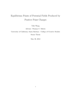
Submitted to SCL on 6 May 2005 On the stable equilibrium points of gradient systems P.-A. Absil∗† K. Kurdyka‡ Abstract This paper studies the relations between the local minima of a cost function f and the stable equilibria of the gradient descent flow of f . In particular, it is shown that, under the assumption that f is real analytic, local minimality is necessary and sufficient for stability. Under the weaker assumption that f is indefinitely continuously differentiable, local minimality is neither necessary nor sufficient for stability. Key words. Gradient flow, Lyapunov stability, cost function, local minimum. AMS subject classifications. 93D05 (Systems theory - Stability Lyapunov), 37N40 (Dynamical systems and ergodic theory - Applications Dynamical systems in optimization and economics), 37B25 ( - Topological dynamics - Lyapunov functions and stability; attractors, repellers), 34D20 (ODE - Stability theory - Lyapunov stability). 1 Introduction Gradient flows are useful in solving various optimization-related problems. Recent examples deal with principal component analysis [YHS01], optimal control [YTM94, JM96], balanced realizations [HM94], ocean sampling [BL02], ∗ School of Computational Science, Florida State University, Tallahassee, FL 323064120, U.S.A. (www.csit.fsu.edu/∼absil). ‡ Laboratoire de Mathematiques (LAMA), Université de Savoie et CNRS UMR 5127, 73-376 Le Bourget-du-Lac cedex, France ([email protected]). † Part of this work was done while the first author was a Research Fellow with the Belgian National Fund for Scientific Research (Aspirant du F.N.R.S.) at the University of Liège. 1 noise reduction [RJ02], pose estimation [BHM94] or the Procrustes problem [TL02]. The underlying idea is that the gradient descent flow will converge to a local minimum of the cost function. It is however well known that this property does not hold in general: the initial condition can e.g. belong to the stable manifold of a saddle point. Not as well known is the fact that, even assuming that the cost function is a C ∞ function, the local minima of the cost function are not necessarily stable equilibria of the gradient-descent system, and vice-versa. The main purpose of this paper is to shed some light on this issue. Specifically, let f be a real, continuously differentiable function on Rn and consider the continuous-time gradient-descent system ẋ(t) = −∇f (x(t)) (1) where ∇f (x) denotes the Euclidean gradient of f at x. Define stability and minimality in the standard way: Definition 1 A point z ∈ Rn is a local minimum of f if there exists > 0 such that f (x) ≥ f (z) for all x such that kx − zk < . If f (x) > f (z) for all x such that 0 < kx − zk < , then z is a strict local minimum of f . An equilibrium point z of (1) is (Lyapunov) stable if, for each > 0, there is δ = δ() > 0 such that kx(0) − zk < δ ⇒ kx(t) − zk < , ∀t ≥ 0. It is asymptotically stable if it is stable and δ can be chosen such that kx(0)k < δ ⇒ lim x(t) = z. t→∞ Then we have: Proposition 2 (i) There exists a function f ∈ C ∞ and a point z ∈ Rn such that z is a local minimum of f and z is not a stable equilibrium point of (1). (ii) There exists a function f ∈ C ∞ and a point z ∈ Rn such that z is not a local minimum of f and z is a stable equilibrium point of (1). The proof given in Section 2 consists in producing functions f that satisfy the required properties. After smoothness, the next stronger condition one may think of imposing on the cost function f is real analyticity (a real function is analytic if it possesses derivatives of all orders and agrees with its Taylor series in the neighborhood of every point). The main result of this paper is that under the analyticity assumption, local minimality becomes a necessary and sufficient condition for stability. 2 Theorem 3 (main result) Let f be real analytic in a neighbourhood of z ∈ Rn . Then z is a stable equilibrium point of (1) if and only if it is a local minimum of f . The proof of this theorem, given in Section 3, relies on an inequality by Lojasiewicz that yields bounds on the length of solution curves of the gradient system (1). Moreover, we give in Section 4 a complete characterization of the relations between (isolated, strict) local minima and (asymptotically) stable equilibria for gradient flows of both C ∞ and analytic cost functions. Final remarks are presented in Section 5. 2 Smooth cost function In this section we prove Proposition 2. Consider f : Rn → R defined by f (x, y) = where g(y) = and h(y) = ( ( 1 g(y)h(y), 1 + x2 e−1/y 0 2 if y 6= 0, if y = 0, y 2 + 1 + sin y12 if y 6= 0, 1 if y = 0. (2) (3) This function is qualitatively illustrated on Figure 1. We show that this function f satisfies the properties of point (i) of Proposition 2 with z = (0, 0). It is routine to check that f ∈ C ∞ , and it is clear that the origin is a local minimum of f , since f is nonnegative and f (0) = 0. The gradient system (1) becomes 2x g(y)h(y) (1 + x2 )2 1 g(y) m(y) ẏ = − 1 + x2 y 3 ẋ = (4a) (4b) where m(y) = 1 + sin y12 − 2 cos y12 + y 2 + 2y 4 . Let (x(t), y(t)) be the solution trajectory of (4) with initial conditions (x(0), y(0)) = (x0 , y0 ) where we pick y0 > 0 and x0 > 0. Then there exists y1 such that 0 < y1 < y0 and m(y1 ) = 2x 2 0. Therefore y(t) > y1 for all t. Then from (4a), ẋ > (1+x 2 )2 g(y1 )y1 whence 3 1 f(x=0,y) 0.8 0.6 0.4 0.2 0 −0.6 −0.4 −0.2 0 y 0.2 0.4 0.6 1 f(x,y=0.4) 0.8 0.6 0.4 0.2 0 −10 −8 −6 −4 −2 0 x 2 4 6 8 10 Figure 1: Plots of f (x, y) along the line x = 0 (above) and y = 0.4 (below). The function f is the one in (2), where g(y) has been replaced by y 2 for clarity of the illustration. lim x(t) = +∞. We have shown that from an initial point arbitrarily close t→+∞ to the origin the solution of (4) escapes to infinity. That is, the origin is not a stable equilibrium point of (4). Point (ii) of Proposition 2 is easier to show. Take f : R → R given by ( g(x) sin x1 if x 6= 0, f (x) = (5) 0 if x = 0 where the function g is given by (3). This function f is illustrated on Figure 2 and straightforwardly verifies the properties in point (ii) of Proposition 2. Notice that both functions f defined in (2) and (5) are nonanalytic at (0, 0). This is not coincidental in view of Theorem 3 which we prove in the next section. 4 0.5 0.4 0.3 f(x) 0.2 0.1 0 −0.1 −0.2 −0.3 −1 −0.8 −0.6 −0.4 −0.2 0 x 0.2 0.4 0.6 0.8 1 Figure 2: Plot of f (x) defined in (5), where g(y) has been replaced by y 2 for clarity of the illustration. 3 Analytic cost function This section is dedicated to proving Theorem 3. We assume throughout, without loss of generality, that f : Rn → R is analytic on an open set U containing the origin, that f (0) = 0 and that ∇f (0) = 0, and we will study the stability of the equilibrium point 0 of the gradient system (1). The proof relies on the following fundamental property of analytic functions. Lemma 4 (Lojasiewicz’s inequality) Let f be a real analytic function on a neighbourhood of z in Rn . Then there are constants c, ρ such that 0 ≤ ρ < 1 and k∇f (x)k ≥ c|f (x) − f (z)|ρ in some neighbourhood of z. Proof. See [Loj65], [BM88], or the short proof in [KP94]. We first prove the “if” part of Theorem 3, i.e., we assume that the origin is a local minimum of f and we show that the origin is a stable equilibrium 5 point (Definition 1) of the gradient system (1). The rationale is based on Lojasiewicz’s argument [Loj84] which provides a bound on the length of the trajectories of (1). Since the origin is a local minimum of f , it follows that there exists a neighbourhood Um of 0 contained in U such that f (x) ≥ 0 for all x ∈ Um . Let x0 be in Um and let x(t) be the solution trajectory of the gradient system (1) with initial condition x(0) = x0 . We shall parameterize x(t) by its arc-length s starting from x0 . By Lojasiewicz’s inequality around the origin, in a neighbourhood UL of the origin k∇f k ≥ c|f |ρ for some ρ < 1 and c > 0. Thus in UL we have on the trajectory x(s) df dx ∇f = h∇f, i = h∇f, − i = −k∇f k ≤ −c|f |ρ . ds ds k∇f k In particular f (x(s)) is decreasing and in Um ∩ UL df 1−ρ ≤ −c(1 − ρ) < 0. ds By integration of this inequality, if x(s) lies in Um ∩ UL for s ∈ [s1 , s2 ] then the length of the segment of curve between s1 and s2 is bounded by c1 (f (x(s1 ))1−ρ − f (x(s2 ))1−ρ ) ≤ c1 (f (x(s1 )))1−ρ where c1 = (c(1 − ρ))−1 . Now let B be a ball of radius > 0 centered on the origin such that B is in Um ∩ UL . By continuity of f , there exists δ < /2 such that f (x) < (/2c1 )1/(1−ρ) for all x ∈ Bδ . If x0 belongs to Bδ then the length of the trajectory x(s) inside B is smaller than c1 (f (x0 ))1−ρ , which is smaller than /2. But since δ < /2 the distance between x0 and the boundary of B is greater than /2. Thus x(t) remains in B for all t, and this is Lyapunov stability. We have proven that minimality is sufficient for stability. The proof of the “only if” part of Theorem 3 uses the following classical convergence result of gradient systems. Lemma 5 Assume that f is a C 2 function and let x(t) be a solution trajectory of the gradient system (1) contained in a compact set K ⊂ Rn . Then x(t) approaches the critical set CK = {y ∈ K : ∇ f (y) = 0} as t approaches infinity, that is, limt→+∞ inf y∈CK ||x(t) − y|| = 0. 6 Proof. The limit points of the trajectories of gradient flows are stationary points [HS74, Thm 9.4.4]. If the solution is bounded then it approaches its positive limit set [Kha96, Lemma 3.1]. We suppose that the origin is not a local minimum of f and we show that the origin is not a stable equilibrium point of the gradient system (1). Since we have assumed that f (0) = 0 and ∇ f (0) = 0, it directly follows from Lojasiewicz’s inequality that there exist an > 0 such that f is zero on the set {y ∈ B̄ : ∇ f (y) = 0}, where B̄ denotes the closed ball of radius centered on the origin. Since the origin is not a local minimum of f , it follows that for all δ > 0, there exists x0 in Bδ with f (x0 ) < f (0) = 0. Then we show that the solution trajectory starting from x0 leaves B̄ and the proof that minimality is necessary for stability will be complete. Suppose for contradiction that the solution trajectory of (1) starting from x0 stays in B̄ for all t. Then, by Lemma 5, x(t) approaches the set {y ∈ B̄ : ∇ f (y) = 0} as t approaches infinity. By continuity of f , it follows that f (x(t)) approaches 0. But f (x(t)) ≤ f (x(0)) < 0 for all t > 0, a contradiction. Note that the “only if” portion of the proof did not make use of Lojasiewicz’s inequality in its full strength. Rather, it only used the following consequence: in some neighbourhood of z, if f (x) 6= f (z) then ∇f (x) 6= 0. This result also follows from the fact that analytic functions admit a finite number of critical values on any compact set. This weaker result will again be sufficient for proving the results discussed in Section 4. 4 Strict minimality and asymptotic stability The previous results were concerned with (simple) Lyapunov stability and (nonstrict) minimality. In this section, we also consider asymptotic stability and strict minimality. A characterization of the relations between Lyapunov stability, asymptotic stability, and various notions of minimality, is displayed in Figure 3; see the caption of the figure for details. In the remainder of this section, we briefly review the relations displayed on Figure 3; see the caption of Figure 3 for the meaning of the initials used below. As before, we assume that f (0) = 0 and ∇f (0) = 0, and we study the stability of the equilibrium point 0 of the gradient system (1). We first consider the case f ∈ C ∞ . LMICP ⇒ ASE follows from Lyapunov’s stability theorem (see [Kha96, Thm. 3.1]). To show ILM ; ASE, R |x| take n = 1 and consider the function f (x) = 0 g(ξ)(1 + sin(1/ξ 2 ))dξ, g as in (3), which exists since the integrand is bounded; any neighbourhood 7 of the origin contains points where ∇ f vanishes, hence the origin is not asymptotically stable1 . SLM ⇒ SE also follows from Lyapunov’s stability theorem (see [Kha96, Thm. 3.1]). LM ; SE is point (i) of Proposition 2. ASE ⇒ LMICP: if the origin is not a LMICP, then either it is not a LM, or it is not an isolated critical point; in both cases, the origin is not an ASE. SE ; LM is point (ii) of Proposition 2. Now we consider the case where f is real analytic. Then, as can be directly shown from Lojasiewicz’s inequality, SLM ⇒ LMICP, and therefore the three properties LMICP, ILM and SLM are equivalent. Since analytic functions are C ∞ , the relations that hold for the C ∞ case remain valid, hence the three properties are also equivalent to ASE. Finally, the relation LM ⇔ SE corresponds to Theorem 3. 5 Final remarks For a general cost function f ∈ C p , p ∈ {2, 3, . . .} ∪ {∞}, the classical way of studying the stability of an equilibrium point (say x = 0) of the gradient descent flow (1) is to consider the Hessian of f at x = 0. If the Hessian is positive definite, then x = 0 is a local minimum and an isolated critical point of f (LCICP in Figure 3); it follows from Figure 3 that the origin is asymptotically stable. But the converse is not true, as the simple example f (x) = x4 shows (the origin is asymptotically stable but the Hessian vanishes). What is more, we have shown that local minima of f are not necessarily stable minima of the gradient system (1), and vice versa. However, the main result of this paper (Theorem 3) ensures that if f is real analytic then the stable points of the gradient descent flow (1) and the local minima of f coincide; the same holds for strict local minima and asymptotically stable equilibria. We refer to Figure 3 for a characterization of the relations between various notions of minimality and stability. This paper is just one step towards understanding the behaviour of gradient flows. Previous advances include: the result by Lojasiewicz [Loj84] that the trajectories of gradient flows cannot have more than one limit point; the proof by Kurdyka et al. [KMP00] of the gradient conjecture of R. Thom stating that the limit of secants exists (see illustration on Figure 4); and the universal bounds for gradient trajectories of polynomial and definable functions given by D’Acunto and Kurdyka [DK04]. 1 Note in this respect that the corollary in section 9.4 of [HS74] is subject to possible misinterpretation: the minimum must be isolated as a critical point to guarantee asymptotic stability. 8 These results, including our Figure 3, remain valid when the Euclidean metric is replaced by a (nondegenerate) Riemannian metric, i.e., when (1) becomes n X Qij (x)∂j f (x) ẋi = − j=1 where Q(x) is a smooth symmetric positive-definite matrix function. Several questions remain open, for instance concerning the existence of lim ẋ/kẋk, the eventual monotonicity of kx(t) − x∞ k, and the case t→+∞ of degenerate Riemannian metrics which has a particular importance for inequality-constrained optimization problems (see, e.g., [AS04]). Finally, note that the relation between minimality and stability for the system ẍ(t) = −∇f (x(t)) —which differs from (1) by the double dot on x(t)— is a classical problem in mechanics. By the Lagrange-Dirichlet theorem, the equilibrium position is stable if the potential f has a strict local minimum at this position. But (nonstrict) minimality is not sufficient for stability [Wie92]. Moreover, the converse of the Lagrange-Dirichlet is not true, but several authors have proposed additional constraints, apart from the absence of a potential minimum, that make the equilibrium unstable; see [RS94] and references therein. Acknowledgements The authors thank A. L. Tits and R. Sepulchre for several useful comments. Part of this work was done while the first author was visiting the second author at the Laboratoire de Mathématiques de l’Université de Savoie. The hospitality of the members of the Laboratory is gratefully acknowledged. References [AS04] P.-A. Absil and R. Sepulchre, Continuous dynamical systems that realize discrete optimization on the hypercube, Systems Control Lett. 52 (2004), no. 3-4, 297–304. MR MR2064925 (2005b:90075) [BHM94] M. Baeg, U. Helmke, and J. B. Moore, Gradient flow techniques for pose estimation of quadratic surfaces, Proc. of the World Congress in Computational Methods and Applied Mathematics, 1994. 9 [BL02] R. Bachmayer and N. E. Leonard, Vehicle networks for gradient descent in a sampled environment, Proc. 41st IEEE Conf. Decision and Control, 2002. [BM88] E. Bierstone and P. D. Milman, Semianalytic and subanalytic sets, Inst. Hautes tudes Sci. Publ. Math 67 (1988), 5–42. [DK04] Didier D’Acunto and Krzysztof Kurdyka, Bounds for gradient trajectories of polynomial and definable functions with applications, submitted, 2004. [HM94] U. Helmke and J. B. Moore, Optimization and dynamical systems, Springer, 1994. [HS74] M. W. Hirsch and S. Smale, Differential equations, dynamical systems, and linear algebra, Academic Press, 1974. [JM96] Danchi Jiang and J. B. Moore, A gradient flow approach to decentralised output feedback optimal control, Systems Control Lett. 27 (1996), no. 4, 223–231. MR 97a:93006 [Kha96] H. K. Khalil, Nonlinear systems, second edition, Prentice Hall, 1996. [KMP00] K. Kurdyka, T. Mostowski, and A. Parusiński, Proof of the gradient conjecture of R. Thom, Ann. of Math. (2) 152 (2000), no. 3, 763–792. [KP94] Krzysztof Kurdyka and Adam Parusiński, w f -stratification of subanalytic functions and the Lojasiewicz inequality, C. R. Acad. Sci. Paris Sér. I Math. 318 (1994), no. 2, 129–133. MR MR1260324 (95d:32012) [Loj65] S. Lojasiewicz, Ensembles semi-analytiques, Inst. Hautes Études Sci., Bures-sur-Yvette, 1965. [Loj84] , Sur les trajectoires du gradient d’une fonction analytique, Seminari di Geometria 1982-1983 (Università di Bologna, Istituto di Geometria, Dipartimento di Matematica), 1984, pp. 115–117. [RJ02] D. Ridout and K. Judd, Convergence properties of gradient descent noise reduction, Physica D 165 (2002), 26–47. 10 [RS94] V. V. Rumyantsev and S. P. Sosnitskiı̆, On the instability of the equilibrium of holonomic conservative systems, J. Appl. Math. Mech. 57 (1994), no. 6, 1101–1122. [TL02] N. T. Trendafilov and R. A. Lippert, The multimode Procrustes problem, Linear Algebra Appl. 349 (2002), 245–264. [Wie92] Z. Wiener, Instability of a non-isolated equilibrium, Arch. Rational Mech. Anal. 116 (1992), no. 4, 301–305. [YHS01] S. Yoshizawa, U. Helmke, and K. Starkov, Convergence analysis for principal component flows, Int. J. Appl. Math. Comput. Sci. 11 (2001), no. 1, 223–236. [YTM94] Wei Yong Yan, Kok L. Teo, and John B. Moore, A gradient flow approach to computing LQ optimal output feedback gains, Optimal Control Appl. Methods 15 (1994), no. 1, 67–75. MR 1 263 418 11 C p, 1 ≤ p ≤ ∞ Real Analytic LMICP LMICP ILM ILM SLM LM ASE SLM SE LM ASE SE Figure 3: Relations between minimality properties of a critical point z of a cost function f and its stability as an equilibrium point of the gradient descent system (1) for f . LM: local minimum; SLM: strict local minimum; ILM: isolated local minimum; LMICP: local minimum and isolated critical point; SE: stable equilibrium; ASE: asymptotically stable equilibrium (see Definition 1 for details). The left-hand graph holds under the assumption that f ∈ C p with p ∈ {1, 2, . . .} ∪ {∞} and the right-hand graph holds for f real analytic. A relation A → B means that property A implies property B, and A 9 B means that property A is not sufficient for property B. All the relations that cannot be deduced by transitivity are 9. 12 x∞ lim x(t)−x0 t→∞ x(t)−x0 x(t) Figure 4: Illustration of the gradient conjecture of R. Thom. 13