COMPUTATIONAL METHODS IN ENGINEERING AND SCIENCE
EPMESC X, Aug. 21-23, 2006, Sanya, Hainan, China
©2006 Tsinghua University Press & Springer
A Stabilized Conforming Integartion Procedure for Galerkin Meshfree
Analysis of Thin Beam and Plate
Dongdong Wang*
Department of Civil Engineering, Xiamen University, Xiamen, 361005 China
Email: [email protected]
Abstract This paper aims to develop an efficient Galerkin meshfree formuation to analyze thin beam and
palte. Through a reformulation of the reproducing conditions (or consistency conditions), an enhanced
meshfree reproducing kernel approximation based on both deflection and slopes is presented. It is shown
that this approximation can approximate a given function with better accuracy than that purely based on the
deflection variables.With this enhanced approximation, the Galerkin meshfree framework for thin beam and
plate is formulated and the integration constraints for bending exactness are derived. Then a refined
stabilized conforming integration is proposed to achieve the exact pure bending solution and remain spatial
stability. Numerical examples demonstrate the present strategy has superior convergence rates, accuracy and
efficiency, compared with that using higher order Gauss qudrature rules.
Key words: meshfree method, thin beam and plate, bending exactness, stabilized conforming intergartion
INTRODUCTION
During the last decade, various kinds of meshfree methods such as SPH, DEM, EFG, RKPM, PUM, H-p clouds, NEM,
MLPG, RPIM, etc., have recerived considerable research attention and have been applied to solve various scientific
and engineering problems [1, 2]. Most of these meshfree methods adopted either the moving least square(MLS) or
reproducing kernel(RK) approximations [1-3]. One remarkable property for the MLS/RK approximation is that global
C 1 conformability can be easily achieved with arbitrary discretizations. This is especially desirable to solve the thin
beam and plate problems which require C 1 approximation under a Galerkin solution process. Krysl and Belytschko
first applied EFG to analyze thin plate problems [4]. Atluri et.al also studied thin beam via MLPG [5]. All these
methods used high order Gauss qudrature to integrate stiffness. As pointed out in [6-8], high order Gauss qudrature
make meshfree methods suffered from lower computational efficiency, and also do not satisfy linear or bending
exactness. To improve computational efficency and as well as reamin spatial stability, in [6] Chen et. al first identified
the linear exactness and corresponding integration constaints and thus proposed the so-called stabilized comfomring
nodal integration (SCNI) for efficient Galerkin meshfree analysis. Later this method was extened to nonlinear
path-independent and path-dependent continuum problems [7]. Wang and Chen futher investigated the bending
exactness and associated integration constaints for shear deformbale paltes, and then developed a locking free plate
formulation based on SCNI [8, 9]. Recently the SCNI methdolody was also successfully adapted to curved beam and
shear deformable shells [10, 11].
In this paper an efficient Galerkin meshfree formuation to analyze thin beam and palte is proposed. First, the
reproducing conditions (or consistency conditions) is reformulated based on based on both the deflection and slopes
which leads to an enhanced meshfree RK approximation accounting the slope influence for the analysis of thin beam
and plate. It is shown that this enhanced approximation can approximate a given function with better accuracy than that
purely based on the deflection variables. Then with this meshfree approximation function, the Galerkin framework for
thin beam and plate is formulated. Since the weak form of thin beam and plate involves the 2nd order derivatives,
accurate numrical integration for the discrete stiffness matrix requires intensive computational effort. In this study,
numerical tests show that low order Gauss quadrature as well as the previous version of stabilized conforming nodal
integration[6-10] which was developed so far to integrate the stiffness with 1st order derivative, can not fully stabilize
⎯ 816 ⎯
the numerical solutions. Correspondingly a refined stabilized conforming integration procedure for thin beam and
plate is proposed. The resulted meshfree scheme still can exactly reproduce bending solutions. Numerical examples
demonstrate the present strategy has superior convergence rates, accuracy and efficiency, compared with that using
higher order Gauss integration rule.
BASIC EQUATIONS
Since thin beam is a one dimensional analogy of thin plate, without lost of generality the proposed formulatations
herein are based on the Kirchhoff thin plate theory.
Figure 1: Sign conventions of a Kirchhoff plate
1. Kinematics and Weak Form
Consider a plate which occupies a domain B = Ω× (−t / 2, t / 2) , where
Ω ⊂ R denotes the mid-plane of the plate with boundary Γ and t is the plate thickness. For convenience of
interpretation the xy plane of a three-dimensional Cartesian coordinate system xyz is set to be coincide with the
middle surface Ω . According to Kirchhoff plate theory, the dependent displacement variable is the transverse
deflection of middle surface: w (x ) . The sign convention adopted in this study is shown in Fig. 1. The rotation and
deformation measures: slope θ (x ) and curvature κ(x ) , thus can be defined as follows:
2
⎧
⎫ ⎧ w ,xx (x ) ⎫
⎪
⎪
⎪ κxx (x ) ⎪⎪⎪ ⎪⎪
⎪
⎪
⎧⎪θx (x )⎫⎪ ⎧⎪w ,x (x )⎫
⎪
⎪
⎪
⎪
⎪
⎪
⎪
⎪
⎪
⎪
⎪
θ (x ) = ⎨
⎬=⎨
⎬ , κ(x ) = ⎨ κyy (x ) ⎬ = ⎨ w ,yy (x ) ⎬
⎪⎪θy (x )⎪⎪ ⎪⎪w ,y (x )⎪
⎪
⎪
⎪
⎪
⎪
⎪ ⎪
⎪
⎪
⎩
⎭ ⎩
⎭
⎪
⎪
⎪2κxy (x )⎪⎭⎪ ⎪⎩⎪2w ,xy (x )⎪⎭
⎩
(1)
The constitutive relation which relates the moment resultant and curvature is:
⎧mxx ⎪⎫
⎡1 ν
⎤
⎪
0
⎪
⎢
⎥
⎪ ⎪⎪⎪
⎪
⎥
m = ⎨myy ⎬ = −Dκ, D = D ⎢ν 1
0
⎢
⎥
⎪⎪ ⎪
⎪
⎢⎢ 0 0 (1 − ν ) / 2⎥⎥
⎪⎩⎪mxy ⎪
⎣
⎦
⎪
⎭
(2)
with D being the flexural rigidity given as D = Et 3 /[12(1 − ν 2 )] . E , ν being the Young’s modulus and Poisson’s
ratio, respectively. The signs of the resultants are consistent with their corresponding kinematic measures as shown in
Fig. 1.
The weak form of a thin plate can be stated as:
∫
Ω
δκT DκdA − δW ext = 0, δW ext = ∫ δwq (x )dA − ∫ h δθn M nnd Γ + ∫ h δwVd Γ
Ω
Γ
Γ
(3)
where q (x ) , M nn and V = Q + M ns ,s = Qx nx + Qyny + M ns ,s are the prescribed distributed transverse pressure,
applied normal moment and quivalent shear force along the natural boundary, respectively. n and s denote the
outward normal and tangential directions of the boundary Γh .
2. Pure Bending A pure bending solution of thin plate has the following form:
w (x ) =
2
∑c
kl
x kyl
k ,l = 0,1, 2
(4)
k +l =0
where ckl ’s are arbitrary constants. To obtain an exact solution in case of pure bending in the numerical solution of the
variational equationof Eq. (3), the meshfree approximation is required to be capable of representing pure bending
⎯ 817 ⎯
modes in Eq. (4), termed Kirchhoff mode reproducing condition (KMRC) in [8]. Later we show that satisfying KMRC
is necessary but not sufficient to achieve a pure bending with Galerkin meshfree formulation. To be bending exact, the
numerical formulation should meet the corresponding integration constraints as well.
MESHFREE DISCRETIZATION & INTEGRATION CONSTRAITS
In this section, the meshfree reproducing kernel (RK) approximation built upon both defelection and rotation variables
is first introduced, and then the necessary conditions for the numerical solution of the weak form to meet bending
exactness are presented.
1. Enhanced RK Approximation Based on Both Defection and Rotations The conventional RK approximation of
displacement field is only based on nodal displacement coefficients. To improve the approximation accuracy, here an
enhanced RK approximation of defection is constructed using both deflection and rotation (derivative of deflection)
variables. Let the plate middle-surface Ω be discretized by a set of NP particles x I , I = 1, 2,..., NP . The RK
approximation of the deflection w (x ) , denoted by w h (x ) , is proposed as follows:
NP
NP
NP
I =1
I =1
I =1
w h (x ) = ∑ ⎢⎣⎡ ΨdI (x )w I + Ψ Iθx (x )θxI + Ψ Iθy (x )θyI ⎥⎦⎤ = ∑ Ψ iI (x )diI ≡ ∑ ΨI (x )dI
(5)
where
ΨI (x ) = {Ψ dI (x ) Ψ Iθx (x ) Ψ Iθy (x )} , dI = {w I
θyI }
T
θxI
(6)
ΨdI , Ψ Iθx and Ψ Iθy are the RK shape functions associated with defection, x -rotation and y -rotation, respectively.
Under the RK framework, they are assumed to take the following forms:
ΨdI (x ) = hT (x I − x )b (x )φa (x I − x ), Ψ Iθx (x ) = hxT (x I − x )b (x )φa (x I − x )
(7)
Ψ Iθy (x ) = hyT (x I − x )b (x )φa (x I − x )
where h , hx and hy are the basis vectors defined as:
h T (x ) = {1, x , y , x 2 , xy , y 2 ,..., x n , ..., y n } , hxT (x ) =
hyT (x ) =
∂h (x )
= {0, 1, 0, 2x , y , 0,..., nx n −1 , ..., 0}
∂x
(8)
∂h (x )
= {0, 0, 1, 0, x , 2y ,..., 0, ..., ny n −1 }
∂y
b (x ) is the unknown coefficient vector to be solved, φa (x I − x ) is a kernel function that supplies smoothness and
locality to the approximation through a compact support measured by ‘a ’. In this study the cubic spline function [1] is
employed, where the 2D kernel function is obtained as a tensor product of two 1D cubic spline functions in x and y
directions.
The coefficient vector b (x ) can be obtained by imposing the following n -th order reproducing conditions:
NP
∑Ψ
I =1
d
I
NP
NP
I =1
I =1
(x )x Ii yIj + ∑ Ψ Iθx (x )(ix I<i −1>yIj ) + ∑ Ψ Iθy (x )(x Ii jyI<j −1> ) = x i y j , i , j = 0, 1, 2,.., n
(9)
where we use the notation: < i > =max {i , 0} .
Eq. (9) can be recast into the following form with shifted basis (x I − x ) :
⎡ ΨdI (x )(x I − x )i (yI − y ) j + Ψ Iθx (x )i (x I − x )<i −1> (yI − y ) j ⎤
⎢
⎥ = δ δ , i , j = 0,1, 2..., n
∑
i0 j0
θy
i
< j −1>
⎢
⎥
I =1 ⎣⎢+Ψ I (x )(x I − x ) j (y I − y )
⎦⎥
NP
(10)
or in a matrix form as:
NP
∑ ⎣⎢⎡ Ψ
I =1
d
I
(x )h (x I - x ) + Ψ Iθx (x )hx (x I - x ) + Ψ Iθy (x )hy (x I - x )⎦⎥⎤ = h (0 )
Substituting Eq.(7) into Eq.(11) gives
⎯ 818 ⎯
(11)
M(x )b (x ) = h (0)
(12)
with M being the moment matrix given by
⎡h (x I − x )h T (x I − x )φa (x I − x ) + hx (x I − x )hxT (x I − x )φa (x I − x )⎤
⎥
M(x ) ≡ ∑ ⎢⎢
⎥
T
⎥
I =1 ⎢+hy (x I − x )h x (x I − x )φa (x I − x )
⎣
⎦
NP
(a)
(13)
(b)
(c)
Figure 2: Enhanced RK shape functions: (a) Ψ dI ; (b) Ψ Iθx ; (c) Ψ Iθy
Thus we obtain b (x ) = M−1 (x )h (0) , and the meshfree shape functions are finally obtained as
ΨdI (x ) = hT (x I )M−1 (x )h (x )φa (x I − x ), Ψ Iθx (x ) = h T (x I )M−1 (x )hx (x )φa (x I − x )
Ψ Iθy (x ) = hT (x I )M−1 (x )hy (x )φa (x I − x )
(14)
Fig. 2 shows the shape functions of Eq. (14). The comparisons between the current RK approximation with slope
enhancement (RKSE) and the original RK approximation only using nodal deflections are shown in Fig. 3, where the
interpolation errors of a function f (x ) = x 4 , x ∈ [−10,10] are compared. It can been the enhanced RK approximation
yields better accuracy. In this paper the error norms are defined as follows:
L2 error = ⎢⎡ ∫ ( f − f h )2 dx ⎥⎤
⎣ Ω
⎦
1/ 2
; H s 1 error = ⎢⎡ ∫ ( f,x − f,xh )2 dx ⎥⎤
⎣ Ω
⎦
1/ 2
; H s 2 error = ⎢⎡ ∫ ( f,xx − f,xxh )2 dx ⎥⎤
⎣ Ω
⎦
(a)
1/ 2
(15)
(b)
Figure 3: Comparisons of interpolation errors for f (x ) = x 4 : (a) L2 error; (a) H s 1 error
In [5], a generalized moving least squares approximation which also accounts the rotations was proposed and used for
thin beam analysis. Note in Eq. (14) the shape function employs shifted basis functions h (x I − x ) , hx (x I − x ) ,
hy (x I − x ) which turns out to give the moment matrix a better conditioning number.
2. Kirchhoff Mode Reproducing Condition (KMRC) Using the RK shape functions of Eq. (14), the rotation and
curvature are approximated as:
⎯ 819 ⎯
⎧⎪ κxxh (x ) ⎫⎪
⎪⎪
⎪⎪ NP
⎧θxh (x )⎪⎫ NP
⎪
h
h
θ h (x ) = ⎪
⎨ h ⎪⎬ = ∑ AI dI , κ (x ) = ⎪⎨ κyy (x ) ⎪⎬ = ∑ BI dI
⎪⎪θy (x )⎪⎪ I =1
⎪⎪ h
⎪ I =1
⎩
⎭
⎪⎪⎩2κxy (x )⎪⎪⎪⎭
(16)
where
⎡ Ψd
AI = ⎢⎢ dI ,x
⎣⎢ Ψ I ,y
Ψ
Ψ
θx
I ,x
θx
I ,y
Ψ
Ψ
θy
I ,x
θx
I ,y
⎡ ΨdI ,xx
⎢
⎤
⎥ , B (x ) = ⎢ Ψd
I
⎢ I ,yy
⎥
⎢2 Ψd
⎦⎥
⎣⎢ I ,xy
Ψ Iθx,xx
Ψ Iθx,yy
2Ψ Iθx,xy
Ψ Iθy,xx ⎤⎥
Ψ Iθy,yy ⎥⎥
2 Ψ Iθy,xy ⎥⎦⎥
(17)
Let dIb denote the coefficient vector of a pure bending deformation according to Eq. (4):
2
⎧⎪
⎫
⎪⎪ ∑ c x k y l ⎪⎪⎪
kl I I
⎪⎪ k +l =0
⎪⎪
⎪⎪
⎪⎪
⎪⎪ 2
b
<k −1> l ⎪
dI = ⎨ ∑ ckl kx I
yI ⎪⎬
⎪⎪k +l =0
⎪⎪
⎪⎪ 2
⎪⎪
⎪⎪
k <l −1> ⎪
⎪⎪
⎪⎪ ∑ ckl x I lyI
⎪⎭⎪
⎩⎪ k +l =0
(18)
The reproduction of the pure bending mode in the RK approximation implies:
∑B d
I
b
I
= const.
(19)
I
Substituting Eq. (18) into Eq. (19) yields:
NP
∑ ⎣⎢⎡ Ψ
d
I ,αβ
I =1
(x Ik yIl ) + Ψ Iθx,αβ (kx I<k −1>yIl ) + Ψ Iθy,αβ (x Ik lyI<l −1> )⎤⎦⎥ = (x k y l ),αβ , k + l = 0, 1, 2
(20)
where the subscripts α, β represent the partial differentiation with respect to x , y respectively.
It is straightforward to show that based on the reproducing properties of Eq. (9), the above conditions of Eq. (20) can
be satisfied by selecting the following 2nd (or higher) order basis functions in the RK approximation:
h T (x ) = {1, x , y , x 2 , xy , y 2 }
(21)
3. Integration Constraints for Bending Exactness To pass pure bending test under Galerkin framework, the quadratic basis
functions of Eq. (21) should be employed in the RK approximation, and moreover we need to investigate the integration
requirement for the domain integration of the weak form. The integration constraints are identified by enforcing the pure bending
mode to satisfy the discrete equilibrium equation. In case of pure bening, it is convenient to express the external virtual work by
the applied moments as:
δW
ext
⎡nx
⎪⎧M b ⎪⎫
T
= −∫ h δθ h M bd Γ, M b = ⎪⎨ xb ⎪⎬ = Nm b , N = ⎢
⎢0
Γ
⎪
⎪
⎪
⎣
⎩M y ⎪
⎭
0
ny
ny ⎤
⎥
nx ⎥⎦
(22)
Thus the weak from of Eq.(3) becomes:
∫
Ω
T
T
δκh Dκhd Ω = − ∫ h δθ h M bd Γ
(23)
Γ
The resulting discrete equation is
∫
Ω
BIT DBd bd Ω = −∫ h AIT M bd Γ
(24)
Γ
Based on Eq. (19) , it is seen that m b = −DBd b = const. , and thus we have
∫
Ω
BIT d Ωm b = ∫ h ΕIT d Γm b
(25)
Γ
and
⎯ 820 ⎯
⎡ ΨdI ,x nx
⎢
T
T
T
T
⎢ Ψ θx n
Ω
=
Γ
=
=
B
Ε
,
Ε
A
N
d
d
I
I
∫Ω I
∫Γh I
⎢ I ,x x
⎢ Ψ θy n
⎢⎣ I ,x y
ΨdI ,y ny
Ψ Iθx,y ny
Ψ Iθx,y ny
ΨdI ,x ny + ΨdI ,y nx ⎤⎥
Ψ Iθx,x ny + Ψ Iθx,y nx ⎥⎥
Ψ Iθy,x ny + Ψ Iθx,y nx ⎥⎥⎦
(26)
Eq. (26) is the integration constraint the numerical scheme for thin plate needs to meet. After using the numerical
domain integration the discrete counterparts of Eq. (26) are
N int
∑B
I
(x i )ωi = 0 for nodes {I
supp(Ψ I ) ∩ Γh =∅}
i =1
N int
∑B
J
i =1
(27)
NBint
(x i )ωi = ∑ ΕJ (x j )ω j for nodes
{J
supp(ΨJ ) ∩ Γ ≠ ∅}
h
j =1
where N int and NBint are the total number of integration points for domain and boundary integrations, respectively;
x i and x j are the nodal and the boundary sampling points, and ωi and ω j are their corresponding integration
weights.
METHOD OF REFINED STABILIZED CONFORMING INTEGRATION
1. Refined Curvature Smoothing To meet the integration constraints of Eq. (27) and remain stability, a refined
stabilized conforming integration procedure for thin beam and plate is developed here. The basis for the stabilized
conforming integration is the strain or curvature smoothing for plate. A natural extension of our previous work [6-9]
would be introducing the following curvature smoothing at a given nodal point x K :
κ%αβ (x K ) =
1
AK
∫
ΩK
καβ (x )d Ω =
1
2AK
∫
(w ,αβ + w ,βα )d Ω =
ΩK
1
2AK
∫
ΩK
(w ,αn β + w ,β nα )d Ω
(28)
where AK is the area of nodal representative domain ΩK , and the divergence theorem has been invoked. Now if we
introduce the RK approximation into (28) we get similar expressions for the smoothed nodal gradient as in [8].
However, our numerical tests show that low order Gauss quadrature as well as this direct extension of previous SCNI
[6-9] which was developed to integrate the stiffness with 1st order derivative, can not fully stabilize the numerical
solutions for the thin beam and plate where the 2nd order derivative occurs in the weak form.
To obtain the pure bending solution and remain spatial stability as well, the curvature smoothing idea in the stabilized
conforming nodal integration is extended here. Rather than diectly employing the nodal strain smoothing as Eq. (28),
the representative domain ΩK is further partitioned into IK sub-domains ΩKi as hown in Fig. 4 , and the nodal
curvature smoothing is carried out as follows:
κ%αβ (x K ) =
1
AK
∫
ΩK
καβ (x )d Ω =
1
AK
IK
∑∫
i =1
ΩKi
καβ (x )d Ω =
1
2AK
IK
∑∫
i =1
ΓKi
(w ,αn β + w ,β nα )d Γ
Figure 4: Nodal representation domain for curvature smoothing
Introducing the enhanced RK approximation into (29) gives
⎯ 821 ⎯
(29)
NP
κ% h (x K ) ≡ ∑ B% I (x K )dI
I =1
% 1
% 2
% 3
⎡∇
⎤
⎢ 1 Ψ I ,1 (x K ) ∇1 Ψ I ,1 (x K ) ∇1 Ψ I ,1 (x K ) ⎥
% Ψ1 (x ) ∇
% Ψ 2 (x ) ∇
% Ψ 3 (x ) ⎥ , ∇
% Ψ j (x ) = 1
B% I (x K ) = ⎢⎢ ∇
β I ,α
2 I ,2
2 I ,2
2 I ,2
K
K
K ⎥
K
AK
⎢2∇
% Ψ 1 (x ) 2∇
% Ψ 2 (x ) 2∇
% Ψ 3 (x )⎥
2 I ,1
2 I ,1
K
K ⎥⎦
⎢⎣ 2 I ,1 K
(30)
IK
∑∫
i =1
ΓKi
j
I ,α
Ψ n βd Γ
2. Discrete Equations Introducing the smoothed curvature of Eq. (30) and the enhanced RK approximation of Eq. (5)
into the nodally integrated weak form with an assumed strain method yields the following discrete variational
equation:
NP
∑ [δκ%
hT
K =1
NP
NBint
K =1
L =1
(x K )Dκ% h (x K )]AK = ∑ [δw h (x K )q (x K )]AK + ∑ ⎡⎢⎣δw h (x L )V (x L ) − δθnh (x L )M nn (x L )⎤⎥⎦ ωL
(31)
and then the meshfree discrete equation becomes:
NP
Kd = f , K IJ = ∑ B% IT (x K )DB% J (x K )AK
K =1
NP
NBint
(32)
fI = ∑ Ψ (x K )q (x K )AK + ∑ ⎢⎣⎡Ψ (x L )V (x L ) − A (x L )n (x L )M nn (x L )⎤⎥⎦ ωL
T
I
K =1
T
I
T
I
L =1
Due to the conforming nature of sub-domains used for curvature smoothing, following the derivation in [6-8], it is
pretty straightforward to show that the above Galerkin meshfree scheme exactly satisfies the integration constraints of
Eq. (27) and thus can reproduce bending solutions with the basis of Eq. (21). Our numerical experiments show that
since now the stiffness involves the 2nd order derivatives which have more complex shapes than the 1st order
derivatives, to get a reasonable solution accuracy 6-point or higher Gauss qudrature is required for thin beam, or 6 × 6
qudrature rule for thin plate. On the other hand, using the proposed method for curvature smoothing two sub-domains
in 1D or four subdomains in 2D already give execellent slution accuracy and superior convergence rates. It turns out
the proposed approach is quite robust and cost effective.
NUMERICAL TESTS
1. Pure Bending of Clamped-Free Beam
Figure 5: A clamped-free beam under pure bending
(a)
(b)
Figure 6: Solution errors of calmped-free beam subjected to pure bending: (a) Deflection; (b) Curvature
The geometry and material properties of the beam as shown in Fig. 5 are: L = 10 , cross section width b = 1 and height
t = 1 , Young’s modulus E = 2 ×10⁶ , The beam is subjected to a moment M = 1000 at the end. In the numerical test,
⎯ 822 ⎯
a 11 point uniform discretization is used. The errors of numerical solutions via different integration schemes are
compared in Fig 6(a)-(b), where SCI-2 denotes the proposed method with 2 subdomains equally divided in each nodal
reprenstative domain, GI-3 and GI-6 represent the Gauss integration with 3-point and 5-point quadrature rules,
respectively. Here the errors are normalized by the exact tip solutions. The quadratic basis is employed throught this
study and the normalized support size of kernel function in the enhanced RK approximation is set to be 3 . The
numerical results for pure bending in The results show that the proposed SCI approach can exactly reproduce the
bending mode. On the other hand GI-3 gives less accurate unstable solutions and even GI-6 yields considerable errors.
For this example our tests also show that the solutions blow up using either GI-2 or SCI-1 (previous version of
stabilized conforming nodal integration). Moreover, we would like point out that since the proposed SCI meets the
derived integration constraints, it can produce the exact solutions regardless of the discretization pattern.
2. Clamped-Free Beam under Uniform Loading
Figure 7: A clamped-free beam under pure bending
(a)
(b)
(c)
(d)
Figure 8: Solution error comparisions of calmped-free beam subjected to uniform bending:
(a) Dflection; (b) Rotation; (c) Curvature; (d) CPU time
As shown in Fig. 7, the clamped-free beam is under uniform load q=100. The geometry and material properties are the
same as previous example. The quadratic basis and kernel function with normalized support size of 3 again are used
herein. Figure 8(a)-(d) lists the convergence rates comparisons of different error norms and CPU time cost by various
solution methodologies. The results clearly show the proposed SCI method gives superior convergence behavior with
much less CPU cost compared to those using GI. It is noted that even SCI-2 yields better solution accuracy than GI-6 or
GI-8 (8-point Gauss integration) as refinement grows. So it is reasonable to use SCI-2 in consideration of both accuracy
and efficiency. On the other hand, the CPU cost of SCI strategy is much lower (5 or 6 times faster), as can be seen from
⎯ 823 ⎯
Fig. 6(d), even SCI-3 (SCI using 3 subdomains in each nodal reprenstative domain) is more efficient than GI-3. The
reason behind this is that SCI totally avoids the computation of 2nd order derivative of shape function which for
meshfree methods is very time consuming, i.e, 1st order derivative is a sum of three terms while after differentiation the
2nd order derivative becomes a nine term summation and thus computational effort is increased intensively.
CONCUSIONS AND FUTURE WORK
A stabilized conforming integration approach has been proposed for Galerkin meshfree analysis of thin beam and plate
based on an ehanced RK approximation. This enhanced RK approximation was constructed using both the deflection
and nodal roations as the nodal variables. To achive bending exactness under Galerkin meshfree framework, the
corresponding requirements for RK approximation and integration constraints were derived. Then a refined nodal
curvature smoothing approached was proposed to meet the integration constraints as well as to stabilize the dicretized
weak form. In this method, the nodal representative domain is further divided into several sub-domains and the nodal
curvature smoothing is obtained as a summation of contributions form all sub-domains. The smoothing and
conforming nature ensures the proposed approach can exactly satisfy the integration constraints. Numerical bending
tests of thin beam have showed that the proposed approach exactly reproduces pure bending mode for arbitrary
discretization. In this case it has also been observed the relatively lower order Gauss quadrature GI-3 yields less
accurate solutions and even higher order Gauss quadrature GI-6 produces considerable errors. The convergence tests
have demonstrated the the proposed SCI approach gives superior convergence rates over those of GI with a much
lower CPU cost. Both accuracy and efficiency are achieved in the present formulation. Numerical tests for various
benchmark plate problems will be studied next to further validate the proposed method.
Acknowledgements
The support of this work by the Scientific Research Foundation for the Returned Overseas Chinese Scholars, State
Education Ministry of China and the Research Initiation Fund of Xiamen University is gratefully acknowledged.
REFERENCES
1.
Belytschko T, Krongauz Y, Organ D, Fleming M, Krysl P. Meshless methods: an overview and recent
developments, Comput. Meth. Appl. Mech. Eng., 1996; 139: 3-47.
2.
Li S, Liu WK. Meshfree particle methods, Springer-Verlag, 2004.
3.
Liu WK, Jun S, Zhang YF. Reproducing kernel particle methods, Int. J. Numer. Meth. Fluids, 1995; 20:
1081–1106.
4. Krysl P, Belytschko T. Analysis of thin plates by the element-free Galerkin method. Comp. Mech., 1995; 16:
1-10.
5. Atluri S.N, Cho JY, Kim HG, Analysis of thin beams, using the meshless local Petrov-Galerkin method, with
generalized moving least squares interpolations. Comp. Mech., 1999; 24: 334-347.
6. Chen JS, Wu CT, Yoon S, You Y. A stabilized conforming nodal integration for Galerkin meshfree methods. Int.
J. Numer. Meth. Eng., 2001; 50: 435-466.
7. Chen JS, Yoon S, Wu CT. Nonlinear version of stabilized conforming nodal integration for Galerkin meshfree
methods, Int. J. Numer. Meth. Eng., 2002; 53: 2587-2615.
8. Wang D, Chen JS. Locking-free stabilized conforming nodal integration for meshfree Mindlin-Reissner plate
formulation. Comput. Meth. Appl. Mech. Eng., 2004; 193: 1065-1083.
9. Wang D, Dong SB, Chen JS. Extended meshfree analysis of transverse and inplane loading of a laminated
anisotropic plate of general planform geometry. Int. J. Solids Struct., 2006; 43: 144-171.
10. Wang D, Chen JS. Constrained reproducing kernel formulation for shear deformable shells, Proceeding of the 6th
World Congress on Computational Mechanics, Beijing, September 5-10, 2004.
11. Wang D, Chen JS. A locking-free meshfree curved beam formulation with the stabilized conforming nodal
integration. Comp. Mech., 2006; in press (DOI 10.1007/s00466-005-0010-0).
⎯ 824 ⎯
© Copyright 2026 Paperzz