I
..I
I
I
I
I
I
I
BRANCHING PROCESSES IN STOCHASTIC ENVIRONMENTS
by
William E. Wilkinson
University of North Carolina
Institute of Statistics Mimeo Series No. 544
September 1967
I
Ie
I
I
I
This research was supported by the Department of the
Navy, Office of Naval Research. Grant NONR-855(09).
I·
I
'.
I
I
DEPARTMENT OF STATISTICS
University of North Carolina
..
Chapel Hill, N. C•
~
...•.l
I
'.I
I
I
I
I
I
I
I
ii
TABLE OF CONTENTS
Chapter
ACKNOWLEDGEMENTS
,
I.
I
I
iii
ABS'rRACT
I
II
Ie
I
I
I
I
Page
INTRODUCTION AND PRELIMINARY RESULTS
1.
Introduction and description of the process
1
2.
The generating function and moments of Z
4
3.
Instability of Z
5
4.
Martingales
IV
n
n
and convergence of IT
n
7
CONDITIONS FOR ALMOST CERTAIN EXTINCTION
5.
Introduction
10
6.
The dual process
12
7.
Some special cases
13
8.
The Lindley process
20
9.
Conditions for almost certain extinction
24
Comparison with related processes
31
10.
III
iv
EXTINCTION PROBABILITIES
11.
Introduction
39
12.
Moments of the dual process
39
13.
Equations for extinction probabilities
42
14.
The case of two environmental states
48
MARKOV ENVIRONMENT
15.
Description of the process
60
16.
First and second moments of Z
--n
63
17.
The generating function of population size at epochs
64
18.
Extinction probabilities
66
BIBLIOGRAPHY
71
I
iii
'.I
I
I
I
I
I
I
I
ACKNOWLEDGEMENTS
It is a pleasure to acknowledge indebtedness to Professor
Walter L. Smith for suggesting this problem, for providing invaluable
guidance, and for his patience during the long period at the outset of
this investigation when results seemed at hand, but yet, were
unobtainable.
Above all, however, I value having had the privilege of
working with him.
Professor M. R. Leadbetter has been a source of encouragement
throughout, and has made a number of suggestions for improving the
final manuscript.
Professor A. C. Mewborn gave freely of his time on
several occasions to discuss aspects of matrix theory which arose in
the course of the investigation.
Mrs. Bobbie Wallick typed the final manuscript quickly and with
Ie
special attention to its overall appearance.
I
I
I
I
provided by the Woodrow Wilson Foundation, the Office of Naval Research,
I
I.
t
I
Financial assistance for my graduate study and research has been
and the Department of Statistics, and is gratefully acknowledged.
To my wife, Frankie, for her sustained confidence and encouragement, go my most heartfelt thanks.
I
I.
"I
I
I
I
I
I
I
Ie
iv
ABSTRACT
This paper is concerned with two simple models for branching processes in stochastic environments.
The models are identical to the
model for the classical Galton-Watson branching process in all respects
but one.
In the family-tree language commonly used to describe branch-
ing processes, that difference is that the probability distribution for
the number of offspring of an object changes stochastically from one
generation to the next, and is the same for all members of the same
generation.
That is, the probability distribution of the number of off-
spring is a function of the "environment."
The two models considered
herein have a random environment and a Markov environment.
In the
classical Galton-Watson process, it is assumed that the families of distinct objects in a given generation develop independently of one another.
This independence, which renders the Galton-Watson process so tractable
mathematically, is lacking in the stochastic environment models.
The
I
object of study is the probability distribution of the number of objects
I
I
of conditions under which the family has probability one of dying out.
I
I
'.
t
I
Zn in the nth generation.
Of particular interest is the determination
In the random environment model, the asymptotic behavior of the probability generating function for Z
n
(and, consequently, the question of
extinction probability) is studied by analyzing the asymptotic behavior
of a closely related Markov process on the unit interval.
Necessary and
sufficient conditions for extinction with probability one are obtained
in the case of a finite number of environmental states; for a denumerably
infinite number of environmental states, an additional condition, which
has not been shown to be necessary, is required, and this precludes
v
obtaining necessary and sufficient conditions fot' almost certain extinction.
In some special cases, procedures are given for approximating
extinction probabilities when the population has a non-zero chance of
survjving indefinitely.
The asymptotic behavior of the probability
generating function for family size in the Markov environment model is
studied by relating it to a probability generating function of the type
obtained in the random environment model.
I
.'I
I
I
I
I
I
I
I
_I
I
,
I
I
,
.'I
I
I
I.
I
I
I
I
I
I
I
I
Ie
I
I
I
I
I
I
.I
CHAPTER I
INTRODUCTION AND PRELIMINARY RESULTS
1.
Introduction and description of the process
In the preface to The Theory of Branching Processes, Harris (1963)
defines a branching process as "a mathematical representation of the
development of a population whose members reproduce and die, according
to laws of chance.
The objects may be of different types, depending on
their age, energy, position, or other factors.
interfere with one another."
However, they must not
This assumption, that different objects
reproduce independently, unifies the mathematical theory and characterizes virtually all of the branching process models in the literature.
While this assumption allows the definition to encompass a large number
of models, it also limits the application of the models of branching
processes, since the natural processes of multiplication are often
affected by interactior among objects or other factors which introduce
dependencies.
,
The model with wHich we shall be concerned in the first three
chapters may be described mathematically as follows.
Let {p } be a
r
finite or denumerablyinfinite sequence of nonnegative real numbers
satisfying
~
r
p
r
= 1, and let
{~
r
(s)} be a corresponding sequence of
probability generating functions.
PO:1
j
= coeffiqient of sj in
,.
Define a matrix (P
ij
) with elements
r~ p r [~ r (s)]\lsl -< 1,
i,j = 0,1,· ...
(1.1)
2
Clearly P
> 0 for all i and j, and since
ij
(1.2)
it follows that
J Pij
=I
for all i.
We can define a temporally homogeneous Markov chain {Z } on the
n
nonnegative integers by choosing initial probabilities
P{Zo
for some positive integer
= i) =
I, i
tS
i,K - { 0, i ., K
K,
P{Zo = a 0' ••• ,
= i)
> 0, then P
ij
.'I
I
I
I
=K
-
and defining
If P{Zn
I
is the transition probability
p{Zn +1 = jlZn = i).
While all our results follow from the mathematical description of
the model given above, we may interpret the process {Z } as a branching
I
I
I
I
_I
n
process
I
developing in an environment which changes stochastically in
time and which affects the reproductive behavior of the population.
For example, the development of an animal population is often affected
by such environmental factors as weather conditions, food supply, and
so forth.
In the physical interpretation of the model considered in
the first three chapters, what we have in mind is that the environmen-
I
t
I
,
tal factors which affect reproductive behavior can be classified into
a countable number of "states," and that these states of the environment
~e shall refer to the stochastic process {Zn } as a branching
process, even though the objects rep~oduce independently only in a
conditional sense.
I'
.1
I
I
I
I.
I
I
I
I
I
I
I
I
Ie
I
I
I
I
I
I.
I
I
3
are sampled randomly from one generation to the next.
As in the classical Galton-Watson process [cf. Harris (1963),
Chapter I], we consider objects that can generate additional objects of
the same kind.
The initial set of objects, called the zeroth generation,
has offspring that constitute the first generation; their offspring
constitute the second generation, and so on.
Since we are interested
only in the sizes of the successive generations, and not the number of
offspring of individual objects, we shall let Z , n
n
= 0,1,···, denote
the size of the nth generation, and shall always assume that Zo = 1,
unless stated otherwise.
In the Galton-Watson process, it is assumed that the number of
offspring of different objects are independent, identically distributed
random variables with probability generating function
our model, the probability generating function
~(s)
~(s),
If
= 1,2,···,
~ r (s)
=
.E
In
is replaced by one
~
of a countable number of probability generating functions
r
say.
r
(s),
depending on the "state" of the environment at the time.
J=l
p jsj,then p j is interpreted as the probability that
r
r
an object existing in the nth generation and environmental state r has
j offspring in the
(n+1)~
generation.
That is, we assume that the environment passes through a sequence
of states governed by a process {V } of independent, identically disn
tributed random variables with
n = 0 1 •..
'"
independent of n.
r = 1 2 ..•. L P
'"
r
= 1
'
Then, given that V = r, the number of offspring of
n
different objects in the nth generation are independent, identically
distributed random variables with probability generating function
~
r
(s).
4
Without loss of generality, we shall assume that p
We shall further assume throughout that, unless
~tated
r
>
0 for all r.
otherwise, the
following basic assumptions are satisfied:
(but Vo is random);
a)
Zo = 1
b)
m = ep' (1) is finite for all r;
r
r
c)
Pro < 1 for all r, and pro + Prl < 1 for some r (.1.£,. at least
one ep (s) is strictly convex on the unit interval).
r
2.
The generating function and moments of Zn
Let TIn(s) designate the probability generating function of Zn'
n
= 0,1,···.
Theorem 2.1
The generating function of Zn is given by
n
wher~consistent with
= 1,2,···,
Assumption (a), TIO(s) = s.
Proof.
TI (s) = E(sZu)
n
Z
00
= i)E(s nlz
= i)
= i~O P(Z
n-l
n-l
=
from (1.2).
00
E P(Z
= i){E P [ep (s)]:L}
n-l
r r r
i=O
Rearranging the double series, we obtain
TI (s)
n
= Er p r {iEO
=
P(Z
n-l
= i)[ep r (s)]i}
(2.1)
I
.1
I
I
I
I
I
I
I
I
_,
I
I
I
I
I
and the proof is complete.
By repeated application of (2.1), we obtain the representation
.-I
I
I
5
I.
I
I
I
I
I
I
I
I
Ie
I
I
I
I
I
I.
I
I
(2.2)
which we will use in Chapter II.
2
Let m = EZ l (= L pm) and y = I: pm.
r r r
r r r
If m
<
00,
we can differen-
tiate (2.1) at s - 1 and obtain
II'(l) = L P II' (1)4>'(1)
n
r r n-l
r
mIl'
n-l
(1),
n
so by induction, II~(l) = m , n = 0,1,···.
If II 1(1)
<
00,
we can
differentiate (2.1) again, obtaining
II" (1)
L P
r
n
= yll"
r
{II" (1)[<1>'(1)]2 + II' (1)4>"(1)}
n-l
r
n-l
r
n-l
(1)
+ II '1' (l)mn -
l •
We thus obtain
n-l
L i n-l-i
II" (1) = II"(l)
1
i=O Y m
n
n
= 1,2,'"
and
Var Zn -_ II'l'(l)
n-l.
.
~
1
n-1-1
i~O y m
+ mn(l - mn) ,
n =
1,2,···.
(2.3)
Hence we have the following result.
Theorem 2.2.
00.
If EZ 1 <
Var Z
Ii
3.
n
00.
then EZ n_=--'m""-........_n_ _=_0..;;..L.1~._._._....._a;;;;;n;;;;,d",-1;;;.·f;;;.
is given by (2.3).
Instability of Zn and convergence of lIn
The state space of the Markov chain Z , n = 0,1"", is the set S
n
of nonnegative integers.
P (Z
n+t
=
Z
The state
ZES
is said to be transient if
for some t = 1 2 •••
"
Izn
= z) < 1.
6
Theorem 3.1
If z is a positive integer. then
P(Zn+t
=z
for some t
= 1,2,···lzn = z)
<
(3.1)
1.
It follows that for an arbitrary positive integer N,
P(O
Proof.
If
~
r
as n
< N) ~ 0
< Z
n
~
00.
(0) > 0 for some r, then
P(Z
= olzn =
n+1
O.
z) >
Hence
=z
P(Zn+t
for some t
= 1,2,···lzn = z)
< 1 -
P(Z
= olzn = z)
n+1
<
1,
<
1,
so the state z is transient.
If
~
r
(0)
=0
for all r, then since at least one
~
is strictly
r
convex,
P(Zn+1
But
~
r
=0
(0)
P(Zn+t
=z
>
zlzn
= z)
>
O.
for all r implies that Z is nondecreasing, so that
n
for some t
= 1,2,···lzn = z)
<
-
1 - P(Z
n+1
>
zlz
n
= z)
and the proof of (3.1) is complete.
If i is a positive integer, we have just shown that the state i is
transient.
It follows [Feller (1957), p. 353] that
lim P(Zn
n~
= i) = O.
Hence
P(O
Theorem 3.2
< Z
n
< N) ~ 0
as n
For sE[O.l),
lim IT n (s) = c
n~
<
1.
~
00.
I
-'I
I
I
I
I
I
I
I
_I
I
I
I
I
I
I
-.
I
I
II
I
I
I
I
I
I
I
Ie
I
I
I
I
I
I
II
7
Proof.
IT (0) is a nondecreasing function of n, and so tends to a limit
n
c, say (0 < c
~
1), as n tends to infinity.
If N is a positive integer,
N
•
IT (s) = P(Z = 0) + 1.'-~1 P(Zn = i)s
n
n
1.
00
Given s, 0 < s < 1, and an arbitrarily small
large that sN+l/(l - s)
<
E/2.
r
E >
0, choose N sufficiently
Then
p(Z
i=N+l
•
1.
+ i=N+l
L P(Zn = i)s •
n
= i)si
E/2.
<
By the latter half of Theorem 3.1, we can choose n sufficiently large
that
i) < E/2.
Thus for n sufficiently large,
IT (s) < IT (0) +
n
n
E,
that is,
lim IT (s) < c +
n
Since
E
-
E.
is arbitrary, we have lim IT (s) < c.
n
-
But IT (0)
n
<
IT (s),
n
so c < lim IT (s), and the proof is complete.
--
4.
n
Martingales
In this section, we shall assume that m = L m is finite.
r
~
n
n
= Zn 1m,
n
r
= 0,1,···.
From the definition of Z , we have with probability one,
n
E(Zn+lIZn) = mZ ,
n
n = 0,1, .. ••
Hence, with probability one,
Let
8
I
.1
k
····=mZ,
k,n
n
= O,l,···.
Dividing both sides by mn+k , we obtain
the first equality holding because
~O' ~1'···
~O' ~1'···
second equality in (4.1) reveals that
Since
E~
n
= 1,
~
Markov chain.
The
is a martingale.
n· 0,1,···, it follows from a theorem of Doob
(1953, Theorem 4.1, p. 319) that n-kXl
lim
and
is
~
n
..
~
exists with probability one,
L
E~ <
In the very special case where m . is independent of r (m
r
r
= m),
we
can obtain a stronger result.
Theorem 4.1
If mr
v~riables ~n
converge with probability one and in mean square to a
random variable
~
=
m for all r. m > 1 and EZf < ..;. then the random
Proof.
~ =
1, Var
Var Zl / (m2 - m).
By the same theorem of Doob, we have only tQ prove that
lim E~2
n+oo
n
<
00
to obtain mean square convergence.
E~2
n
= m- 2n
n"(l)
But Y = ~ Prm~ .. m2 , and nr(l)
E~~
=
_I
with
~ =
1
n-1
I:
i=O
= Var
From (2.3),
yimn-1-i + m-n •
Zl + m(m - 1), so we have
n-1
[Var Zl + m(m - 1)]m-2n i~O m2i+n-1-i + m-n
.. [Var Zl + m(m - 1)]m-(n+1) (mn - l)/(m - 1) + m-n
Var Zl
-n
_ 1) (1 - m ) + 1 •
= m(m
I
I
I
I
I
I
I
I
(4.2)
I
I
I
I
I
I
-.
I
I
II
I
I
I
I
I
I
I
Ie
I
I
I
I
I
I
,I
9
Hence
Var Zl
2
2
lim
n-+oo
E~
=
n
Since mean square convergence of
lim E~2
n
1 +
~
n
m - m
to
~
<
00.
implies lim
E~
n
= E~
and
= E~2, we obtain
EC
...
= 1, Var
Var Zl
C
...
= ~---m2 - m
'
and the proof is complete.
We shall see later that
square if the m are unequal.
r
~
n
does not generally converge in mean
I
_I
CHAPTER II
CONDITIONS FOR ALMOST CERTAIN EXTINCTION
5.
Introduction
Extinction is the event that the population eventually dies out, or,
more accurately, the event that the random sequence {Z } consists of
n
zeros for all but a finite number of values of n.
P(Z
n+k
that Z
n
Since
= olzn = 0) = 1 for k = 1,2,···, extinction is the event
=0
for some n
= 1,2,···.
We thus obtain for the probability
of extinction
P(Zn
=0
for some n)
= P{(ZI= O)V(Z2 = o)u···}
= n-+oo
lim
p{ (ZI
=
= n-+oo
lim
P(Zn
= 0)
0)0··
·u(Zn = o)}
_I
I
= n-+oo
lim II (0).
n
Hence if q is the probability of extinction,
q
= n~
lim II n (0).
(5.1)
In the classical Galton-Watson process (this model with Pj
for some j and
~j(s) =
n
n =
where fo(s)
= sand
=1
f(s», the probability generating function
f (s) for Z satisfies
n
f 1 (s)
= f(s).
I
I
I
I
I
I
I
I
0,1,···,
I
I
I
I
I
-.
I
I
I.
I
I
I
I
I
I
I
I
Ie
I
I
I
I
I
I
,.
I
11
The probability of extinction q is then easily seen to be the smallest
nonnegative solution of the equation
s = f(s),
from which it follows that q
=
1 if and only if f'(l)
~
1.
In our model, m = rL mr -< 1 is a sufficient condition for extinction
with probability one, as the following theorem shows; however, we shall
see later that it is not a necessary condition.
Theorem 5.1
.ll..A. ~
1. then
lim II (0)
n
n~
Proof.
n
m.
We recall that EZ
n
=
l.
Hence if m
<
land N is an arbitrary
positive integer,
P(Z
N)
>
n -
Given
E >
<
-
(l/N)EZ
<
n -
liN.
0, choose N sufficiently large that
P(Z
> N) <
n -
E/2
(5.2)
for all n, and then choose n sufficiently large that
P(O
~y
<
Zn
the latter half of Theorem 3.1).
<
N)
< E/2
It follows from (5.2) and (5.3)
that for n sufficiently large,
P(Zn = 0) > 1 -
E.
lim IIn (0) -> 1 -
E,
Hence
n;;a;
and since
E
is arbitrary, lim II (0)
n
(5.3)
= 1.
12
6.
_I
The dual process
The solution to the problem of almost certain extinction
(~.~.,
extinction with probability one) can apparently not be found by analysis
involving the generating functions II (s) alone.
The solution lies,
n
instead, in the behavior of random walks on the unit interval and the
nonnegative real axis, the first of which is defined below.
Consider the random walk {X } on the unit interval defined as
n
follows:
for arbitrary but fixed
X
n+l
=
so£[O,l), let Xo = so' and define
~V (X ),
n
n
n=O,l,···,
where {Vn } is the environmental process defined
{~
r
~1
Section 1 and
(s)} is the sequence of probability generating functions correspond-
ing to the possible states of the environment.
The stochastic process
{X } will be called the dual process associated with the branching
n
process {Z }.
n
For the expected location of the dual process after n steps, we
obtain
l
r
=
0'
I
...E r
, n-l
p
p ."p
ro r1
r
~
n-l
r
(~
n-l
r
( ... ~
n-2
r
(s)···»
0
0
E
Pr
Pr
···Pr ~r
(~r
(···~r (so)···»
r O' ••• , r n - 1
n-l n-2
0 no. 1
n-2
0
= r 0' .. ~ , r n-l
P r P r ••• p r
o
1
.I-
n-l
~r
(.I-
~r
0"1
(so)".».
( ••• .1-
~r
n-l
Comparing this expression with (2.2), we have the rather surprising
result that
(6.1)
lE(Xnlxo = so) is not a conditional expectation; we write it this
way, however, to emphasize the initial assumption"
I
I
I
I
I
I
I
I
_I
I
I
I
I
I
I
-.
I
I
I.
I
I
I
I
I
I
I
I
Ie
I
I
I
I
I
I
S·
I
13
7.
Some special cases
Insight into the nature of the problem and its solution can be
obtained by considering some special cases when there are only two
possible environmental states, so that (2.1) becomes
TIn+1(s)
If m1
~
= PlTIn(~l(s»
1 and m2
~
+ P2TIn(~2(s», PI + P2
1, then m
= P1m 1
+ P2m2
~
= 1.
(7.1)
1, so by Theorem 5.1,
extinction occurs with probability one.
If m1
>
1 and m2
1, then there exist ql and q2' ql < 1, q2 < 1,
>
satisfying
ql
Suppose that ql
~
q2·
=
Since
~l(ql);
q2
~1(q2) ~
=
~2(q2)·
q2 and TIn(s) is increasing in s,
we have from (7.1) that
TI n+ 1 (q2)
=
PlTIn(~1(q2»
+ P2TIn(~2(q2»
n
from which it follows that TIn (q2)
~
q2'
n
= 1,2,···.
!!m TIn(O) = !!m TIn (q2)
so q
~
= TI n (q2)'
< P 1TI n (q2) + P2 TI n(q2)
=
0,1,···,
Therefore
~ q2'
q2 < 1, and extinction is not almost certain.
The difficulty arises when, for example, m1 < 1 and m2 > 1 (and
P1m 1 + P2m2 > 1).
Case I.
Let X , n
n
We shall consider two special cases of this kind.
Suppose m1
= 0,1,···,
=6
and m2
= 1/6,
where 6 is a real number in (0,1).
be the dual process defined in Section 6.
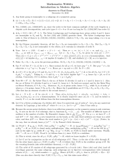
Define piecewise linear functions $1 and $2 on the unit interval
by
14
--I
and
Note that
i
I
= 1,2.
~i(l)
= 1,
~~(l)
= ~~(l),
and for s£[O,l],
~i(s)
<
~i(s),
(Figure 1).
lr--------------~
_I
Figure 1.
Since m1
= 6 and m2 = 1/6,
~l(S)
=
~1
~2
and
become
(1 - 6) + 6s
and
o
~2(s)
= {
,s<1-6
-1-1
(1 - 6
) + 6
s, s
>
1 - 6.
Define a new random walk {y } on the unit interval as follows:
n
let YO'" sO' and
Yn+1 =
~V (Y ),
n
n
I
I
I
I
I
I
I
n = 0,1,···.
I
I
I
I
I
I
-.
I
I
I.
I
I
I
I
I
I
I
I
15
We then obtain
0'
••
I
,
< E P
r
n-l
=1 P
P
rO r1
••• p
tV
(IjIr
( •• eljJr (SO)··
r n _ 1 r n-l
n-2
0
P ••• p
IjI
(1jI
(."1jI (<j>
(s»
r
r
r
r
r
0
o r1
n-l n-l
n-2
1
0
..
.»
·»
< •••
< E P
P
rO r1
••• p
r
<j>
n-l
r
(<j>
n-l
r
( ... <j>
n-2
r
(s ) ••• »
0
0
n=O,l,·· ••
Consequently, if lAm EYn = 1, it follows that
that lim IT (sO) = 1.
n
n
Since the limit of IT
l~m
EX = 1, and thus
n
is independent of s for
n
s£[O,l), we would have, in particular, lAm ITn(O) = 1
(i.~.
thus want to determine conditions under which lim EY
= 1.
n
n
q = 1).
We
Returning to the random walk {Y }, let us assume that So
n
for an arbitrary nonnegative integer i.
Ie
I
I
I
I
I
I
2
•• err
= r
IjIl (1 -
ej )
= 1 -
Since
ej +1 ,
j
= 0,1,·"
(7.2)
and
j
ej-l ,
°
j = 1,2,·",
the state space of the random walk{Y lis the set of all real numbers of
n
the form 1 - ~,
j
= 0,1,···.
Define a process W,
n
n = 0,1,···, as follows:
W = log (1 - Y ),
n
n
e
let
n = 0,1,···.
Hence we have
P(Wn
j) = P(Y
n
= 1 -
ej ),
n,j
=
0,1,· ...
16
From the definition of the Y - process and (7.2), it follows that {W }
n
n
is a random walk on the nonnegative integers with matrix of transition
probabilities
Pz
PI
0
0
0
pz
0
PI
0
0
0
Pz
0
PI
0
...............
....
This is, of course, immediately recognized as the classical random walk
on the nonnegative integers with a reflecting barrier at zero.
It is well known that the states of the Markov chain {W } are
n
positive recurrent if and only if Pz > Pl.
~
If PI
Pz, it follows that
for an arbitrary positive integer N,
P (Wn e:{ 0 , 1 , ••• , N }) -+ 0
as n
--+
n
n
-+
1 in probability, and, by bounded convergence, EY
n
It follows from the remarks above that q • 1 for PI
~
-+
1.
1/2.
We next want to investigate the nature of the arithmetic mean
and the geometric mean
in this example under the condition that PI
~
1/2.
_I
I
I
I
I
I
I
I
I
_I
CXl.
Consequently, in the Y -process,
Thus Y
I
I
I
I
I
I
I
-.
I
I
I.
I
I
I
I
I
I
I
I
Ie
I
I
I
I
I
I
.I
17
For the geometric mean, we have
e2p I -I ,
I
m PI m P2 = ePI ePI 2
l
so PI
~ 1/2 if and only if ml PI m2P2
<
1.
For the arithmetic mean, we
have
so m > 1 if an d on 1Y ].·f Pie 2 + (1 - PI ) > e, t h at is, i f an d on 1 y if
PI(l - e 2 ) < 1 - a.
PI < 1/(1 + a).
Hence for 0 < e < 1, m
But 1/(1 + e)
>
>
1 if and only if
1/2 for 0 < a < 1, so for PI in the
non-empty interval [1/2, 1/(1 + a)], the arithmetic mean is
the geometric mean is
although IT'(l) = mn
n
<
-+ ~
>
1 while
Hence for P I E[1/2, 1/(1 + a)], ITn(O)
1.
as n
-+
1
-+ ~.
We can now justify the statement that Theorem 4.1 cannot hold in
general for the m unequal and m > 1, for if, while m > 1, the geometric
r
mean is
<
-
martingale
1,
{~
~
n
n
= Zn /mn
-+
E~
0 with probability one, but
n
= 1, so the
} cannot converge in mean square, or even in the mean
(order one).
Case II.
e
Suppose there exists a real number a, 0 <
<
1, satisfying
the conditions
The last condition is, of course, equivalent to PI
<
P2 , or PI
<
1/2.
In this situation, we want to construct piecewise linear functions
with desired properties which bound
~I
and
~2
above.
To obtain the
required functions, choose an integer NI sufficiently large that
(1 -
e) +
as >
~I(s),
for s
~
1 -
NI
e ,
18
and an integer N2 sufficiently large that
(1 - a
-1
-1
) + a s > $2(s), for s
>
Then choose N or N still larger, if necessary, so that
1
2
N1 + 1
= N2 -
1
= N,
say.
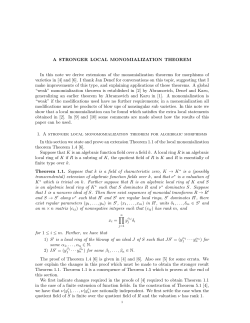
Now define piecewise linear functions
~1
and
~2
on the unit inter-
val by
s < 1 _ aN- 1
N-l
{ (1 - a) + as, s > 1 - a
I
~1(S)
=
aN,
and
The relationship of
~1
and
~2
to $1 and $2 is of the form described in
Figure 2.
I
.-I
I
I
I
I
I
I
I
_I
Figure 2.
Define the dual process {X } and the Y -process determined by
n
and
~2
as before.
n
In this case it is again easily seen that
~1
I
I
I
I
I
I
-.
I
I
I.
I
I
I
I
I
I
I
I
Ie
I
I
I
I
I
I
.e
I
19
EX < EY,
n n
n
= 1,2,···.
The Y -process is again a random walk on the
n
space of all points of the form 1 - aj ,
initial point So is of this form.
So
=1
-
ai
= 0,1,···,
j
provided that the
If, however, we assume that
for some i
>
N,
then the state space of the Y -process is the set of all real numbers
n
j ~
N.
We define
n
= 0,1,···,
so that
= P(Yn = 1
-
aN+j ),
n,j
= 0,1,···.
The W -process is again the classical random walk on the nonnegative
n
integers with a reflecting barrier at.zero.
Since P2 > PI (by assumption), the states of the Wn-process are
positive recurrent, and therefore a stationary distribution {u } exists.
j
In particular
P(Yn
as n
-+~.
=1
Hence for all n > no' say,
from which it follows that
for n
~
nO.
Thus
lim E(Yn Iyo
n~
=1
i
- a )
<
1,
20
.'I
and
= c,
It follows that lim ITn (s)
say, for c < 1 and s£[O,l); in particular,
lim IT (0) < 1, so extinction is not almost certain.
n
To sum up the results of this section, we have seen that:
(1)
m
= Pl ml + P2m2
q < 1, (3)
ml
=
a, m2
=
a
-1
m1
(PI < 1/2) implies q < 1.
>
= 1,
m > 1 and m > 1 implies
2
1
for adO,l) and aPI a- P2 ~ 1 (PI ~ 1/2)
~ 1 implies q
implies q .. 1, and (4)
a, m2
>
(2)
a-1 for a£(O,l) and aPI a- P2
>
1
The assumptions in (1) - (4) are not, of
course, exhaustive, but consideration of these special cases has shown
that the arithmetic mean m is not a critical parameter in determining
whether extinction occurs with probability one.
These cases suggest,
however, that the geometric mean (m 1P1 m2P2 for two environmental
states) is a critical parameter, as indeed we shall prove in Section 9.
8.
I
The Lindley process
In Section 9, the W -process is much more general than the classin
cal random walk of the special cases in Section 7; this section is
devoted to a discussion of the more general random walk which we will
encounter in Section 9.
The results of this section are due to Lindley
(1952), who introduced the process in connection with a waiting-time
problem in queueing theory.
could be applied to random
He also indicated that the methods employed
w~lks
of the kind encountered in the next
section.
Let Ul,U2'··· be a sequence of independent, identically distributed
random variables with Elull finite.
I
I
I
I
I
I
I
_I
I
I
I
I
I
I
-,
I
I
I.
I
I
I
I
I
I
I
I
Ie
I
I
I
I
I
I
.I
21
Define a sequence of random variables W,
n
n = 1,2,···, as follows:
Wo = 0, and
= wn
W
{ 0,
n+l
+ Un+1 '
n + Un + 1
if W
> 0,
n =
0,1,···.
(8.1)
if W.
+ Un + 1 -< 0,
n
The sequence {Wn } of nonnegative random variables will be called the
Lindley process.
The process also has the representation
W = max(O, U , U + U ••• U + U +...+ U )
n-l
n'
, 1
2
n '
n
n
For clearly WI = max(O, Ul).
and if W + U +
r
r
<
1 -
= 1,2,···.
Suppose (8.2) holds for n = r.
max(O, U ,U 1 + U ,
r
rr
=
n
0, Wr+l =0.
Then if
U + U +...+ U ) + U
1
2
r
r+l
Combining these two possibilities in
the single expression
it follows, by induction, that (8.2) holds for all n.
For x
~
(8.2)
0, we have
Since the U 's are independent and identically distributed, we may
n
renumber them without affecting the right hand member of (8.3); in
particular, if we replace Ur by Un
+1 ' r = l,···,n, we obtain
-r
P(Wn < x) = P(UI < x, U1 + U2 < x···
U + U2 +...+ Un < x).
'
, 1
22
If we write S
r
r
= S=1
r
U, this becomes
s
P(W
n
<
x) = P(S
<
r -
x for all r
_<
n).
(8.4)
We now want to establish the existence of a limit for F (x)
n
= P(Wn
<
x)
as n tends to infinity, for any x.
If E (x) is the event
n
= 1,2,···,
the sequence of events {En (x)}, n
for fixed x, is decreasing
and tending to the limit event
E(x) :
S
r
<
x for all r
>
1.
Hence by a property of probability measures,
lim Fn (x) = n~
lim P(En (x»
= P(E(x»
n~
exists.
If we denote this limit by F(x), then since
F(x)
= P(Sr
~
x
~or
all r
~
1),
it follows that F(x) is a nonnegative, nondecreasing function with
F(x)
= 0 for x
<
= P(Wn
0 (since F (x)
n
< x)
-
The question immediately poses itself:
F(x) a distribution function.
= 0 for x
<
EUl~.
under what conditions is
There are three cases to consider accord-
By the strong law of large numbers,
lim Sn In
n~
with probability one.
= EUI
Hence with probability one, for any sequence
{Ul, U2,···}, there exists no such that Sn > nEU1/2 for n
~
no'
follows that for x >.0, there exists a random no(x) such that
Sn > x for n
~
no(x)
••I
I
I
I
I
I
I
I
_I
I
0).
ing to the value of EUI'
(i)
I
It
I
I
I
I
I
-.
I
I
I.
I
I
I
I
I
I
I
I
Ie
I
I
I
I
I
I.
I
I
23
with probability one.
Thus F(x) =
pewn
x)
<
° for all x;
0, as n
~
that is
~ ~,
for all x.
(ii)
EU,
<
Again by the strong law of large numbers,
0.
lim Sn /n = EUI
n~
with probability one.
Given
E >
0, it follows by Egoroff's theorem
that there exists an integer nO such that
P(Sn ~
° for all n
~
(8.5)
no) > 1 - E/2.
Further, considering the joint distribution of SI, S2,"', S , we can
no
choose x sufficiently large that
peS
< x for all n < no) > 1 - E/2.
(8.6)
n -
From (8.5) and (8.6), we obtain
peS
n
x for some n
>
1) <
>
E,
that is,
F(x)
= peSn
for sufficiently large x.
l!m
F(x)
= 1.
x for all n
<
-
Since
l!m
F(x)
>
~
1)
>
1 -
E
1, it follows that
Thus in this case the existence of a nondefective
limiting distribution function has been established.
(iii)
and EUI
= 0,
EU,~.
Chung and Fuchs (1951) show that if E!Ull < ~
then for arbitrary
p(ls
n - xl <
E
E >
0, and any real number x,
infinitely often)
= 1,
unless all values assumed by Ul are of the form iA (i
(8.7)
= 0,±1,±2,"')
for A a real number, in which case (8.7) holds for every x of this form.
24
The case where U1 = 0 with probability one is excluded.
= P(Sn
F(x)
< x for all n ~ 1),
=0
i t follows inunediately that F(x)
be exceeded by S
n
Since
for all x since any value x will
for some n with probability one.
Hence we have the following result.
Theorem 8.1 (Lindley).
probability one.
-+ ~
is finite and U1 is not zero with
Then a necessary and sufficient condition that the
distribution function Fn (x)
as n
Elu 1 1
Suppose
is that EU 1
O.
<
= peWn
x) tends to a nondefective limit
<
If EU 1 > 0, P(Wn
<
x) tends to zero for
any x.
9.
Conditions for almost certain extinction
Theorem 9.1
Suppose r. p Ilog m
r r
r
(a)
If E p
(b)
If
r
t
r
I
log m < 0, then II (0)
r
Pr log mr
n
>
E Pr log(l -
-+
q < 1 as n
-+
1 as n
~
r
(0»
(9.1)
converges,
-+ ~.
We have not determined whether the condition (9.1) is necessary,
but have been unable to obtain the result without it.
We can, however,
remove all conditions if there are only a finite number of environmental states (Corollary 9.1).
Proof of Theorem 9.1.
Let {V } be the environmental process consisting
n
of independent, identically distributed random variables with probability
mass function {p }, and let
r
{~
r
(s)} be the corresponding sequence of
probability generating functions with
~~(l)
= mr ,
r
= 1,2,···.
.-I
I
I
I
I
I
I
I
_I
-+ ~.
0, and
r
then II (0)
n
< ~.
I
Let
I
I
I
I
I
.-I
I
I
I.
I
I
I
I
I
I
I
I
Ie
I
I
I
I
I
I.
I
I
25
{x }
n
be the dual process of Section 6, for which
(9.2)
for soE[O,l).
(a)
rE Pr log mr -< 0.
Theorem 5.1,
IT
n
(0)
-+
If m = 1 for all r, then m = 1 and by
r
Thus we shall henceforth assume that m f 1
r
1.
for some r.
Define two subsets of the positive integers by
M
= {r: mr
1
<
I}
and M2 = {r: m > I}.
r
We then define piecewise linear functions
~,
r = 1,2,'··, on
r
the unit interval by
~ (s) =
r
(1 - m )
r
+ mr s
, rEMl
and
(9.3)
s < 1 - 11m ,
~
Then
~
r
(1) = 1,
r
r
(s)
~'(1)
r
+ mr s, s
11m,
r
> 1 -
= $'(1), and, for sE[O,l],
r
~
r
rEM 2 •
(s) < $r(s),
r=!,2,···.
Based on these functions
the unit interval as follows:
Y
n+l
Then
< •••
~r'
define a process Yn ,
YO =
° and
n
= 0,1,···.
n = 0,1,···, on
26
(9.4)
=1 -
If we write s
1/J
r
(1 - e
=
-x)
e- x
x > O. the equations (9.3) become
{II - eO-(x-log m )
- e
x - log m
<
0
r • x - log m
>
O.
r
(9.5)
r -
Define
Wn
= -log(l
- Yn ).
= 0.1.···.
n
from which it follows that
peW
<
n -
x)
= P(Yn
<
1 - e- x ). x
>
O.
11
= 0.1.···.
Define a sequence U1. U2,··· of independent. identically distributed.
random variables by
Un • -log
nvn-1 .
n •
0
- e-(Wn+Un+ 1) , W + U
> O.
n
n+1
by (9.5).
Hence
= -log(l
- Y )
. n+1
=
o
, Wn +U+
n 1 <0
{W + U
that is, {Wn } is a Lindley process.
n
I
I
I
I
I
I
I
I
I
I
I
I
Then
<
.-I
_I
1.2.···.
, Wn + Un+l.
I
n+1' Wn + Un+ 1
~
0,
.-I
I
I
27
~
I
I
I
I
I
I
I
I
Since
-L P log m > 0,
r r
r
it follows from Theorem 8.1 that
P(W
<
n -
I.
I
I
-+
0 for all x > 0, as n
-+ ~.
Hence
P(Y
<
n -
that is, Yn
-+
1 - e-xlY
o
= 0)
-+
0 for all x > 0, as n
1 in probability, given YO = O.
-+
1, and thus by (9.4), E(Xn Ixo = 0)
(9.2), ITn(O)
-+
1 as n
~-2r
(b)
-+~,
-+
~,
By bounded convergence,
E(Y n Iyo = 0)
-+
1.
Finally, by
so extinction occurs with probability one.
Suppose L P log m = a > O.
r r
r
log mr > 0 and (9.1) holds.
Choose nO sufficiently large that
Ie
I
I
I
I
I
x)
n
L p log mr > a/2 for n -> nO'
r=l r
Since
~
Pr log(l -
~r(O»
converges, we can choose N > no sufficiently
large that
I r>L p r log(l - ~ r (0»
N
I
< a/2.
It follows that
N
L p log mr + r>EN p r log(l r=l r
There exists
£,
0
< £ <
1, such that
~
r
(0»
> O.
28
that is,
N
rli 1
Let
m~
= emr ,
Pr log(em r ) + r~N Pr log(l - ~r(O»
r - 1,···,Nj
m~
~r(O),
= 1 -
>
O.
(9.6)
r - N+l,···, so that
(9.6) becomes
rL Pr log m'r > O.
(9.7)
We note that
Therefore, mr > 1 -
~
r
(0) for all r, and, in particular, for r > N.
Thus since m' < m for all r,
r
r
sufficiently close to 1.
~
r
(s) < (1 - m') + m's for s .. s(r)
r
r
For each r .. 1,···,N, let t
r
< 1 be the
smallest nonnegative real number such that
(1 - m') + m's >
r
r -
= max {(I -
and let t
m') + m't,
r
r r
~
r
(s) for s
>
r = 1,···,N}.
Define piecewise linear functions
~l' ~2'···
Clearly 0 < t < 1.
on the unit interval
Thus
~
r
C
s < [m' - (1 - t) ] 1m' ,
r
r
r .. 1,2,···.
(9.8)
- m') + m's
(s) <
-
~
r
r
s > [m' - (1 - t) lim' ,
r
r '
r
(s) for 0 < s < 1 and r .. 1,2,···.
--
Define a process Yn , n .. 0,1,···, on the unit interval as follows:
Yo
=
1 - e
110g(1-t)1= 1 _ e -a • say, and
n
= 0.1,···.
.-I
I
I
I
I
I
I
I
el
t ,
r
by
~ (s) =
r
I
I
I
I
I
I
.-I
I
I
I.
I
I
I
I
I
I
I
I
Ie
I
I
I
I
I
I.
I
I
29
In this case, we have E(X
n
Ix o =
a
1 - e- ) < E(Y IYo = 1 - e- a ).
With the representation 1 - e
-
-x
, x
~
n
0, for real numbers in the
semi-closed interval [0,1), the equations (9.8) become
-a
x - log m' < a,
x
$ (1 - e- ) = {l - e_(X_10g m')
r
r
1 - e
r
r
= 1,2,···.
(9.9)
x - log m' > a,
r -
Define
Wn
=-
log(l - Yn ) - a,
n=O,l,···,
from which it follows that
°
peWn-< x) = P(Yn-< 1 - e -(x+a» ,x~,
= o,1,···.
n
Define a sequence U1, U2,··· of independent, identically distributed
random variables by
Un
=-
log ~
,
n-1
n
= 1,2,···.
Then
Y
n+1
=
1 - e
-a
,Wn +U+
<0
n 1
{ 1 - e -(Wn+Un+ 1+a) , W + U
> 0,
n
n+1
by (9.9).
Hence
W
n+1
=-
log(l - Yn+ ) - a
1
Wn + Un+1 <
W
n
that is,{W } is a Lindley process.
n
+ Un+1
°
> 0,
30
Since
= -
L p
r
r
log m' < 0
r
by (9.7), it follows from Theorem 8.1 that the W -process has a nonn
defective limiting distribution.
That is,
lim lim P{W
For some e, 0
<
e
<
<
n-
~ n~
x)
= 1.
(9.l0)
1, choose x o sufficiently large that
lim P{W < x o) > e,
n:;<iO
n -
and then choose nO sufficiently large that
Thus we have
P{Yn
<
1 - e-{xo+a) IY o
=1
/2o
fr n
- e -a) > e
~
nO'
It follows that
E{Y IYo
n
=1
- e- a ) < (e/2)[1 - e-{xo+a)] + (I - e/2)
=1
- (e/2)e
-(xo+a)
~
, for n
nO'
Since the right side of this inequality is independent of n,
lim E{Yn IYO = 1 - e
n:;<iO
-a
) < J..
We therefore obtain
< n-+<>o
lim E{Yn Iyo = 1 - e
< 1 .
-a
)
I
.-I
I
I
I
I
I
I
I
_I
I
I
I
I
I
.-II
I
I
I.
I
I
I
I
I
I
I
I
Ie
I
I
I
I
I
I.
I
I
31
It follows that for all s£[O,l), and in particular s
=
0, lim IT (s)
and extinction does not occur with probability one.
The proof of the
n
<
1
theorem is complete.
The following results follow immediately from Theorem 9.1.
N
Corollary 9.1.
If, for some positive integer N,
r~l
Pr = 1, then a
necessary and sufficient condition for extinction with probability one
is that L p log m < O.
r r
r Corollary 9.2.
If L p [log m
r r
r
c < 1 such that
~r(O) ~
10.
I
00, L p log m > 0, and there exists
r r
r
c for all r, then ITn(O) -+ q < 1 as n -+ 00.
<
Comparison with related processes
It is interesting to compare the branching process in a random
environment with two related branching processes which may be classified as multitype Galton-Watson processes, the latter being generalizations of the simple Galton-Watson process to processes involving several
different types of objects.
the multi type
Before introducing these two processes,
Galton-Watson process will be defined and those pro-
perties of interest here will be stated.
For a detailed discussion of
the multitype Galton-Watson process, the reader is referred to Chapter II
of Harris (1963).
We will consider a multitype process consisting of k types (k < 00).
Associated with type i is the probability generating function
=
r
l'
00L
P i (r . •. r ) s rl ... s rk
. .. r =0
1"
k 1
k'
'k
lSI
I, ... , Isk I
< 1,
i = l,"·,k,
(10.1)
32
where p i (rl,···,r ) is the probability that an object of type i has
k
r
l
offspring of type 1, r
Let
of type 2,"', r
Z
~ = (Z~"",Z~)'
If ~
the nth generation.
r l + ••• + r
k
k
of type k.
represent the population size, by type, in
=
(rl,"',r k )', then ~+l is the sum of
independent random vectors, r l of them having the generating
function fl, r 2 of them having the generating function f2,"', r of
k
k
If Z
them having the generating function f .
i
fn(Sl,"',sk) =
i
fn(~
-.l
= -0,
then Z +1 • O.
-.l
represents the generating function of
-
~,
If
given
a single object of type i in the zeroth generation, then
n
= 0,1,'"
(10.2)
i=l,···,k,
or, in vector form,
(10.3)
I
.-I
I
I
I
I
I
I
I
_I
Let M = (m
ij
) be the matrix of first moments
i,j = 1,"',k,
where
~
(10.4)
denotes the column vector whose ith component is 1 and whose
other components are O.
E(Z
Then
+mlz ) = z' MM,
-.l
-.l
-.l
n,m
= 0,1,"',
with probability one, and, in particular,
E(zlz
'-=n -0
the ith row of
MF.
= =:t.
e ) = e'
=:t.
MF '
(10.5)
I
I
I
I
I
.-I
I
I
I.
I
I
I
I
I
I
I
I
Ie
I
I
I
I
I
I.
I
I
33
We shall call a vector y or a matrix A positive (y
>
Q, A
>
0) or
nonnegative (v > 0, A > 0) if all its components have these properties.
- - -
If
~
-
and yare vectors, then u
>
y
(~ ~
v) means that
~
- y
0
>
The basic theorem concerning extinction with probability one can
We shall assume that ~ is positive for some positive
now be stated.
integer N.
The process is then said to be positively regular.
a matrix has a positive characteristic root p
which is simple and
greater in absolute value than any other characteristic root.
also assume that the process is not singular.
Such
2
We shall
(The process is said to
k
be singular if the generating functions f1(sl'···' sk)' ••• , f (sl' .··,sk)
are all linear in sl'···' sk with no constant term.)
Let qi be the
probability of extinction if initially there is one object of type i;
that is,
qi
= P(~ = Q for
some
The vector (q1, ••• , qk )' is denoted by
s.
nl~o = ~).
Let
1 denote the vector
(1,1, ... ,1)' •
Theorem 10.1 (Harris).
not singular.
If p
~
Suppose the process is positively regular and
1, then S
= 1.
If P > 1, then 0
~
S < 1, and S
is the unique solution of the equation
(10.6)
satisfying
Q~
~
< 1.
2 If ~ > 0, the matrix M must be irreducible, since every power of
a reducible matrix is reducible. The result now follows from the
Frobenius Theorem [Gantmacher (1959), p. 65].
34
We now want to define two multitype Galton-Watson processes of a
k
Let {Pi} be a probability mass function with i~l Pi = 1
special type.
for some positive integer k and let
{~i(s)}
be a corresponding sequence
of probability generating functions satisfying the assumptions of
= L PijS j is the probability generating function for
Section 1; ~i(s)
the number of offspring of an i-type object.
A-process.
In this process, we shall assume that all offspring of
an object of type i are of the same type, type j with probability Pj'
j
= l,···,k.
That is, in the notation of (10.1),
pi(O, .. • , 0)
=
pi(O,···, 0, r ,
j
pi(r
1'
...
,
r )
k
o, ..• ,
0)
PiO
PjPir
=
j
j = l,·",k;
r
j
>
1
0, otherwise.
Then
I
.-I
I
I
I
I
I
I
I
_I
and, by (10.2),
(10.7)
The matrix M of first moments is given by
M =
••••••••••••••••••••••
II
•
I
I
I
I
I
..-I
I
I
I.
I
I
I
I
I
I
I
I
Ie
I
I
I
I
I
I.
I
I
35
B-process.
In this process, we shall assume that each offspring
of an i-type object is of type j with probability p., independently of
J
the type of other offspring (and of the type of the parent object).
k
If r
= j~l
r j , then, in the notation of (10.1),
Thus
f
ie s l ' ... ,sk)
and
(10.8)
The matrix M is the same as in the A-process.
Since these two processes have the same moment matrix M, they both
become extinct with probability one if and only if p
~
1.
Now it is a
well-known result of matrix theory that if C is a nonsingular matrix,
then M and C-1MC have the same characteristic roots.
let
o
C
=
...
o
o
.
.
o
o
o
...
Therefore, if we
36
then
Hence P - Plml + P2 m2 +••.+
Pk~'
since the dominant root of a non-
negative matrix cannot be greater than the maximum row sum nor less than
the minimum row sum [Gantmacher (1959), p. 82].
Thus, if
p >
1, we have by (10.6) that the probabilities of extinc-
tion satisfy
(10.9)
i-l,···,k,
for the A-process, and
i - l,···,k,
(10.10)
i
n
i
n
Using an induction argument, i t is easily seen that Bf (Q) < Af (Q)
-
for i = l,···,k, from which we obtain ~B ~ ~A (~.~., q~ < q~ for
i = 1,···,k) .
we let
~O
=~
~O
is nonrandom in the A- and B-processes.
with probability Pi'
Suppose
i - l,···,k, so that these pro-
cesses are more analogous to the random environment process defined by
{Pi} and
{~i(s)}.
We still obtain extinction with probability one if
and only if p < 1, and in case p
is given by
.-I
I
I
I
I
I
I
I
el
for the B-process.
We recall that
I
>
1, the probability of extinction
I
I
I
I
I
.-I
I
I
I.
I
I
I
I
I
I
I
I
37
for the A-process, and
for the B-process, with qB
~
qA.
Let f (s) be the probability generating function for the size of
n
the n!h generation, without regard to type, in the A-process with Zo
random
Zo =
(i.~.
~
with probability Pi'
f
n
(s)
k
= i=1
L
P
i
f
i
n
i = 1,···, k).
Then
(s,···, s).
(10.11)
From (10.7) we obtain
i
k
i
<
il~1 i2~1
f n W = i ~1 Pi 4>i (f n _1 1 (§.»
1
1
k
k
i
Pi Pi/i (4)i (fn~2 W»
1
1
<
Ie
I
I
I
I
I
I.
I
I
Therefore, from (10.11),
f n (s) < i i
, l'
=
by (2.2).
k
...L.~
'n-l
=1
II (s)
n
In particular, fn(O)
~
IIn(O) , so qA
~
q where q is the
probability of extinction in the random environment process.
We note that if Plm l +...+ Pk~ > 1 while mil m~2 •••m{k ~ 1, the
random environment process becomes extinct with probability one, while
38
the A- and B-processes (with
~O
random or non-random) have a positive
probability of surviving indefinitely.
The results of this section may be summarized as follows.
Theorem 10.1
If p
.Q.
~
(a)
Suppose
= Plml +..•+
~
SB
SA <
~;
Pk~ ~
=~
~o
(non-random).
1, then SA
= SB
=~.
If p
>
1, then
SA satisfies the equations
i • l,···,k,
and
satisfies the equations
~
i =
(b)
Suppose
If p
~
~O
=~
with probability Pi'
1, then qA • qB
=q =1
~
~
q
i
1,···,k.
(10.13)
= l,···,k.
(q is the probability of extinction in
the random environment process).
qA
(10.12)
If p > 1, then 0
~
qB
~
qA < 1 and
1, where
and
i
i
with qA and qB (i
= l,"',k)-
given by (10.12) and (10.13) respectively.
I
.-I
I
I
I
I
I
I
I
_I
I
I
I
I
I
.-I
I
I
I.
I
I
I
I
I
I
I
I
Ie
I
I
I
I
I
CHAPTER III
EXTINCTION PROBABILITIES
11.
Introduction
In the classical types of branching processes, in which distinct
objects reproduce independently, the iterative nature of the probability
generating functions for the sizes of successive generations often leads
to equations such as s = f(s) or
extinction probabilities.
which are satisfied by the
Further, given the probability of extinction
ql' say, with one initial object, it follows from the assumption of
independence between objects that the probability of extinction with j
initial objects, say qj' is simply qj
= q{.
not exist in the random environment process.
Such a relationship does
In this chapter, we
determine bounds for these probabilities.
We shall occasionally require the conditions in Theorem 9.1, and
therefore state them here for reference:
L Pr Ilog mr
r
12.
I
< ~,
rL Pr Ilog mr
I
L Pr log mr
> 0,
r
< ~,
rL Pr log mr -< 0;
L p r log(l - ~ r (0»
r
(11.1)
converges.
(11.2)
Moments of the dual process
Let n(k)(s) designate the generating function of Z , given that
n
n
Zo = k, n = 0,1,···, k = 1,2,···.
I.
I
I
~ = i(~),
nn (s).
For n(l)(s) we shall simply write
n
40
rr(k)(s)
n
= rI:
P
r
rr(k) (CPr(s»,
n-l
n = 1,2,···; k = 1,2,···,
(12.1)
The proof is analogous to the proof of Theorem 2.1 and will be
omitted.
From (12.1) we obtain
= mn
rr(k) , (1) ... mrr(k) , (1)
n
n-l
rr(k) '(1)
0
= kmn •
By repeated application of (12.1), we obtain the representation
rr(k)(s) ...
p p ••• p
r •••I: r
r _
n
0'
'n-l r O r 1
n 1
cP
k (CP ( .... cp
(s)···».
rO r1
r _
n 1
(12.2)
We shall also state, without proof, the following theorem, which
is analogous in statement and proof to Theorem 3.2.
Theorem 12.2
For s£[O,l),
We next want to establish
a relationship between rr(k)(s)
and the
.
n
n
=r
One obtains for the kth moment of X , given
n
0'
..•I: r
,
.-I
I
I
I
I
I
I
I
el
where qk is the probability of extinction, given Zo = k.
dual process {X}.
I
n-l
P r P r ••• p r
o
1
A..
n-l
k
~r
(A..
0
~r
( • • • A..
1
~r
n-l
(s ) •••
0
»'
I
I
I
I
I
II
e
I
I
I
I.
I
I
I
I
I
I
I
I
Ie
I
I
I
I
I
41
so from (12.2) we have
(12.3)
From (12.3) and Theorem 12.2, we obtain
Theorem 12.3
(at the n!h step) tends to a limit, which is the probability of extinction for the random environment process (the Zn -process), given k
objects in the zeroth generation, k
= 1,2,···.
That is,
= 1,2,···.
for sO£[O,l) and k
It follows [Feller (1966), p. 244] that there exists a random
k
variable X such that X tends to X in distribution and qk = EX is
n
the kth moment of X. We shall refer to this limiting distribution as
the ergodic distribution of the dual process.
Under the assumptions o£ Theorem 9.l(b), and with {Yn } and {Wn }
defined as in its proof, it follows that
Hence
= x~
lim
by (9.10).
I.
I
I
As n tends to infinity, the kth moment of the dual process
Given £
lim P(X
n~
n
>
lim P(Wn < xlwo
n.:;<i)
= 0)
1,
0, choose x o sufficiently large that
< 1 - e-(xo+a)lxo
=1
- e- a )
>
1 - £.
(12.5)
42
Let G be the distribution function of X on [O,ll; that is, G is the
ergodic distribution of the dual process.
k
G(l-)
= 1.
qk
0 as k
-+
By (12 .. 5) i t follows that
Hence by bounded convergence, EX
-+
-+
0 as k
-+
=; that is,
=.
We may summarize these results as follows.
Theorem 12.4
To any branching process {Zn } in a random environment
(as defined in Section 1). there corresponds. on the unit interval, a
dual Markov process {X } (as defined in Section 6), possessing an
n
ergodic distribution G, the kth moment of which is the probability qk
that the branching process becomes extinct, given that Zo
= k.
Furthermore. if (11.1) holds,
1
qk
=f
o
x
k
dG(x)
=1
for all k
= 1,2,"',
qk =
13.
fo
k
x dG(x)
~
0
as k
-+
=.
Equations for extinction probabilities
We shall assume, in this section, that the conditions (11.2) are
satisfied.
Let
i
= 0,1,"',
k
= 1,2,"',
so TI~k)(s) can be written in the form
(k)
TIl
(s)
=
= i~O
.-I
I
I
I
I
I
I
I
_I
while if (11.2) holds,
1
I
(k)
Pi
i
s,
Is I
< 1,
k
= 1,2,···.
(13 .1)
I
I
I
I
I
.-I
I
I
43
I.
I
I
I
I
I
I
I
I
q1 =
p~l)
~ + •••
+ pP) q1+p~1) q 2 +"'+p(1)
n
q2 = p~2) + P1(2) q1 + p~2) q + ...+ p(2)
2
n
~
+ ...
(13.2)
q = Po(n) + P1(n) q1 + p~n) q + ...+ P (n) qn +...
2
n
n
We can write the first n of equation (13.2) as
+ (1) q + ••• + P ( 1)
+ C( 1)
P1
q1 = P~ 1)
qn
1
n
n
(2) + (2) q + ••• + p(2)
q2 = Po
P1
1
n
~=
Let Y , j
j
~ + C~2)
(13.3)
(n) + (n) q +"'+p(n)
+ C(n)
qn
Po
P1
1
n
n
= 1,2,"',
be a decreasing sequence of real numbers
tending to zero, and such that
Ie
I
I
I
I
I
I
I
I
We then have the system of equations
q
j
= EXj
< Y
j'
J'
= 1,2,···.
It then follows that
(13.4)
Let
(1)
P1
An
=
(2)
P1
(n)
P1
-
If
~j(O)
= 0
trivial.
If
(n)
P2
for all j, then q1 = q2 = ••• = 0, and the problem is
~j(O)
> 0 for some j, then
p~k)
> 0 for all k
= 1,2,"',
44
and it follows that An is a nonnegative matrix whose row sums are all
less than 1 (for any n).
From the theory of nonnegative matrices [Gantmacher (1959),
Chapter III], it follows that A has a nonnegative characteristic root
n
A such that no characteristic root of A has modulus exceeding A •
n
n
n
Further, if sand S denote respectively the minimum and maximum row
n
n
sums of A , then
n
s n <An<S,
- n
and, since Sn < 1, we have An < 1, whatever the positive integer n.
Let ~
C'
-n
=
=
(ql' q2"", qn)',
A)a
n-n
(E -
x
and
Equations (13.3) thus become
(C(l) C(2) ••• c(n»,.
n'n'
'n
where E .. E(n
.fn .. (p~l), p~2), ••• , p~n»"
= -n
P + -n
C ,
(13.5)
n) is the identity matrix.
Since An < 1, IE - Ani ~ O•. Hence (E - An )-l exists for all n,
and we have further [Gantmacher (1959), Chapter III] that
(AE - A )-1 > 0
n
. -1
In particular, therefore, (E - A)
n
Let R~j), j
from (13.4),
= l,···,n,
n
>
-
O.
.-I
I
I
I
I
I
I
I
_I
I
for A > A •
-
I
From (13.5), we thus obtain
denote the row sums of (E - A ).
n
Then,
,I
I
I
I
.-I'
I
I
I.
I
I
I
I
I
I
I
I
Ie
I
I
I
I
I
I.
I
I
45
(13.6)
Since (E - A )-1 is a nonnegative matrix,
n
(E - A)
n
-1
P < a < (E - A)
-n--n,n
-1
[P
-n
+ Yn+ 1 1L].
..
(13.7)
where R = (R( 1) R(2) ...
-n
n'n"
But R
-n
=
(E - A)l
n -'
where _1
=
(1 1 ···1)'
"
"
so (E - A )-IR
n
-n
= _1,
and
(13.7) becomes
(13.8)
Hence we have the following result.
Theorem 13.1
Y , j
j
Suppose the conditions (11.2) are satisfied.
= 1,2,···,
Let
be a decreasing sequence of real numbers tending to
zero and such that q.
J
= EXj
< y., j
J
= 1,2,···.
Then (13.8) holds for
all n = 1.2.···.
Theorem 13.1 shows that we can obtain any number of the qj'S to
any desired accuracy given a suitable sequence {Yj}.
(13.8) holds provided only that qj
decreasing
sequen~e.
= EXj ~
We note that
Yj and that {Y j } is a
However, the conditions (11.2) imply the existence
of such a sequence with Yj
+ O.
By using the first of inequalities (13.6), we can obtain upper
bounds on the qj'S which are better than those given by (13.8).
is, if T(j)
n
=
That
(1 - rio p;j»,then by the first inequality in (13.6),
46
=
It follows from (13.5), with T
-n
(E - A)
n
-1
(T(l), T(2) , ••• , T(n», , that
n
n
n
P < a < (E - A)
-n-"""'tln
-1
-1
P + Yn+l(E - A)
T.
-n
n-n
(13.9)
In one special situation, we can find a simple sequence {Y } as
j
the following theorem shows.
Theorem 13.2
r
= 1,2.···.
Suppose the probability generating functions
~
r
r
(s) < s,
(13.10)
for s > y.
(13.11)
for all n
= 1,2,···.
Note that (13.10) implies that m
r
>
1 for all r, and if there are
only a finite number of environmental states, then m > 1 for all r
r
implies (13.10).
Proof.
j
E(X Ixo = y) =
n
p
< r
l'
...L r
'n-1
p
Pr ."p
rO
r
1
•• 'p
1
r
r n- 1
~jr
~j
n-1
r
n-l
(~
n-1
< •••
Hence
so we may put Yj
= yj,
j -- 1 '"
2 •••
..
in (13 8)
r
(~r
n-2
(·"~r
(';'<jl
n-2
0
r
(y) ... »
(y) ••• »
1
.'I
I
I
(s),
are all such that for some y < 1,
~
I
I
I
I
I
I
_I
I
I
I
I
I
.-I
I
I
I.
I
I
I
I
I
I
I
47
Example.
Suppose there are just two environmental states.
~l(s) = t + ~ s2, ~2(s) = t s + t s2, and PI = P2 = ~.
~1(S)
that is, y
n(I)(S)
I
=
= t.
n(3)(S)
I
.12500 + .16667s + .70834s 2
=
.00782 + .07032s 2 + .01852s 3 + .32205s 4 + .22222s 5 + .35909s 6
n~4)(s) = .00196 + .02344s 2 + .111658 4 + .04939s 5 + .35909s 6 + .19753s 7
+ .25697s 8 •
With n
= 4,
A4
we have
=
.16667
.70834
0
0
0
.24306
.22222
.50347
0
.07032
.01852
.32205
0
.02344·
0
.11165
1.20000
1.17112
0.26517
0.75986
0
1.37777
0.31195
0.89392
0
0.11065
1.04392
0.44101
0
0.03635
0.00823
1.14925
and
I
I
I
s;
n~2)(S) = .03125 + .24306s 2 + .22222s 3 + .50347s 4
I
I
I
=
The equations (13.1) are given by
Ie
I.
In this example,
y in (13.10) is the solution less than 1 of the equation
I
I
Let
(E - A )-1
4
f.4 =
=
(0.12500, 0.03125, 0.00782, 0.00196), and y5
(13.11) we obtain
= 0.00412.
From
48
0.19016
0.19428
ql
0.04725
0.05137
q2
<
<
0.01249
q3
0.00345
q4
-
... ,
q4·
I
0.00757
The same procedure leads to the bounds
.19040 .
.04753
.19045
<
<
.04758
.01294
.01299
.00368
.00373
In taking n larger to improve the bounds on ql'···' q4' we also obtain
the lower bounds .00107, .00032, .00009, .00003 for q5'···' q8' respectively, each differing from the real value by less than y 9
14.
=5
x
10 -5 •
The case of two environmental states
In this section we shall assume that there are just two environ-
mental states, and that mil m;2 > 1 (~.~., extinction is not certain).
In Section 13, we obtained bounds on the qj'S in the case when all the
m 's are greater than 1.
r
ml
~
1 and m2 > 1.
Hence we shall further assume here that
In this case,
~e
obtain explicit bounds for the
moments of the ergodic distribution of the dual process and consequently
bounds on the sequence {qj} of extinction probabilities.
This will be
accomplished by "bounding" the dual process by a process of a very
special kind for which an equilibrium distribution exists and can be
obtained.
.-I
0.01661
Suppose we let n = 8 in (13.11) in order to obtain better bounds
for ql'
I
I
I
I
I
I
I
el
I
I
I
I
I
.-I
I
I
I.
I
I
I
I
I
I
I
49
We shall need the following result.
Lemma 14.1. If ml ~ 1, m2
I
I
I
I
I
1, and mil m~2
>
1, Pl + P2 = 1, then there
exist relatively prime positive integers a and b and a real number
o
<
a
<
1, such that
aa
<
a-b
ml ,
<
m2 , and aPl - bP2
<
a,
o.
Since xPl yP2 is a continuous function of x and y, there exists
Proof.
a spherical neighborhood N of (m l , m2) such that (x, y)eN implies
x Pl yP2 > 1. Let R = {(x, y) 10 < x < ml , 1 < Y < m2 }. There exists
(x, y)eNoR such that
log x
log(l/y)
where r is a rational number.
positive integers.
r > 0,
Let r
alb, for a and b relatively prime
Then
I
Ie
>
~ log x =
r
log(l/y),
that is,
x
Let
a = x l/a
andy
>
0
(~.~.
a
l/a = y -lIb .
is the positive real ath root of x), so x
= aa
= e-b .
Note that this is only an existence theorem and does not describe
a procedure for finding appropriate values of a, b, and
a.
However,
in practice, these can generally be found by trial and error without too
much effort.
We now proceed as in Case II of Section 7 to construct piecewise
I.
I
I
linear functions which bound
~l
and
~2
above.
By Lemma 14.1, there
50
exist relatively prime positive integers a and b, and a real number a,
o<
a
<
1, such
that a
a
< ml , a
-b
< m2 , and aPI - bP2 <
o.
To obtain the required functions, choose an integer NI sufficiently
and an integer N2 sufficiently large that
Then choose NI or N2 still larger, if necessary, so that
~2
= N2
- b - N, say.
Define piecewise linear functions
~l
and
on the unit interval by
~l (s) =
{I(1-
s < 1 _ aN-a
aN
_ aa) + aas, s > 1 - aN-a
_I
s < 1 _ aN+b
= so£[O,
Yn-process as usual with Yo = So and Y + =
n l
~V
n
1), and define the
(Yn ) ,
n = 0,1,···.
Then it easily follows that
k
k
E Xn -< E Yn ,
(14.1)
k
We want to show that n~
lim E y n exists for all k and tends monotonically
to zero as k
~~.
Since
a!m E X~ = qk'
we shall have
I
I
I
and
Let {X } be the dual process with Xo
n
.'I
I
I
I
I
large that
NI + a
I
I
I
I
I
I
.-I
I
I
I.
I
I
I
I
I
I
I
I
51
k
where Y
k
aN, then the state space of the Y -process is
n
N
j
the set of all real numbers 1 - a + , j = 0,1, ..•.
If we let s 0 = 1 -
The Y -process is a Markov chain with transition probabill ties
n
i,j,n = 0,1,···,
given by
(14.2)
Ie
I
I
I
I
I
I.
I
I
= 1,2,···,
Lemma 14.2.
Proof.
Pb,o
= P2 ' Pb,a+b
Pi,i-b
= P2 ' Pi,i+a = PI'
Pij
= 0,
PI
i
= b,b+l,···
otherwise.
The Markov chain {Y } is irreducible and aperiodic.
n
Once we have shown the chain to be irreducible, it follows
immediately that it is aperiodic, since POO > O.
To show that the chain is irreducible, we must show that every
state is accessible from any given state.
number 1 -
aN+i
every state.
as state i , i
= 0,1,···.)
(We shall refer to the real
Clearly 0 is accessible from
If the state 1 is accessible from the state 0, then every
state is accessible from 0 (and thus from every other state), so we have
only to show that 1 is accessible from O.
That is, we must prove that
52
there exist positive integers nand m such that
na - mb = 1.
The argument used is based on arguments in Hardy and Wright (1960)
employed in obtaining more general results in number theory.
Let S be the set of all integers of the form na - mb, where n and
m are integers (a and b are the given relatively prime positive
integers).
If sl' s2 eS , sl
s2
±
=
(n 1
±
n 2)a - (m 1
±
m )b e S, so S
2
contains the sum and difference of any two of its members.
Clearly S
contains positive integers; let d be the smallest positive number in
S.
If s is any positive number in S, then s-zd e S for every integer z.
Now if c is the remainder when s is divided by d, and
s
then ceS and
°
< c < d.
c = 0, and s = zd.
of the number d.
b, and therefore d
d
= 1,
= zd +
c,
Since d is the smallest positive number in S,
It follows that S consists of integral multiples
Since d divides every number in S, it divides a and
~
1 (since a and b are relatively prime).
and hence S consists of all the integers.
solution of na - mb = 1.
large that n
1
= nO +
That is,
Let no' m be a
O
Let r be a positive integer sufficiently
rb and m
1
= mO +
ra are both positive.
Then
n 1 a - m1b - noa - mob = 1,
so (n , m ) is a solution with positive integers.
1
1
It follows that the
state 1 is accessible from the state 0, and the proof of the lemma is
complete.
An irreducible aperiodic Markov chain is positive recurrent if the
equations
k
= 0,1,'"
I
.'I
I
I
I
I
I
I
I
el
I
I
I
I
I
.-I
I
I
I.
I
I
I
I
I
I
I
I
Ie
I
I
I
I
I
53
have a solution {~} (~ not all zero) satisfying LI~I
00.
Further-
more, such a solution is a scalar multiple of the unique stationary
distribution {w } for the chain.
k
Thus, in order to show that the states
of the Markov chain {y } are positive recurrent and find the stationary
n
distribution, we must obtain an absolutely convergent solution to the
system of equations
(14.3)
u
= a,a+l,···.
n
n
Consider the auxiliary equation of the difference equation
un
= PI
un-a + P2 un+b :
h(z)
Now h(O)
= PI'
A , 0 < A
I
<
I
= 0,
h(l)
= P2 z a+b - z a + Pl.
and h'(l)
1, such that h(A I )
= P2 b
= O.
and for some rO£(A I
Let r
r£(A , 1).
I
r
,
1), h'(r )
o
=
- p a
I
>
(14.4)
O.
Hence there exists
By Descartes' rule of signs,
h(z) has at most two positive roots.
Hence for r£(A , 1), h(r) < 0,
I
O.
be the circle with center the origin and radius r for
Define
f(z) = -z
and
I.
I
I
<
a
54
a
If(z) I = rand
On rr'
I g(z) I
P2 r a+b + Pl'
~
Ig (z ) I
P2 r a+b + PI < r a , an d t hus
Since h(r) < 0,
< If ( z ) I on r r'
By Rouche's
theorem, it follows that f(z) and f(z) + g(z) have the same number of
zeros inside r r; hence h(z) has a zeros AI' A2 ," ", A inside the unit
a
circle and IAil ~ Al for i
= 2,···,a.
Furthermore,
h'(z) = z
a-I
[P 2 (a+b)z
b
- a],
so h'(z) has a-I zeros at 0, and the b remaining zeros are the bth
roots of a/P2(a+b).
But h'(r o)
have modulus greater than AI'
=a
for r o£(A 1 , 1), so these b roots
Therefore, the a zeros of h(z) in the
unit circle are all distinct.
If we let
~
K
= e 1 (1
k
k
- A)A + ••• + e (1 - A )A
1 1
a
a a'
k
= 0,1,"',
(14.5)
then LI~I < ~ and the stationary distribution for the Markov chain
{Y } is a scalar multiple of
n
{~}
provided the e's in (14.5) can be
chosen to satisfy the boundary conditions (the first a of equations
(14.3».
The matrix of coefficients of the e's for the boundary con-
ditions is given by
••• A (1 - A )(1 - P Ab )
a
D
=
~l
2 a
....................................................
I
.-I
I
I
I
I
I
I
I
_I
I
I
I
I
I
.-I
I
I
I.
I
I
I
I
I
I
I
I
55
and in order for the homogeneous system
Df = Q
to have a non-null solution f
sufficient that
O.
Subtracting the sum of the last a - I rows
2 i
IDI =
the first row consists of zeros, and hence
1.
O.
= 0),
1
Thus a non-null
solution exists.
It follows that a stationary distribution exists and is determined to within a multiplicative constant (chosen so that LU
~.~.,
LC
i
=
1) by the solution of (14.6).
k
=
1,
Therefore the stationary
distribution is given by (14.5), where the C's are the unique solution
of the non-homogeneous system
BC
-
where
i' =
=
<5
-'
(1,0,···,0), and
1
1
B
=
(14.7)
That is,
f
so the vector
£
-1
= B
.§.,
-1
is the first column of B
following result.
I.
I
I
=
C )', it is necessary and
a
,···,
a b
from the first row (and using the fact that p A + - A~ + P
Ie
I
I
I
I
I
IDI
= (C l
(14.6)
•
We therefore have the
56
Theorem 14.1.
Let {yn } be a Markov chain with transition probabilities
given by (14.2) with aP1 - bP2 <
PI + Pz
= 1).
° (a and b are relatively prime and
The Markov chain is irreducible and aperiodic and
possesses a unique stationary distribution {wk } given by
k +...+ C (1 - A )A k
=C 1 (1 - A)A
1
1
a
a a'
W
k
k
= 0,1,"',
(14.8)
where AI ' ••• , Aa are the roots of modulus less than 1 of the polynomial
P2 z
a+b
- z
a
+ PI' and CI"",C a are the elements of the first row of
-1
B , for B given by (14.7).
If pi;) denotes the n-step transition probability from state i to
state j of the Markov chain, it follows from the ergodicity of {y }
n
that
lim p(n)
ij
n~
for all i and j.
>
{y }
is initially in state 0, so
n
EY k
n
E
= j=O
°
= Wj
(1 _ aN+j)k
(n)
POj ,
and we want to show that
k =
1,2,···.
(14.9)
For an arbitrary positive integer m,
(n) +
E (1 _ aN+ j ) k Po(n ) •
POj
j=m+l
j
mo
Given E > 0, there exists m sufficiently large that j~O wj > 1 - E.
O
k
m (1 _
E Yn = j~O
eN+ j ) k
Then there exists nO such that
for j
= 0,1,"',
mO' and all n
~
nO'
I
.-I
I
I
I
I
I
I
I
el
I
I
I
I
I
.-I
I
I
I.
I
I
I
I
I
I
I
I
57
Thus for n
~
no'
>
Hence
~
.e
I
(1 _ N+j)k
e
j~m+l
for n
>
nO.
It follows, since
im
l
n~
£
(n)
P Oj
<
2
£,
is arbitrary, that
~ (1 - eN+j)k w •
n ~ j~O
j
EYk
Further,
lim EY
--
k
n
n-+oo
for every positive integer m.
Ie
I
I
I
I
I
I
1 - 2£.
lim
--n-+oo
and (14.9) holds.
Hence
~ (1
eN+j)k
EYnk ~ j~o
wj '
lim Eyk
Clearly
n
n
=~
j
(1 - eN+j)k
W.
J
is a decreasing
function of k, and, by dominated convergence, tends to zero as k
lim Eyk exists and tends monotonically
n
n
k
lim EX = qk' it follows from (14.1) that
Thus we have shown that
to zero as k
-+
00.
Since
-+
n
n
00.
58
.'I
From (14.8), we obtain
r
j=O
(1 - a.N+j)k w
j
r
=
~
j=O r=o
(_l)r
(~)a(N+j)r
[C (1 - A )A j + ••• + C (1 - A )A j ]
1
1 1
a
a a
C (1 - A )
+...+, a
a
r
a
a
1 - A
the change in order of summation being justified by absolute converHence if we let Y =
k
gence.
f
(1 - aN+j)k w and let f(s) be the
j
generating function of the stationary distribution
{~},
we have
(14.10)
and Y
k
~
0 as k
-+ ~.
We may summarize these results as follows.
Theorem 14.2
m1 ~ 1, m2
o
>
Suppose there are just two environmental states.
1, and mil m~2
>
probability generating function
(defined by (14.8», such that
~
0 as k
-+ ~.
If
1, then there exist a real number a,
< a < 1 (Lemma 14.1), a positive integer N (see p. 50) and a
and Yk
I
I
I
I
I
I
I
I
_I
I
I
I
I
I
I
-,
I
I
I.
I
I
I
I
I
I
I
I
Ie
I
I
I
I
I
I
·e
I
I
59
With the y's thus obtained, (13.8) provides upper and lower bounds
on any finite number of the extinction probabilities, with the width
of the bound intervals tending to zero as n (in (13.8»
infinity.
tends to
I
.-I
CHAPTER IV
MARKOV ENVIRONMENT
15.
Description of the process
In this chapter, we shall introduce a more elaborate model of a
branching process in a stochastic environment, and we shall show that
the results of Chapter II can be applied to the problem of determining
conditions for extinction with probability one.
Whereas the model
introduced in Chapter I assumes that the environmental states are
sampled randomly from one generation to the next, we shall now assume
that the environmental states constitute a Markov chain.
That is, we
shall consider a branching process in a Markov environment.
While we shall give a purely mathematical description of the
process from which all our results follow, the arguments will be
intuitively more appealing if we rely mainly on the physical interpretation of the model as a branching process.
Let P
=
(Pij) be a stochastic matrix of order k, and let
4> 1 (s) , ••• , 4>k (s) be probability generating funct:ions.
We shall assume
that the environment passes through a sequence of states governed by
a Markov chain {V } on the positive integers 1,2,··.,k, defined as
n
follows:
P(V o
= i) =
I, i
{
=n
0, i ;. n
I
I
I
I
I
I
I
_I
I
I
I
I
I
I
e·
I
I
I
I.
I
I
I
I
I
I
I
I
Ie
I
I
I
I
I
I
e
I
I
61
for some fixed
n, 1
~
n
~
= i,
Then, given that V
n
k, and
the number of offspring of different objects
in the nth generation are independent, identically distributed random
variables with probability generating function
~.(s),
1.
1 < i < k.
--
If
~r(s) = jI 1 a rj sj, then a rj is interpreted as the probability that an
object existing in the nth generation and environmental state r has
j offspring in the (n + l)st generation.
The initial population size
is assumed to be nonrandom.
We shall say that objects in the nth generation are of type i if
V
n
= i;
= (ZI,
n
thus let Z
11
Z2, ••• , Zk)l represent the population size,
n
n
by type, in the nth generation.
one Zr is nonzero for each n.
n
By definition of the process, at most
Hence if we define
II znll
i t follows that II~
II
is the size of the nth generation.
Given the stochastic matrix
functions
~I(s), •••
~k(s),
,
~
and the probability generating
the process
{~},
described above, may be
defined mathematically, without reference to branching processes, as
follows.
Let~,
1
~
i
~
k, denote the k-dimensional vector whose
ilh component is 1 and whose other components are O.
set of all k-dimensional vectors of the form re., 1
--:L
r
= 0,1,· •••
Let T denote the
<
i
<
k,
We want to define a Markov chain on the vectors in T.
To this end, define
r
te.)
Q(O;
J
=0
, 1 < j < k,
= 0,1,···,
t=1,2,· .. ,
62
and
Q(r~, t~) ~
=
0 for all i, j, rand t, and since
r
[~i(s)],
1 < i < k,
r
= 1,2,"',
it follows that
r = 1,2,···.
If r
= 0,
we have
Define a temporally homogeneous, vector-valued Markov chain
~
=
(Z~, Z~"'"
Z~)' on the set
for some positive integers
p(Z
~
= -0'
a
Z = -1'
a'"
-1
T by choosing initial probabilities
= =0
a ) =
P(Z
=0
,
I, i f
{
K
and n(l
Z
=~
a )
~
~ = Ke
-n
,
0, otherwise,
<
n
<
k), and defining
i
If
P~ = r~)
.-I
r,t = 1,2,···.
1 < i,j < k;
Clearly,
I
= O,l,···n.
> 0, then Q(r~, t~) is the transition probability
I
I
I
I
I
I
I
_I
I
I
I
I
I
I
-.
I
I
I.
I
I
I
I
I
I
I
I
Ie
I
I
I
I
I
I
Ie
I
63
We shall make the following basic assumptions:
16.
a)
~ =
b)
m = ~'(l) is finite for r = l,2,· .. ,k;
r
r
c)
a
d)
the stochastic matrix P is irreducible and aperiodic.
~
<
ro
for some fixed i, 1
1 for all r, and a
rO
i
<
+ a
rI
~
k;
<
1 for some r;
1
First and second moments of Z
=xl
With the notation of Section 10, let M = (m
ij
) be the matrix of
first moments
i,j = l,···,k.
It follows as in Section 10 that
E(~ I~
=
~)
=
~ ~,
the ith
.-- row of ~ •
Since Zi zj = 0 for i ; j, the second moments of interest are
n
E(Zi)2
n '
n
i = l,···,k.
It also follows that liz 11 2 = Z' Z •
-n
-n-n
By considering conditional expectations, and assuming that
~i(l) <~,
1
matrix
i = l,2,···,k, we obtain the second moments as follows:
+
k
E Zr P [~"(l) +m _ m2 ]
r
r
r=l n ri r
=
k
k
r
E' (Zr) 2 n
+ E Z
r=l n
r=l n
ri
Vr i'
Strictly speaking, it is the Markov chain {Vn } with transition
~ which is assumed to be aperiodic.
64
m2r and v ri
= Pr i
where n r i
= pri [<1>"(1)
r
••I
+ mr - m2r ].
Taking expectations, we obtain
k
r 2
k
r
r~l E(Zn) n ri + ~l E(Zn) v ri •
i
E[(Zn+l)2]
Let ~
=
= [E(Z~)2, E(Z~)2, ••. ,
E(Z:)2]', N
=
(n
ij
), V
=
(v
ij
), and we
have
c'
-n+l
= -n
C'
N
+
Z'
-0
MnV
'
from which we obtain
Since Ellz
11 2
-n
= EZ'
-n
Z
-n
= -C'n -1 '
where _1
=
(1, 1 , .•• , 1) " we have the
following result (the basic assumptions are not required except as
stated in the theorem).
Theorem 16.1
If <1>'(1) <
r
00, r = 1,···,k, and initially there is one
object of type i, then
E(IIZnII IZo
if also <1>"(1) < 00, r
r
E(IIZ
-n
17.
=
2 I Z
-0
=
e )
=:i.
= -9.) = ~ ~l;
then
=
e' Nnl + ~
=:i.
-.!.
n-l
I:
j=O
MjVNn - 1 - j _1.
The generating function of population size at epochs.
Defn.
n
11
= 1, .. ·,k,
Let IT~(s) designate the generating function of II~ II,
=-9..
0,1,···, given that!o
A representation of IT i (s) analogous to (2.2) is easily obtained,
n
I
I
I
I
I
I
I
I
_I
I
I
I
I
I
I
-.
I
I
I.
I
I
I
I
I
I
I
I
Ie
I
I
I
I
I
I
Ie
I
65
1 < r j ~ k,
j = 1,··· ,n, the generating function of 11~+111 is
Hence
k
i
IIn+1 (s)
L
r 1 ,· .. ,r =1
n
=r
P(V
1
= r
1"
..•
V
-
n -
r
n
Iv0
k
.. ~ r =lP ir Pr r ···P r
r
l'
, n
1 1 2
n-l n
(17.1)
The right-hand side of (17.1) is not easily related to a random walk,
as was (2.2), so this representation doesn't seem very helpful.
However, suppose we consider the generating function of
liz-n II
only at those points in time (which we shall call epochs) when the
environmental process returns to its initial state.
Since the Markov
chain (of environmental states) is finite and irreducible, the realized
number of epochs tends to infinity with probability one as the number
of generations tends to infinity.
Thus, to determine necessary and
sufficient conditions for almost certain extinction, it suffices to
study the limiting behavior of the generating function of population
size at these epochs.
To this end, let {sji),
j = 1,2,···} be an ordering of all finite
paths from state i to state i (in the environmental process).
If
s ~ i) = i, j l ' j 2 ' ••• ,
J
andlet~~i)(s)
= <Pi(<P ( ••. <p
(s)· ..
j
j
JIm
».
The generating function
Ai
II (s) of population size at the vth epoch is then given by
v
v
= 1,2,···,
(17.2)
66
fi~(s) = s.
with
~ 0, j~l
00
Since pii)
1, and each ~ii)(s) is a
(i)
Pj
probability generating function, fii(s) is a generating function of the
\I
I
••I
type studied in Chapter II.
18.
Extinction probabilities
From (17.2) we have that
i=l,···,k.
Let
(i) =
llj
~ ~i) , (1) ,
1," ·k; j = 1,2,···.
i
J
(18.1)
If
<
then it follows from Theorem 9.1 that:
00
a)
! (i) log (i) < 0
r=l Pr
llr
implies fii(O)
\I
given
~o
=
-+
~),
1 as
\I -+
00
(18.2)
(18.3)
(extinction occurs with probability one,
and b)
00
(i)
L pr
r=l
(i)
log llr
>
0
(18.4)
converges
(18.5)
and
00
r~l
(i)
Pr
(i)
log(l - ~r
(0»
We shall first show that (18.2) holds so that the sums in (18.3)
and (18.4) are unambiguously defined (since the ordering of the paths
is arbitrary), and then express (18.3) and (18.4) in terms of parameters
of the Markov chain {V } and the means m , m ,.'., ~.
n
12k
I
I
I
I
I
I
I
_I
I
I
I
I
I
I
-.
I
I
I.
I
I
I
I
I
I
I
I
Ie
I
I
I
I
I
I
.e
I
67
Let
n~i)(r) be the number of times j occurs in the sequence
J
s
(i)
r
•
Then
r
(i) n ~i) (r)
J
r=l Pr
is the expected number of visits to state j between successive visits
to state i.
But if {w ' t = l,···,k} is the stationary distribution
t
for the chain {Vn }, then wj/w i is also the expected number of visits
to state j between successive visits to state i [see
a more direct proof is given by Hodgson (1965)].
~.&.
Harris (1952);
Hence we have
i,j=l,"·,k.
Thus
00
=
L
r=l
p
( i)
r
n(i)(r)
n(i)(r)
{Ilog m 1
1+···+llog m k
(i)
(i)
(i)
(r) mn2 (r) ···mnk
m
L p (i) 1.1 og (nl
r=l r
1 2 k
00
>
k
1
Hence rIl p;i)11og
~;i)1
<
00
(r»
I}
I
for i = l,···,k, so the condition (18.2)
is satisfied whatever the initial state of the environment.
If the
absolute value signs are removed above, the inequality becomes an
equality, and we have
r
(i) log (i)
r=l Pr
~r
Thus we have the following result.
(18.6)
68
Theorem 18.1
If
(18.7)
then extinction occurs with probability one. whatever the initial state
of the environment.
We have been unable to determine whether (18.5) always holds or
whether (9.1) can be weakened to a condition which always holds fo;r the
Markov environment case.
Thus we cannot prove much beyond Theorem 18.1
for an arbitrary finite number of environmental states.
(We can,
however, obtain necessary and sufficient conditions for almost certain
extinction if there are just two environmental states, as we shall see
below.)
We note that Corollary 9.2 does not help here, for if
m ~ 1, ~;i)(O) is not bounded away from 1 as r
j
-+
~ for any initial
state i, since the sequence {~(i)(O)} must contain the terms
r
1= 1,2,'''},
1 times
which, of course, tends to 1 as 1
-+ ~.
In the case of only two environmental states, this difficulty can
be avoided by using the fact, suggested by (18.7), that extinction
cannot be almost certain for some initial states and not for others.
Hence consider the case of two environmental states with transition probabilities given by
IP =
I
••I
I
I
I
I
I
I
I
_I
I
I
I
I
I
I
-.
I
I
I.
I
I
I
I
I
I
I
I
69
and probability generating functions
ml
= ~i(l)
given
~ =
= ~~(l).
and m2
i
4'
Let q
i
~l(s)
~2(s),
and
with means
be the probability of extinction
= 1,2.
1 by (18.7).
ml
1 and m2
~
~
1 implies wI log m + w2 log m2 < 0, we need only
l
consider the case when at least one m is greater than 1; suppose
i
l,~,
1,
r
= 2,3,···.
(r-l) times
p~l) =
Then
Pll'
~~l)(s) = ~l (s),
~r(l)(s) = ~1~~2(···~2(s3°o·»,
and p (1) = p
r
12
r
= 2,3,···.
If s2 is the unique
ow
(r-l) times
solution less than 1 of
for all r.
~2(s)
= s,
Thus by Corollary 9.2, wI log ml + w2 log m2
>
0 implies
ql < 1.
Hence ql
=1
if and only if
Ie
I
I
I
I
I
I
Ie
I
Since
(18.8)
is equivalent to
P21 log m + p
log m < O.
1
12
2 i
be the probability of extinction given that ~O = r4'
r
j
i
i
(q = ql) , and recall that ~i(s) = L aijs ,
1,2, r = 1,2, •••
j
1,2. If ql = 1, then
Let q
i
=
i
=
1
= Pll (a lO + all qt + a 12 ql2 +.00)
+ P12(a 1O + all q21 + a 12 q~ + ... ) .
Since
r
3 a ij
= 1,2,···.
i < 1, we must have i
qr = 1, i = 1,2;
r In particular, therefore, q2 = 1. This argument
= 1 and 0
< q
70
immediately generalizes to any finite number of environmental states.
Hence it is impossible that extinction occurs with probability one
for some initial states of the environment and not for others.
We have thus proved the following result.
Theorem 18.2
For two environmental states and
~O =~,
i
= 1,2,
extinction occurs with p obabi1ity one if and only if
P21
log m1 + P12 log m2 < O.
The following question remains unanswered.
For an arbitrary
finite number k of environmental states in a branching process with a
Markov environment, does extinction occur with probability one if and
only if
I
••I
I
I
I
I
I
I
I
_I
I
I
I
I
I
I
-.
I
I
I.
I
I
I
I
I
I
I
I
Ie
I
I
I
I
I
I
;e
I
I
71
BIBLIOGRAPHY
Chung, K. L. and W. H. J. Fuchs (1951) "On the distribution of values
of sums of random variables," in Four Papers on Probability (Mem.
Amer. Math. Soc., no. 6), p. 1.
Doob, J. L. (1953)
Stochastic Processes, John Wiley, New York.
Feller, William (1957, 1966) An Introduction to Probability Theory
and its Applications, Vo~. I (2nd. Ed.), Vol. II, John Wiley,
New York.
Gantmacher, F. R. (1959) Applications of the Theory of Matrices,
Interscience Publishers, New York.
Hardy, G. H. and E. M. Wright (1960) An Introduction to the Theory
of Numbers, Oxford University Press, London.
Harris, T. E. (1952) "First passage and recurrence distributions,"
Trans. Amer. Math. Soc. 73, 471-486.
Harris, T. E. (1963) The Theory of Branching Processes, SpringerVerlag, Berlin (Prentice-Hall, Englewood Cliffs).
Hodgson, Vincent (1965) "A note on the ratio of steady state probabilities for ergodic Markov chains," Florida State University Statistics
Report M91.
Lindley, D. V. (1952) "The theory of queues with a single server,"
Proc. Carob. Phil. Soc. 48, 277-289.
I
.
UNCLASSIFIED
Secutity Classification
DOCUMENT CONTROL DATA • R&D
I.
I
I
I
I
I
I
I
I
Ie
I
I
I
I
I
I
8
1
I
(S.curlty cl. . .tllcetlon 01 title, body 01 ebelrect III1d Indexln, _notetlon lIIU.t b. ent.red ""'.n the
t. OftlGINATIN G ACT/VI'!'Y (Corpor.te euthor)
0 . ., . " ,.port
ae... EPO.. T .ECURITY C
I. C'Ie•• m.d)
~AUIFICATION
UNCLASSIFIED
lb. G"OU~
J. REPORT TITLE
BRANCHING PROCESSES IN STOCHASTIC ENVIRONMENTS
4. DESCRIPTIVE NOTES (Type ol.report _d Incluelv. det••)
Technic~l
Report
5. AUTHOR(S) (l.eet nem•• I/ret nem•• Inltlel)
•
Wilkinson, William E.
e.
REPORT DATE
September 1967
7f!. '!'OTAL NO. 0 .. PAGES
.
h. CONTRACT OR G.. ANT NO.
\7b. NO. 0 ..
"9E...
71
NONR-:-855-(09)
b. PROJECT NO. RR-003-05-0l
Ie. '0"ICIINAT9R'!I REPORT "lUM.ER(Sj
Institute of Statistics Mimeo Series
Number 544
I
lb. OTH .... MPO .. T ",0(') (Any otll.'n....".,. "'et may Iio. . . .I"'ed
Il.
thl. repo
d.
'.
10. AVA,ILABILITY/LIMITATION NOTICES
Distribution of the document is unlimited
11. SUPPLEMENTARV NOTES
12. SPONSORING MILITARY ACTIVITV
Logistics and Mathematical Statistics Br.·
Office of Naval Research
Washin~ton. D. C. 20360
13. ABSTRACT This paper is concerned with two simple models for branching processes in
stochastic environments. The models are identical to the model for the GaltonWatson branching process in all respects but one. In the family-tree language commonly used to describe branching processes, that difference is that the probability
distribution (p.d.) for the number of offspring of an object changes stochastically
from one generation to the next, and is the same for all members of the same generation. That is, the p.d. of the number of offspring is a function of the "environment." The two models considered herein have a random environment and a Markov
environment. The object of study is the p.d. of the number of objects Z in thefn!h
generation; of particular interest is the determination of conditions un~er which
~he family has probability one of dying out.
In the random environment model, the
environmental process, {V}, is a sequenc~ of i.i.d. random variables with probability mass function {Pr}' ~et ~r(s) be the p.g.f. of the number of offspring of an
object in environmental state r, with m = ~~(l)< ~. The branching process {Zn} is
r
defined as a Markov chain such that, given Z and V , Z +~ is distributed as the sum
of Z i.i.d. random variables, each with p.g?f. ~V ~s).n uppose t p 1 log m I <~.
. Bcess is as follows.
r
The nprincipal result for the random environment pr
If r
~ P
log m < 0, the process becomes extinct with probability one. If t P log m;>O,
r
r - - ~ (0» converges, then the probability of extinction is s f rictlyr
~nd t p
log(l
r
r
less than one. In some special cases procedures are given for approximating extinction probabilities when the population has a non-zero chance of surviving indefinite
ly. The asymptotic behavior of the p.g.f. for family size in the Markov environment
~odel is studied by relating it to a p.g.f • of the type obtained in the random envi• f- model
.
DO
FORM
I JAN 04
1473
UNCLASSIFIED
Security Classification
UNCLASSIFIED
Secunty Classificahon
... LINK A
14·
KEY WORDS
ROLE
WT
LINK B
ROLE
LINK C
WT
ROLE
WT
.1
Branching processes
Markov processes
Generating functions
INSTRUCTIONS
1. ORIGINATING ACTIVITY: Enter the name .nd .ddr...
lmpo.ed by .ecurity c1...ific.tion. u.i....t.nd.rd .t.tement•
• uch a.:
of the contractor••ubcontr.ctor• .,aftt••• Dapartmellt 01 D..
fenae .ctivity or other o,..ni••Uon (corporat. autllor) laaulnl
(1) "Qualified requ••ter. l118y obtain copl•• of this
the report.
report from DDC."
2•• REPORT SECURITY CLASSIFICATION: Ent.r the over(2) "Foreip .nnouncem.nt .nd di••emin.tion of this
all aecurity cl.aaUlc.tion of the report. Indic.t. wh.ther
report by DDe i. not .uthorized."
"Reatricted D.t." ia included. M.rlch" la to b. in .ccord(3)
"U. S. Governm.nt alenei•• may obt.in copies of
ance with .ppropri.te .ecurlty relul.tiona.
this report direcUy from DDe. Other qualified DDe
2b. GROUP: Automatlc dowlllP'.dlna i. apecifi.d in DoD Diu••r••hall r.qu••t throuah
r.ctive 5200.10 aftd Armed Fore•• Indu.tri.l M.nual. Enter
________,
0"
the Iroup number. Al.o, when .pplic.ble, .how that optional
m.rking. h.ve been u.ed for Group 3 and Group 4·••• uthor(4) "U. S. military apnci.a m.y obt.in copi•• of this
ized.
report dir.ctly froID DDC. Other qualified u.er.
sheil request throulh
3. REPORT TITLE: Enter the cOq)lat. raport title in all
c.pit.l letter.. Title. in all c •••••hould b. uncl•••ified.
It • me.ninaful tiU. c.nnot be ••lected without cl•••ilic.
(5) "AU di.tribution of this report 1. controll.d. Qual·
tion, .how title clas.ific.tion in all c.pit.l. in parenth••i.
ifi.d DDe u... sheil requ.at throuah
immedi.t.ly followina the Utl..
___________________
0"
4. DBSCRlPTIVE NOTES: If appropriat•••nt.r the typ. of
rellort. e.I.. iaterim. pro.,.... .u_.ry, .nnual. or final.
If the report h.a been furni.h.d to the Offic. of Technical
Giv. the inclu.ive date. wh.n a .p.cific reportina period i.
Servic••, Departm.nt of Commerc•• for ••1. to the public, indicovered.
c.t. this fact .nd .nter the pric., if known.
5. AUTHOR(S): Enter the name(.) of .uthor(.) •••hown on
lL SUPPLEMENTARY NOTES: U.e for .dditional .xplan.
or in the report. Ent ..· ta.t name. fir.t name, middle initial.
tory not...
If :r.ilitary, 'Bhow rank ~nd branch of .ervic.. The n.m. of
12. SPONlIIORING MILITARY ACTIVITY: Enter the nalD. of
the principal .;.\thor ill .n ab.olute minimum r.quir.ment.
the departm.nt.l proj.ct offic. or labor.tory sponaorilll (p.,.
6. REPORT DATE: Enter the date of the report as day.
I", lor) the r••••rch .nd development. Includ••ddr....
month, ye.r; or month. ye.r. If more than one date app••r.
13.
ABSTRACT: Enter an .b.tract IPvinl • brief aftd factu.l
on the report. u.e date of public.tion.
.•ummary of the document indic.tive of the report••ven thoulh
7•. TOTAL NUMBER OF PAGES: The total pale count
it m.y .lso .ppe.r el••where in the body 01 the t.chnical reo
shou~d follow normal palinalion procedure., 1. e•• ent.r the
port. If .dditional .p.c. i. required•• continu.tion .he.t .hall .
number of pale. cont.ininl inform.tion.
be .tt.ched.
7b. NUMBER OF REFERENCES: Enter the total number of
It i. hlahly de.irable that the ab.tr.ct of cl•••ified report.
references cit.d in the rlport.
be uncl•••ifi.d. Each para.,.ph of tile abstract .h.ll .nd with
.n indication of the military .ec:uritr cl•••lncation of th.. inSa. CONTRACT OR GRANT NUMBER: If Ippropri.t•• enter
form.tion in the para.,.ph. rep,.aented •• ('1"). (5). (C). or (til.
the applicabl. number of the contract or If.nt under which
the report w.a writt.n.
Th.,. i. no limit.tion ell the l.nlth of the .b.tr.ct. However. the .UU•• t.d leaath ia from 150 to 225 word•.
8b. Be. & 8d. PROJECT NUMBER: Ent.r the appropri.t.
milit.ry departm.nt identiflc.tioll••uch a. project nulDber.
14. KEY WORDS: Key word••,. t.chnic.lly m••ninlflll term.
subproject numb.r••yst.m number•• t ••k numb.r••tc.
or .hort phra••• that ch.racteriz•• report .nd m.y b. u.ed ••
9a. ORIGINATOR"S REPORT NUMBER(S): Enter the offiind.a entri•• for catalolinl the report. K.y word. mu.t be
cial report number by which the document will b. id.ntifled
.el.ct.d
th.t no .ecurity cla••ific.tion i. required. Id.nU.nd controll.d by the orilin.tina activity. Thi. number mu.t
fi.r., .uch •••quipm.nt mod.l deailll.tion. trade name. lDilitary
proj.ct cod. n.me, pOlraphic loc.tion. m.y be used •• key
~e unique to this report.
word. but wUl be followed by .n indic.tion of technic. 1 con9b.OTHER REPORT NUMBER(~): If the report haa b.en
teat. Th••••ipm.nt of link., rul••••nd w.iaht. i. option.l.
a..ilned any other report number. (.HII.r by tile or/,/nator
or by til. sponsor). al.o .nt.r this number(.).
10. AVAILABILITY/LIMITATION NOTICES: Enter any limitations on further di••emination of the r.port, oth.r th.n tho••
------------------- ."
.0
GPO 818· 551
I
I
I
I
I
I
I
I
I
_I
I
I
I
I
I
I
-I
UNCLASSIFIED
Security Classification
I

Homework 9 Solutions, EE178

Major Transitions in Earth History: Mass Extinctions

on the groups of repeated graphs

ON THE MODULAR GROUP RING OF A £

Class Notes, Day 09: Continuity

Future of Global Electric Generating Set Market by 2020

Comparative statics

On Kharitonov`s Theorem without Invariant Degree Assumption 1

Elementary Statistics 12e

A fixed point theorem for non

Answers

A STRONGER LOCAL MONOMIALIZATION THEOREM In this note

Slides

A fractional Moser-Trudinger type inequality in one dimension and

10. Limits involving infinity

Pantula, Sastry G.; (1985)Estimation for autoregressive Processes with Several Unit Roots."

Neutron Capture Cross Sections of the Krypton Isotopes and the s