•
MULTILOCATION INVENTORY MODEL
WITH SPECIAL SALE
by
ABDUS SAMAD
Institute of Statistics
Mimeograph Series No. 625
May
•
1969
iv
TABLE OF CONTENTS
Page
LIST OF TABLES .
o
LIST OF FIGURES
1.
1.3
1.4
2.
2.3
2.4
2.5
2.6
2.7
3.
I)
(0
•
...
Inventory Problems
Multilocation System
Double-Policy Selling System
Review of Literature
•
0
3.2
3.3
3.4
3.5
1
$OOOOOOf;lfl.
Mathematical Formulation . . .
Stepwise Optimality . . . .
...
Optimal Special Sale Policy . . . . .
Convexity of WN(Y1.t) and WN (Y2,t)
Optimal Procurement Policy . . . . .
Optimal Transshipment Policy . . . .
Convexity of Optimal Cost When 0 ~ AI'
. .
...
. . . .
. . . .
0 S A2
4.6
Convexity of f lN (x 1 ,x 2 ) . • . . . . . . . . .
•
"
0
28
30
50
56
59
68
80
86
4.5
II
16
17
21
25
50
Dynamic Programming Setup . . . . . . . .
Opt imal Sale Pol icy . . . . . . . . .
Convexity of WN(uI,u2)
.
Optimal Procurement Policy for Fixed
Transshipment . • . . . . . . . . .
Optimal Transshipment and Procurement
&
8
12
n-Location Model--Its Procurement and
Sale Policy . . • . . . . • . .
Triangle Restriction and Characterization
of Optimal Transshipment Policy . . . .
Description of Optimal Transshipment and
Procurement Policies . . . . . . . . . . .
Theorems Giving Optimal Transshipment and
Procurement Policies . . . .
...
Convexity of Opt imal Cost
..,..
Po 1 icy
vi
2
3
5
•
TWO-LOCATION N-PERIOD MODEL
4.1
4.2
4.3
4.4
v
1
THREE-LOCATION SINGLE-PERIOD MODEL . . .
3.1
4.
I)
.00(o006e
TWO-LOCAT ION S INGLE-STAGE MODEL
2.1
2.2
Q
G.OOO&O
INTRODUCTION.
1.1
1.2
dI
I)
0
e
(I
I)
0
•
•
"
86
89
93
96
100
104
v
TABLE OF CONTENTS (continued)
Page
5.
SUMMARY 1 CONCLUS IONS 1 AND RECOMUNDAT IONS
5 1
(1
5.2
5.3
SUmDlary
0
•
I)
*.."
0
6
•
\)
116
116
118
119
•
Conclusions . .
.
.
Recommendations for Further Research
6.
LIST OF REFERENCES .
122
7.
APPENDICES . . . . .
124
7.1
First and Second Derivatives of the Function
7.2
First Order Derivatives of GN(ul,u2,zl,z2,t)
First and Second Order Derivatives of
g 1 (y 1 ' z 1 ' t)
7.3
WN (u1 , u2)
7.4
0
.
• .
.
.
.
.
.
.
.
.
.
.
.
.
.
9
0
•
•
•
0
0
0
0
0
8
0
•
0
e
II
Limiting Values of Dlfl N(xl,x2) and
D2 f lN(x1,x2) . . . • . . . .
124
128
132
137
vi
LIST OF TABLES
Page
2.1
Optimal special sale policies
2.2
Optimal special sale and procurement policy at
location 1 for a given nonnegative value of t
29
Optimal special sale and procurement policy at
location 2 for a given nonnegative value of t
30
Values of x12,x22 for different outcomes of
single-period demands
88
2.3
4.1
0
0
•
0
0
0
•
•
0
•
•
•
•
•
•
•
0
•
•
20
vii
LIST OF FIGURES
page
2.1
3.1
Optimal procurement and transshipment policies for
the single period model . . . .
Typical cases of optimal ordering and transshipment
3.2
7.1
0
•
•
•
0
•
.,
II
"
••
""
e
58
•
Regions of optimal procurement and transshipment
po 1 ic ies
4.1
37
0
•
•
~
•
eo.
0
•
"
II
0
0
G
•
0
•
III
0
6·0
Optimal procurement and transshipment policies for
N-period model
. . . . . . • ..
....
101
Limiting cases of the no-action region
140
1.
.
INTRODUCTION
The control and maintenance of inventories of physical
goods is a well-known problem.
There are many reasons why or-
ganizations should maintain inventories of goods.
The funda-
mental reason is that it is either physically impossible or
economically unsound to have goods arrive in a given system
precisely when demands for them occur.
Without inventories
customers have to wait until their orders are filled from a
source or are manufactured.
ing inventories.
There are other reasons for hold-
For example, the price of some raw materials
fluctuates seasonally, and it is profitable to procure sufficient quantities of such materials when the price is low
and use them through the high price season,
Another reason,
especially for retail shops, is that sales and profits can be
increased by displaying the goods to the customers.
1.1
Inventory Problems
There are different types of inventory problems;
uncontrolled replenishment and uncontrolled demand.
~.&.,
Uncon-
trolled replenishment occurs for instance in dam problems,
where replenishment depends on rainfall.
Business and in-
dustry are faced With the uncontrolled demand problem.
Mathematical analysis can be used to develop optimum
operating rules.
To do this, the inventory system must be
described mathematically, drawing a compromise between the
..
e
real world situation and the simplicity of the model.
The
2
procedure is to construct a mathematical model of the system
of interest and then to study the properties of the model.
1.2
Multilocation System
Most of the research in inventory has been on the singleitem~
single-location problem, some has been done on the multi-
item, single-location problem, and the least on the singleitem, multilocation problem.
In a single-item multilocation
inventory problem an item may be stored in all the locations
that are supplied by a common source.
may be transshipped;
i.~.,
However, these often
one store may ship items directly
to another store without going through a central warehouse.
Under individual inventory control each store orders
separately and is concerned only with its own welfare.
But
under a centralized control procedure all decisions regarding
order quantities and transshipping quantities are made simultaneously for all the locations and the needs of the entire
system are taken into account.
The advantage of this cen-
tralized control procedure is that sometimes one store may be
overstocked while the other may run short, and transshipping
might prove economical.
Since information about the entire
system is recorded at a central location, decisions can be
made effectively and expediently in emergencies.
The price
paid for these advantages is the need to set up a central
control headquarters and to develop more complicated models
for determining inventory policies.
--
3
The
p~esent
study has attempted to develop models for
two-location and three-location systems with stochastic demands and to derive optimum policies
sale allocations, and transshipment.
fo~ o~dering»
special
For the n-location sys-
tem, only the ordering and special sale policies for fixed
transshipments will be derived.
Each of these systems will
utilize a tVdouble policy tV of sale.
1.3
Double-Policy Selling System
In a double-policy selling system in each period there
are two separate modes of selling--"regular sale" and "special
sale."
The regular sale period covers the whole review pe-
riod except when a special sale is offered.
riod sales are made to meet the demand.
During this pe-
The part of the
demand that exceeds stock during a regular sale period is
considered lost and is not carried over to the next period.
A shortage or penalty cost is associated with the excess
demand.
The special sale can be offered at the beginning of a
review period» after procurement from the central warehouse
and possible transshipment has taken place.
The special sale
period is usually short in comparison with the regular sale
period.
During this period, goods are sold at lower than
regular price.
The principle behind the special sale is that
a demand exists that can be attracted by reducing the price.
If the stock allocated for special sale exceeds the demand»
the unsold goods are transferred to regular sale.
The part
4
of the special demand that exceeds the stock allocated for
special sale is
charged.
fered
con~idered
lost 9 but no
short~ge
cost
i~
Some of the reasons for which special sales are of-
are~
1.
When excessive stock has accumulated and a high
holding cost is anticipated.
2.
When goods are perishable and possible loss of goods
in stock is expected.
3.
When the special sale has a promotional effect on
the following regular stock.
4.
When the special sale is itself profitable.
Since inventory decisions are made
periodically~
this
study is concerned only with the total demand during a special sale period and the regular sale period.
Special and
regular sale demands are random variables with continuous
probability distributions; special sale is likely to influence the following regular demand.
The regular demand is as-
sumed to depend on the amount sold during the last special
sale.
The special sale may either increase the following
regular
demand~
if it has a promotional effect, or may re-
duce the regular demand by meeting a part of it during the
special sale.
Relevant costs include
ordering~ transshipping~ shortage~
holding, and sales revenue (interpreted as a negatiwe cost),
All costs are assumed proportional to the quantity involved.
-e
5
1.4
Review of Literature
Arrow at ale (1951) first introduced the static <or oneperiod) inventory model with functional equation method for
known demand distributions.
(1955)~
Bellman et ale
Bellman (1957), and Iglehart (1963)
(1955)~
Karlin
con~idered
the ex-
istence and uniqueness of the solutions of the functional
equation for the N-stage process and studied their asymptotic
behavior for the infinite stage process.
For the one-decision variable optimization inventory
problem~
Bellman etal. (1955) established conditions under
which the optimal policy will have the simple form of a series of critical numbers il'X2~'oo~ called a base stock policy.
•
If the stock level x n at the beginning of period n falls below x n ' then amount x n - x n is procured; if x n
is procured.
~ xn~
nothing
Karlin (1960) developed an inventory model with linear
costs in which the demand distributions were different from
period to period.
He showed that if the demand densities
increase stochastically in successive
the optimum
periods~
policy also increases and critical numbers can be calculated
in each period as if the demand densities in future periods
were stationary.
Veinott
(1965~
po 762) extended Karlin's
results for the demand distributions that are "stochastically
increasing in translation."
More
specifically~
if (i denotes
the i th period demand variable with distribution functions
0~;
~~
and if the inequality
0~.(x+ai) ~ ~ •.
~],
.
~],+l
(x)
holds for all
6
x and i=1 92 93 9 " ' 9 where ai
~
0 is the lower bound of (1 9 then
Karlinvs results hold.
Barankin (1961) investigated a
one~period9
one-commodity
inventory model with one-period-1ag delivery of regular orders and with a built-in emergency provision that made it possible to place an emergency order for immediate delivery.
He
found optimum regular and emergency ordering policies 9 assuming that emergency order quantity is fixed.
Daniel (1963)
generalized Barankinvs one-period model to an n-period model
in which the emergency order quantity was uniformly bounded.
He found the optimum regular and emergency ordering policies
for the n-period process and indicated the transition to the
infinite period model.
Allen (1958) presented a model of stock redistribution
that considered only shortage and transshipment costs.
He
ranked the different locations according to initial shortage
probability and then suggested an iterative procedure to find
optimum transshipment quantity from a location with a lower
shortage probability to one with a higher shortage probability.
Gross (1962) developed a two-10cation p single-period inventory model with linear cost structure.
He discussed in
detail the optimum procurement and transshipment policies for
different cost situations 9 and indicated an iterative procedure for problems with more than two locations.
Hwang (1968) introduced for the first time the doublepolicy selling system in inventory problems.
He assumed that
special sale precedes the regular sale and the amount sold
7
during the special sale influences the demand
sale.
du~ing
regular
Under these assumptions he developed a model with lin-
ear cost structure and found the optimum
procu~ement
location policies for regular and special sales.
and
~l­
He also
generalized the model for N-stage and infinite stage process
using the functional equation method.
For general references on inventory
theory~
see Arrow et
ala (1958)9 Hadley and Whit1n (1963), and Veinott (1963,
1966).
8
2.
TWO-LOCATION, SINGLE-STAGE MODEL
Before starting with the two-location problem, Grossi
(1962) study will be reviewed.
Gross studied a centralized-
control, two-location inventory problem using single policy
of sale.
He considered linear costs of ordering, transship-
ping, holding inventory, and shortage, and distinguished among
four system possibilities according to whether or not a store
ordered frnm a central warehouse.
Each possibility was in-
vestigated. separately and the best t1subpolicy" (the policy
on ordering and transshipping that minimized the total cost
for each possibility) was derived for each possibility.
To find the optimal transshipment policy, Gross con•
sidered two separate cases.
Case I occurs when the amount
transhipped is posit'ive only; case 2. is when the amount transshipped can be positive as well as negative.
For these two
cases h& introduced two functions to represent cost and found
the optimal values to minimize these functions.
The follow-
ing is a brief statement of Gross' results.
I.
Consider the function
where F(y) is the cumulative distribution function of y and
el ,
C , C are constants. If Zo is the value of z for which
2
3
dg(z)/dz = 0, then to obtain minimum g(z),
9
if 0 < Zo oS C,
L
,
set z
:;:::
Zo
:;:::
C
ii.
if
Zo > C,
set Z
iii.
if
Zo < 0,
set Z '"
o.
Two functions are then defined:
2.
gl (z)
=
0,
g2(z)
C4
=
to
j
for any other z,
-zF j (y) dy + C5 '
for 0 oS z So b;
for any other z,
0,
where C l , C3 , C4 , Ki , Kj > 0; a ~ 0, b ~ 0; and Fi,F j are
cumulative distribution functions. To consider the minimi•
zation of g(z)
:;:::
gl (z) + g2(z) over the limits a
~
z
~
b, if
zl and z2 are the values of z for which dg1(z)/dz '" 0 and
dg (z)/dz
2
i.
=
0, respectively, minimum g(z) is obtained,
if 0 So z2 S b,
set z
:;:::
z2
if a.,S zl oS 0,
set z
:;:::
zl
iii.
if
z2 > b,
set z
=
b
iv.
if
zl < a
set z :;: : a
ii.
v.
if z2 < 0 and zl > 0,
set z
=
o.
To study the multilocation inventory problem with double
policy of sale, one starts with the simplest form and considers only two locations.
Either of these stores can get pro-
curement instantaneously from a central warehouse and also
can send a transshipment to the other.
However, one assumes
10
that it is not advantageous for a location both to
from
o~der
the central warehouse and to transship to the other location.
In other words, if C i denotes unit cost of procurement from
the central warehouse to location i and if C denotes unit
cost of transshipment, then it is assumed Cl
C2
+
+
C > C2 and
C > CI .
It is further assumed that once the procurement from the
central warehouse and transshipment between the stores is accomplished, each of the stores allocates a certain part of
its stock for regular sale and the remainder for special
sale.
However, the excess of the special stock over the to-
tal special sale is made available to regular sale.
If there
is no transshipment between these two stores, they can be
treated as two stores maintaining independently their own optimum policies for procurement and special sale.
Thus,
Hwang's (1968) result is obtained for single location as a
special case where there is no transshipment.
Before discussing the cost function of the system, the
different kinds of costs involved in the model and the restrictions on demand outcomes must first be considered.
The
procurement cost Ci is the cost of procuring a unit of a commodity from the central warehouse to location i.
Transship-
ment cost C is the cost of transshipping a unit quantity from
one location to another.
Once procurement and transshipment
are done, one has another type of cost known as holding cost.
Holding or storage cost may be incurred by the actual main•
tenance of stocks or the rent of storage space.
Each unit of
11
commodity sold during special sale is charged
•
hi ~ O.
~
holding cost
Each unit not sold during special sale is charged a
holding cost hi + hi ~ hi.
exceeds demand.
Holding cost arises when supply
But when demand exceeds supply 9 another type
of cost known as shortage cost arises.
Failure to meet the
demand causes this shortage cost in different ways in different situations.
Often it involves loss of goodwill on the
part of the customer and its monetary value is difficult to
assess.
However, one assumes that a shortage cost of 8 i is
charged per unit of demand excess over supply during regular
sale.
During a special sale period, no shortage cost is con-
sidered.
Demand at regular sale is assumed to depend upon the
amount sold during special sale.
If the two sales are com-
petitive, then the regular sale is likely to be reduced,
•
whereas if the special sale is promotional the regular sale
is likely to increase.
Let random variables D*, D*
~
a*
mand with known distribution function
~
~*
0 9 denote special deand D(u) denote regu-
lar demand when the quantity sold during special sale is u.
Then it is assumed that D(u)
known and D(o), D(o)
distribution function
~
=
D(o) - qu, where parameter q is
a > 0, is regular demand with known
~,
when the quantity sold during special
sale is zero; Pi[P(u) S K] =
~(K +
qu).
Obviously, if the
special sale is promotional, q < 0, while q > 0 if it is competitive.
If q = 0, the demands in regular and special sale
are independent.
12
One basic assumption about random variable D(u) is that
it is nonnegative.
This introduces a restriction on the up-
per bound of the amount sold during regular
sale~
The minimum value that D(u) can take is a - quo
when q > O.
Therefore,
D(u) will be a nonnegative random variable if it is assumed
that D* < a/q, where q > O.
When q < 0, any such restriction
on the upper bound of D* is unnecessary.
In many situations
"a" is a relatively large number and "q" is a small positive
fraction, so that the assumption 0*(a/q)
=
1 is not likely to
be a severe restriction.
To make the model more flexible, another parameter, p,
is introduced to take into account any leakage within the system.
It is assumed that l-p proportion of goods left unsold
during special sale will not be available during regular sale.
The loss due to leakage during special sale is negligible because of the short duration of the special sale period.
2.1
Mathematical Formulation
To describe mathematically a two-location inventory problem in a double-policy selling system, the following notations
are considered (i stands for the i th location, i=l,2).
=
initial stock level at location i.
= stock level after procurement.
...
(1
= demand during regular sale period.
(~
= demand during special period.
f6i <Ci)
= probability density function of regular sale demand, a i <
~i
< -•
13
~
probability density function of special sale demand,
a~
1.
<
€~
1.
< ••
ri
;::; regular price per unit.
r~
;::;
special price per unit.
;::;
procurement cost per unit.
;::;
holding cost per unit during special sale period.
;::;
holding cost per unit during regular sale period.
1.
ci
h*
i
hi
;::; shortage cQst per unit during regular sale only.
;::; amount allocated for regular sale.
;::; amount allocated for special sale (plus sign for
transshipped location and minus sign for transshipping location),
t
;::; amount transshipped (t > 0 indicates units transshipped from warehouse 2 to warehouse 1, and t < 0
indicates units transshipped from warehouse I to
warehouse 2.
At the same time, transshipping in
both directions is not permissible).
c
;::; unit cost of transshipping.
Let ~xl(Yl,Zl,Cl,Ct,t) denote the total cost of loca-
tion 1 for a single period process given an admissible policy
(YI,ZI) and assuming that an amount t is transshipped from location 2 to location 1, when initial stock level is xl' SPecial sale demand is C~ a~d regular demand is Cl'
Then,
14
* t)
t XI (Y}yz b (11 C1,
= cI(Yl-xl) + ht(Yl+t) - rtct + hl(Yl+t-Ct> - T1C19
for
«t
~ Y1 + t - zl
«1 ~ P l (Y1+ t - Ci>
= CI(YI-xI) + hi(Yl+t) - ri«! + hl(YI+t-ci> - rlPI(Yl+ t -ci)
+ sl [(1 - PI (yl+t-C!>J ,
for
Cr
~Yl + t
-
zl
(1 :> PI (yl+t-ct)
= cI(YI-xl) + hi(YI+t) - ri(YI+t-z l ) + hlz l - rIC I ,
for «~ > Yl + t - zl
41 <: Plz 1
= cI(YI-x I ) + hi(YI+t) - ri<yl+t-z l ) + hlz l - r 1 P1 z 1
+ sl (C1-Plz1)'
for
(1
> Yl + t
-
zl
(1 > P 1zl°
The total cost t
(Y2,Z2,C 2 ,C;,t) can be written for loX2
cation 2 exactly the same way except that one has Y1+t in
t XI (Y1,ZI,Cl,Ci,t),
sion Y2-t.
whereas ~X2(Y2,Z2'(2,(~,t) has the expres-
The total expected cost can be written for the
whole system of two locations as follows:
Lx x (YI'Y2,zl,z2,t)
12
= cI(YI-x I ) + c 2 (Y 2-x 2 ) + hi(y 1+t) + h;(y 2 -t) + ct
YI+t-z 1 r::
JPI (YI+t-CV
+ J *
L-rici + h 1 (y l +t-Ci) +
al
al-qlci
15
GO
+
JPI (Yl+ t - Cl)* (-r l P l (Yl+ t -«!)
+ sl [(1 - PI (Yl+ t -.r)] )fi$1 «l+ql(r)dClJ¢r«(~)dC~
+
•
JP2
* (-r2 P2(Y2- t -C;)
t
(Y2- -(2)
+ s2 [(2 - P2 (y 2- t -,;)] )fi$2 (C2+Q2C;) d
+
•
JY2t r ;(Y2- t t -z2
(Jfi$; (~;) dC;
Z 2)
- r 2 (2fi$2 [(2 + q2 (y 2- t ", z 2) ] d (2
ao
+
Jz
P2 2
X
[-r 2P 2z 2 + s2(C2-P2z2)]
fi$~2
+
q2(Y2-t-z2~ dC2J~;«(;)dC;,
Yl ~ Xl' Y2 ~ x 2
(2.1)
Note that when t=O, expre$sion (2.1) is the sum of the costs
tt
of the two locations as derived by Hwang (1968) and also,
16
completely separable as
LXlX2 (Yl,Y2,Zl,z2,t) = cl(Yl-xl) + gl(Yl,zl,t) + c2(Y2- x 2)
(2.2)
+ g2(Y2,z2,t) + ct.
2.2
Stepwise Optimality
The technique of stepwise minimization is used to obtain
the optimum values of y l ,y 2 ,zl,z2,t, subject to the restrictions that 0 S zi S Yi+ t ; xi ~ Yi < • (i=1,2). Let Zi(Yi,t)
be the value of zi at which gi(Yi,zi,t) attains its minimum
when Yi and t are finite nonnegative numbers.
Since
gi(Yi,zi,t) is a continuous function of zi and the range of
zi is a closed interval, there exists a zi(Yi,t) at which
gi(Yi,zi,t) attains its minimum.
Let Wi(Yi,t) = gi[Yi,zi(Yi,t) ,t].
Suppose Wi(Yi,t) at-
tains its minimum at a finite value Yi(t), then one can define
L(t) = Wl[Yl(t),tJ + W2 [Y2(t),tJ + ct
= gl[yl(t),zl(yl,t),tJ + g2[y 2 (t),z2(y 2 t),t] + ct.
Now if L(t) attains its minimum at a finite value t=t, then
[Yl(t)'Y2(t),zl(Yl,t),z2(Y2,t),tJ will be the optimum policy.
For if (Yl'Y2,zl,z2,t) is an arbitrary feasible policy,
.-
17
= cl(Y1-x l ) + c 2 (Y2- x 2)
+ gl(Yl~zl~t)
+ g2(Y2?z2~t) +
~
cl(Yl-x l )
+
c 2 (y 2 -x 2 ) +
ct
gl[Ylzl(Yl?t)~tJ
+ g2[)2z2(Y2,t),tJ + ct
= cl(Yl-x l ) + c 2 (Y2- x 2) +
Wl(Yl~t)
+ W2 (Y2,t) + ct
~
cl[Y l (t)-x 1 ] + c 2 [y 2 (t)-x 2] + Wl[Y l (t) ,tJ
+ W2 [Y2(t),tJ
+ ct
=
cl[Yl (t)-x l ] + c 2 [Y2(t)-x 2] + L(t)
~ cl[Yl(t)-xlJ + c2[Y2(t)-x2] + L(t)
= Lx x {Yl(t)'Y2(t),Zl[Yl(t),tJ,z2[Y2(t),tJ,tl.
1 2
2.3
0Ftimal SFecial Sale Policy
In deriving the optimal policies, the parametric structures r~ + hi + siqi - (ri+si)Pi and r~ + hi - riqi occur
often.
For the sake of simplicity, they are denoted by Ai
and
respectively.
Bi~
Let zl(Yl,t) and z2(Y2,t) denote the optimal special policies when the procurement levels at the two locations and
the transshipment quantity between them are given.
Then the
structure of zl(Yl,t) and z2(y 2 ,t) are given, respectively,
by theorems 2.1 and 2.2.
Theorem 2.1:
i.
ii.
iii.
If PI 2. ql
~
0 and
0 oS AI' then zl (Yl' t)
= O.
BI SO, then zl (Yl' t) = Yl
+
t.
Al < 0 < B, then there exists a unique number Zl
a 1 < Zl <
=,
such that
18
Zl(Yl,t) = 0
= Zl - ql (Yl+t)
PI - ql
Theorem 2.2:
0
i.
ii.
B2
A2 ,
~
0,
then z2(Y2,t) =
o.
then Z(Y2,t) = Y2- t .
2 < 0 < B 2 , then there exists a unique number Z2'
a2 < Z2 < ., such that
iii.
Z2(Y2,t)
~
If P2'> q2 > 0 and
A
for (Z2/ q 2)+t < Y2 <
=
0
=
.....;;;;---=-~--
Proof:
=
Z2 - q2(Y2- t )
P2 - q2
Two operators, Di and Dij , are introduced to
represent the first and second-order derivatives with respect
to the i th and jth coordinate; ~.~.,
lows immediately from Hwang's (1968) result.
derivation is given in Section 7.1.
A detailed
19
D2 g l (Yl,zl,t)
=
(AI + (rl+s1)(P1-ql)~1[ql(Yl+t) + (Pl-q1)z l Jl
X
[1 - ~i(Yl+t-zl)J
= Vl[ql(Yl+t) + (Pl-ql)zl]el - 0r CY 1+t-z l )],
where
Therefore,
Al
~ D
2 g l (y l ,zl,t) ~ B 1 ·
Moreover, D2 g 1 (Yl,zl,t) is a monotonic nondecreasing continuous function of zl'
Similarly differentiating g2(Y2,z2,t) with respect to z2'
D 2 g 2 (Y2,z2,t)
= {A 2 + (r2+s2)(P2-q2)02[Q2(Y2-t) + (P2- q 2)z2]1
x [1 - 0*(Y
-t-z
22
2 )J
= V2 [Q2(Y2- t ) + (P2- Q2)z2] [1 - O2(Y2-t-z2)]
,
*
where
V2 (9 2 ) = A2 + (r 2 +s 2 ) (P2-Q2)0 2 (9 2 )·
Therefore,
A2 ~ D2g 2 (Y2,z2,t) ~ B2 ,
and D2g 2 (Y2,z2,t) is a monotonic nondecreasing continuous
function of'z2.
From these two theorems one can write an optimum special sale policy for given Yl' Y2' and t for different parametric structures (Table 2.1).
Of the nine parametric struc-
tures introduced in this chapter, only those three are considered that give the folloWing optimum special sale policy
20
Zl(Yl,t) :;; 0, z2(Y2,t) :;; 0; zl(Yl,t) :;; Yl+t, z2(Y2,t) :;; Y2- t ;
"
and zl(y1,t) :;; [Zl - ql(yl+t)]/(P1-ql), z2(Y2 p t)
:;; [Z2 - q2(Y2-t )]/(P2- q 2).
Other cases can be considered in
a similar way.
Table 2.1
Optimal special sale policies
ZI(Yl,t) :;; 0,
if (ZI/ Ql)-t < Yl < •
Zl - ql (Yl+t)
:;;
PI - ql
if (Zl/Pl)-t
~
Yl
~
(Zl/Ql)-t
Z2(Y2,t) :;; 0,
if (Z2/ Q2)+t < Y2 <:
==
=
Z2 - Q2(Y2- t )
P2 - Q2
if (Z2/P 2) +t ~ Y2 <: (Z2/ Q 2) +t
:=
Y2- t
,
if 0 < Y2 <: (Z2/P 2)+t.
21
2.4
Convexity of W1(YI1t) and W2(Y21t)
Substituting zl(Yl,t) for zl in gl(Y11z1~t) and z2(Y2 1t )
for z2 in g2(Y2,z2,t) and calling the new functions WI(Y11t)
and W2 (Y2,t), respectively, it can be shown that W1(YI,t) and
and W2(Y21t) are convex functions of Y1 and Y2 1 respectively.
To do this, the results of
Dlgl(Yl,zl,t)~
D2g 1 (Yl,zl,t),
Dllgl(y1,zl,t), D2Zg l (y l ,zl,t), and D12g 1 (y 1 ,zl,t) are listed
here for easy reference.
slql + (rl+sl)ql
* (Yl+t-z
~l
l
)]
(2.3)
D2 g l (Yl,zl' t)
= Vl[ql (Yl+t) + (Pl-ql)zlJ [1 - fiJ~(Yl+t-zl}J
(2.4)
Dl1g 1 (Y1 1z l1 t )
=
yl+t-z l
Sa *
2
(rl+sl)Pl¢l [PI (Yl+t) - (Pl-ql) ctJ¢i<C!>dct
l
+ V1[ql(Yl+t) + (Pl-ql)zl]¢i(Yl+t-z 1 )
2
+ (rl+sl)qlfDl[ql
(Yl+t) + (Pl-ql)zlJ [1 - ~l* (Yl+t-z l )]. (2.5)
22
D 12 g 1 (yVzV t)
:: -V1[ql (y1+t) + (Pl-ql)ZlJ9i~(Yl+t-Zl) + (Jr'l+Sl) (P1-ql)ql
x 9i 1 [Ql(Yl+t)
+ (Pl-ql)zl][l - ~~(Yl+t=zl)J.
Theorem 2.3:
DIWI(Yl,t) and
DlW2(Y2~t)
nondecreasing continuous functions for 0
Proof:
Proof for
WI(YI~t)
is given.
W2 (Y2,t) will follow identically.
(2.7)
are monotonic
~Yl~Y2
<
~.
The proof for
Note that
D1WI(YI,t) :: Dlgl[Yl~zl(YI,t)~tJ
_
dZ1(Yl,t)
+ D2 g l [Yl,zl (Yl' t) ,t]
dYl
(2.8)
and
(2.9)
2
2
and dlzl(y1,t)/dY
l exist.
Proof is partitioned into three cases:
whenever
1.
-
dZl(Yl~t)/dYl
0
~
AI:
dZI(YI,t)/dY I =
°
from theorem 2.1~ zl(y~t> = 0.
22
and d zl(yl,t)/dYl = 0. From
D1W1(Yl,t) =
Therefore,
(2.8)~
Dlgl(Yl~O~t).
From (2.9),
D11WI(Yl,t) = Dllgl(Yl~O~t)o
In Dl1gl(y1,0,t), the only term that can be negative is
V1[ql(yl+t) + (PI-Ql)z l J9ii(Yl+t-z 1 )·
23
D11W 1 (Y1' t) ~
o.
~
0:
2.
Bl
from theorem 2.1 y zl(Ylyt) = Yl+t.
fore, dZ1(Yl,t)/dYl = 1 and d2Z1(Yl,t)/dY~ = O.
There-
From (2.8),
D1W1(Yl,t) = D1g1(Yl'Yl+t,t) + D2 g 1 (Yl'Yl+t,t).
From (2.9),
D11W1(Yl,t)
= D11g1(Y1'Yl+t,t) + 2D 12 g 1 (Y 1 'Yl+t,t) + D22 g 1 (Y 1 'Yl+t,t)
= (rl+sl)q~¢l[Pl(Yl+t)J + 2(rl+sl)(Pl-q1)ql~1[Pl(Yl+t)J
+ (r 1+s 1 )(Pl-ql)2¢1[Pl(y 1+t)]
= (rl+sl)p~¢l[Pl(Yl+t)]
~
O.
3.
Al < 0 < B:
from theorem 2.1,
= --.;;;,--..;;;;..........;;-.- for
Zl - q1(Yl+t)
PI - qi
Zl
= y1+t
o
for
t .s:
PI
~
Y1
~
ZI
Y oS - - t
ql
(Zl/Pl)-t.
Likewise, dz1(y1,t)/dY l exists except at two points,
(Zl/Pl)-t and (Zl/ql)-t. For (Zl/ql)-t < Yl' dZl (Yl,t)/dYl = 0
and d 2zl(y1,t)/dY 2l -_ O. Thus, from (2.8) and (2.9),
(2.10)
and
(2.11)
e
Here again, the term in D11 g 1 (YI,O,t) that can be negative is
VI [ql (Yl+t)]¢r(Yl+t).
But for (Zl/ql) -t
V1[ql(Y1+t)] ~ V1(Zl) = O.
~ YI'
Therefore, (2.11) is nonnegative.
24
(Z l/Pl) -t ,
dZl(Ylpt/dYl:::: 1
d2zl(Yl,t)/dY~ = o.
From (2.8) and (2.9),
(2.12)
and
DllWl(yl,t) = Dllgl(Yl'Yl+t,t) + 2D 12 g l (Yl'Yl+ t ,t)
+ D22 g l (Yl'Yl+t,t)
~
(2.13)
0,
as shown in case 2 above.
~
Finally, when (Zl/Pl)-t
~
Yl
(Zl/ql)-t, it is observed that
D2 g l [Y l 'Zl(y l ,t),tJ = Vl[ql(yl+t) + (Pl-ql)zl(yl,t)]
* l + t - -zl(yl,t)]l
x (I - 01[Y
= V1 (Z 1) {I - 0 ~ [y 1 + t =
z1 (Y 1 ' t) ] }
o.
zero,
(2.14)
and
Zl - ql(Yl+t) tJ
= DIIgl [ Yl' .
,
PI - ql
ql"
PI - ql
ZI - ql(Yl+t)
,tJ
PI - ql
--~~.DI2gleYl'
=
ePI (YI+t)-ZIJ/(PI-ql)
Sa *
l
- (Pl-ql)
C!J95!<C!)d«!
2
.
(r l +s l )P l l [PI (Yl+t).
95
25
Now from (2.10) and (2.14), DIW1(Yl,t) is continuous at
(Z l/ql) -t since Dlg l (Yl,zl' t) is continuous in both Yl and zl
and [Zl - ql(Yl+t)]/(Pl-ql) ",. 0 at Y1
.
= (Zl/q1)-t. From
(2.12) and (2.14), D1W1(Yl,t) is continuous at (Zl/Pl)-t since
[zl - ql(Y1+ t )]/(Pl-q1) ",. (Zl/P1) :;; Y1+ t at Yl = (Zl/Pl)-t
and
Lt Yl ~ (Zl/Pl)-t, D2g l (Yl'Yl+t,t) ~ D2 g l [(Zl/Pl)-t,
(Zl/Pl),t]= O~
Thus D1W1(Yl,t) is a continuous function of Yl.
Furthermore,
from (2.11), (2.13), and (2.15), D1W1(Yl,t) is monotonic nondecreasing.
In a similar way it can be shown that D1W2 (Y2,t)
is a continuous monotonic nondecreasing function of Y2 ,
Theorem 2.4 is proved.
As a corollary, Wl(Y1,t) and W2 (Y2,t)
are convex functions of Yl and Y2 , respectively,
2.5
Optimal Procurement Policy
This section is a discussion of optimal procurement
policy for a given value of transshipment.
For simplicity,
the parametric structures c i + hi + hi - (ri+si)Pi and
ci + hi - ri - siqi are represented by Mi and Ni , respectively.
26
= Ai'
Note that Mi - Ni
~nd
Let Y1(cl)
such that cl + D1W1[Y1(Cl) ,OJ
Y2(c2) be two numbers
= 0 and c2 + D1W2 [Y2(C2) ,0] = 0,
If Al < 0 < B19 A2 < 0 < 8 29 Nl < 0,
Theorem 2.4:
N2 < 0, Xl < Yl' x2 < Y2' and
if t
~
t ~
if t
t
° and xl+t > Y ,
° and xl+t S. YI'
=
xl 9Y2(t)
thenYI(t)
=
y l~t 9Y2 (t) = Y2+ t
° and x2+l l > Y2'
~ ° and x 2 +l t l oS 2'
t
oS
then Y2(t)
=
=
x29Yl (t)
=
Y1+ltl
Y2 -lt 19Y 1 (t)
From (2.3), (2,4), and (2.12),
y
Proof:
Y2 +t
then Yl(t)
DlWl(YI,t)
=
then Y2(t)
=
=
Yl+ltl·
hi - ri - slQ1 + (rl+sl)QI~l[PI(Yl+t)J.
Therefore, c l + DlWl(O,O) = NI , and if N I < 0 9 YI(c l ) > 0,
Similarly, if N2 < 0, Y2 (c2) > o.
Now, the total cost for the two-location system following an optimal special sale policy for a given value of Y1'
Y2' and t, where Yl
~
Xl' Y2
~
One should observe that when t
x 2 , and t
~
~
0 9 is
0, W1(Y19t) and W2 (Y2,t) are,
in fact, Wl(yl+t) and W2 (Y2-t ), respectively,
write
So one can
L(Yl'Y2,t) = c 1 (Y l -x 1 ) + W1 (y l +t) + c 2 (Y2- x 2)
+ W2(Y2-t) + ct.
(2.16)
Differentiating (2.16) with respect to Y1 yields
(2.17)
27
Now if Yl+t < Y1 , then cl + DlW1(Yl+t) < 0; and if Yl+t > YI ,
then cl + D1W1(Yl+t) > O.
Since Y1
~ xl' when x1+t ~ Y1 ,
there exists a Yl(t) = Yl-t ~ xl such that cl + ID1W1[Yl(t)+tJ
=
0; and since Wl(Yl,t) is a convex function of Y1' Y1-t
must be an optimal value of Yl.
If x 1 +t > Yl , than any additional procurement from the
central warehouse only increases the cost; and since Wl(y1,t)
is a convex function, y (t) = xl.
1
Differentiating (2.16) with respect to Y2 yields
(2.18)
Since x2 < Y2 and t
~
0, there exists a value,
Y2(t) = Y2+ t
~
Y2 > x2
such that
c 2 + D1W2 [Y2(t)-tJ = 0;
and since W2 (Y2,t) is a convex function of Y2' Y2 +t must be
an optimal value of Y2.
The proof for t
~ 0
follows in ex-
actly the same manner.
If Al < 0 < B l , A2 < 0 < B2 , xl > YI , and
x 2 > Y2 , and if t ~ 0, then YI(t) = xl' and Y2(t) = x 2 when
x2- t > Y2 and Y2(t) = Y2 +t when x2- t < Y2.
Theorem 2.5:
Proof:
2.4.
The proof has similar reasoning as in theorem
Here the conditions NI < 0 and N2 < 0 are not needed.
In theorem 2.4 these conditions ensure nonnegative YI and Y2
whereas the present theorem holds for negative YI and Y2 as
well.
f
28
From (2,18),
D2L(Y1'Y2,t) = c2
If t
~
0 and x2=t
c2 + D1W2 (Y2-t )
~
~
Y2, whenever Y2
+
D1W2 (Y2=t),
~
x2, Y2- t
~
Y2,
0; and since W2(Y2,t) is convex, Y2(t) = x2
But if x2- t < Y2 for Y2
~x2'
there exists a Y2(t) = Y2+ t > x2
such that c2 + D1W2[Y2(t)-t] = 0; and since W2(Y2,t) is convex
in Y2' Y2 +t must be optimal policy.
For a given value of transshipment one obtains different
optimal special sale policy and procurement policy under different parametric structures,
For a fixed nonnegative value
of transshipment the results for locations 1 and 2, respectively, are summarized in Tables 2.2 and 2.3.
For a negative
t, the results for locations land 2 will be interchanged
after replacing t by Itl.
2,6
Optimal Transshipment Policy
Section 2.1 showed that for a given value of transshipment the total cost of the two locations is separable except
for transshipment cost.
Therefore, it has been possible to
derive the optimal special sale policy and procurement policy
separately for each location.
This section discusses the
procedure for determining the optimal value of transshipment.
First, a lemma is presented that shows that under triangle
restriction of procurement and transshipment cost, it is not
feasible both to order from the central warehouse and to
tranship simultaneously at a location.
e
Table 2.2
e
e
Optimal special sale and procurement policy at location 1 for a given
nonnegative value of t
Al,B l
MI,N l
Yl (t)
xl
Al ~ 0
Nl :::=. 0
o
Al ~ 0
Nl < 0
xl+t
~
xl <
~
ill)
Y1
xl+t > Yl
xl
0
Yl-t
0
xl
0
0
JIll ~ 0
o .s.
Bl S 0
Ml <: 0
xl+t .s. Y1
xl+t>Y l
Yl-t
xl <: (Z I/Pl)-t
(Z I/pI) -t .s. xl
(Z l/ql) ... t < xl
xl
xl
xl
Bl
~
Al <: 0 < Bl
Al <: 0 < B l
JIll ~ 0
14 1 <: 0
xl <
xl
ill)
xl
.s.
(Z l/ql)-t
:Max (xb Yl) < (Z I/pl)-t
xl+t S Y l
xI+t > Y 1
(Zl/Pl)-t ~ max(xbYl)
~ (Zl/ql)-t
xl+t ~ Yl
xl+t > Yl
(Z l/ql) -t < max (xl' Y1)
xl+t .s. Y I
xl+t > Yl
zl(t)
Yl-t
xl
Y1-t
xl
Yl-t
xl
xl+t
Yl
xl+t
xl+t
[Zl - ql(xl+t)]/(Pl-ql)
0
Y1
xI+t
(Z 1"'q1Y 1) I (Pl-ql)
[Zl - ql(xl+t)]/(Pl-ql)
0
0
l.'I:)
(S)
e
e
Table 2.3
e
Optimal special sale and procurement policy at location 2 for a given
nonnegative value of t
.
A21 B2
M2~N2
Y2(t)
x2
o
z2(t)
x2
0
x2- t oS y 2
x2- t > Y2
Y2+ t
x2
0
0
M2 2:. 0
o
x2
x2- t
B2 :S 0
M2 < 0
x2- t ~ Y2
x2- t > Y2
Y2 +t
x2
Y2
x2- t
A2 <: 0 < B2
142
x2 < (Z2/ P 2)+t
(Z2/P2)+t ~ x2
(Z2/Q2) +t <: x2
x2
x2
x2
A2
~
0
N2
A2
~
0
N2 < 0
B2
~
0
A2
<:
0
<:
•
82
142
~
~
<:
0
0
0
(Z2!Q2)+t
~
x2 <:
co
~ x2 <: •
~
(Z2/q2)+t
Max(x21Y2) <: (Z2/ P 2)+t
x2- t oS. Y2
x2- t > Y2
(Z2/P2)+t S max(x21 Y2)
S (Z2/Q2) +t
x2- t S Y2
x2- t > Y2
Y2+ t
x2
Y2+ t
x2
x2- t
[Z2 - q2(x2- t )]/(P2- Q2)
0
Y2
x2- t
(Z2- Q2Y2)/(P2- Q2)
[Z2 - Q2(x2- t )]/(P2- Q2)
<: max(x2~Y2)
x2- t oS. Y2
x2- t > Y2
Y2 +t
x2
0
0
t.:l
0
.. _
31
Lemma 2.1:
If cl+c > c2 and c2+c > c1 9 then if
t
> 09
Y2(t) = x2' and if t < 0, Yl(f) = xl'
Proof:
One considers the cast t > 0 for 9 by reasons of
symmetry 9 the proof is exactly similar for the case t < O.
Suppose, if possible, Y2(t) > x 2 ; then the amount available for meeting the demand in location 2 is Y2(t)-t and the
amount available for meeting the demand in location I is
YI(t)+t.
1.
Now there are two possible situations:
If Y2(t)-t >x2, then location 2 as an alternative
can order directly from the central warehouse an amount
Y2(t)-t-x 2 and location I can order directly from the central
warehouse an amount Yl(t)+t-x i and no transshipment takes
place.
Under this new procurement plan, no other policy vari-
abIes are changed.
So other costs remain the same and the
difference in cost between the two policy decisions is the
difference between the cost of two ways of procurement and
transshipment.
Now
rExpected cost for
Expected cost for
Loriginal policy - alternative policy
=
2.
J
c 2[Y2(t)-x 2 ] + cI + cl[Y l (t')-x l ] ~ C2[y 2 (t)-x 2 -tJ
- c l [ Y1 (I) +t-x l ]
If Y2(t)-t < x2' then as an alternative policy loca-
tion 2 can transship x2- y 2 (t)+t to location 1 and does not procure anything from the central warehouse. Location 1 procures
32
Expected cost for _ Expected cost for ]
[ original policy
alternative policy
.
= c2[Y2(t)-x2] + ct
+ cl[Yl(t) - xl]
=
c~2-Y2(t)+tJ
- cl[Yl(t)-Xl + Y2(t)-x2]
= (c2+c-cl)[Y2(t)-x2]
> 0.
Therefore 9 it does not pay to order and transship simultaneously from the same location.
Theorem
If xl < Yl and x 2 < Y2 9 then t = 0.
If t # 0, then either t >
or t < O. Suppose
2.6~
°
Proof~
In that case, since x2 < Y29 x2-t < Y2 then
Y2(t) = Y2 +t > x2' which violates lemma 2.1. Similarly 9 for
t > 0.
t < 0 9 since xl < Yl' xI-ltl < Yl' then YI(t) = YI+\tl > xl'
r
which also violates lemma 2.1.' Hence
=
° and the theorem
is proved.
From the triangle restriction of procurement and trans,
I
Now let cl and c2 be
,
two numbers such that cl+c
2
I
and c2+c = cl.
Likewise, let
°
Y2
be two numbers such that ci + D1W1 (yi,0) =
and
+ Dl W2 (Y2'0) = 0. Since WI(Y19t) and W2(Y29t) are convex
yi and
c
= c2
q
I
f unctions of Yl and 12' respectively, if cl < cl' Y1 > Y .
l
2 > Y2.
SimilarlY9 Y
2,
If xl < Yl and Y2 ~ x 2 < Y
then t = 0.
One should note that t must be >0, for if t < 0,
Theorem 2.7:
Proof~
from optimal procurement policy for fixed t (theorem 2.4)9
Yl = YI+ltl, which violates lemma 2.1.
Now the total cost
under optimal special sales and optimal procurement for a
given value of t
~
° is
33
cl[Yl(t)=xlJ + c2[Y2(t)-x2] + Wl[Yl(t)+t] + W2 [Y2(t)-t] + ct.
Now if
t
> 0, by lemma 2.1 p Y2(t) = x 2 •
Furthermore, if t
is such that xl+t < Yl9 the total cost becomes
(2.19)
Differentiating (2.19) with respect to t yields
[-cl - DI W2 (x2-t ) + c] > (-cl+c2+c) = O.
Therefore, it pays to reduce t and because of the monotonicity
of W2 (X2- t ), one whould have t = O.
Note that t < x2-Y2;
otherwise, location 2 can reduce its cost by ordering directly
from the central warehouse, which violates lemma 2.1.
if xl+t > VI and
t
Now
< x2-Y2' the total cost becomes
ct + Wl(xl+t) + W2 (x 2 -t).
Taking the derivative with respect to t,
•
2)
[c + DI W1 (x l +t) - DI W2 (x 2-t)] > (c-c l +c
= O.
Therefore p it pays to reduce the quantity t to zero p which
proves theorem 2.7.
Theorem 2.8:
2,
If Xl < YIp x2 > Y
and xl+x2 < Yl+Y
2
then t = x2-Y2'
Proof:
It is noted that t must be
~O,
for if t < 0 9
then from the optimal procurement policy for fixed t (theorem
2.4)p Yl
t
~
~
YI + Itl, which violates lemma 2.1.
Now given
0, the total cost under optimal special sale and procure-
ment policy is
cl(YI-Xl) + c2(Y2- x 2) + Wl(Yl+t) + W2 (Y2-t ) + ct.
If t > 0, then by lemma 2.1, Y2=x 2 ,
If t is such that
34
(2.20)
Differentiating (2.20) with respect to t yields
(2.21)
This is monotonically increasing in to
If x 2 -t
s
Y29
then
-c i + c - DI W2 (x 2 -t)
~ -c 1 + C - DI W2 (Y2)
= o.
If x2-t ~ Y;, then
-c i + c - D1W2 (x 2 -t)
~ -c i + c - D1W2 (Y;>
= O.
Therefore 9
-
t
=
-C
1
+ c - D W (x -t)
I 2
2
,
= 0 when x 2-t = Y2 or
9
x2-Y 2
0
If xl+t > Y1 ' YI = xl and the total cost becomes
(2.22)
Differentiating (2 22) with respect to t yields
0
c + D1W1(x1+t) - Dl W2 (x 2 -t)
> c + D1W1(Y 1 ) - D1W2 (xl+x2-Yl)
> c + DIW 1 (Y 1 ) - D 1W2 (Y2)
= o.
35
i
since x l +x 2 - Yl < Y2 , the total cost can be further reduced by
decreasing t until (2.21) becomes zero. Therefore, the optimal t is given by t
Theorem 2.9:
then t
=
x 2 -Y;.
If Xl > Vi,
X2
< Y2 ' and x 1 +x 2 < Yi+ Y2'
xl-Vi.
=
The proof of this theorem is exactly similar as the
proof of theorem 2.8.
Theorem 2.10:
,
If xl+x2 > Yl+Y2 and
c + DlWI(xl) - DIW 2 (x2) < 0,
and if
(x l ,x 2 )
then t
= Xl
Proof:
is the point of intersection of Xl + x 2
c + DlWl(xl) - Dl W2 (x2) == 0,
- Xl
==
==
k and
x2 - x2'
Since c + DlW1(xl) - DI W2 (x2) < 0, the total
cost can be reduced by transshipping from location 2 to location 1.
Therefore, t
~
0.
YI , then it can be proved, as in theorem 2.8,
that the total cost can be reduced by increasing t until
If x1+t
x 2 -t
i
~
,
2'
Y2 · When x 2 -t = Y2 ' xI+t > Yl' because xl+x 2 > Y1+Y
In this case, by optimal procurement policy for fixed trans==
shipment (theorem 2.4), Yl(t)
Y2(t) = x 2 .
= Xl' and
by lemma 2.1,
Therefore, the total cost becomes
(2.23)
Differentiating (2.23) with respect to t yields
c + DIWl(xl+t) - D1W2 (x 2 -t).
Since c + DIWl(XI) - D2 (X2) < 0, the total cost can be re.' ::
36
c + D1W1(xl) - Dl W2 (x2)
c + D1W1(xl+t)
t
= xl
=
xl
Theorem
:=
=
:=
O.
If t is increased any further,
D1W2 (x 2 -t) becomes >0;
hence~
x2 - x 2 .
2.l1~
If x l +x 2 > Yi+Y2 and
c - DlWl(x l ) + D1W2 (x 2 ) < 0,
and if (x l ,x 2 ) is the point of intersection of xl + x 2
c - DlWl(xl) + Dl W2 (x2)
:=
:=
k and
0,
x2 - x2 '
The proof follows exactly in a similar way as in theorem
then t
:=
xl - Xl
:=
2.10.
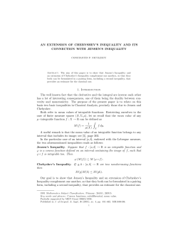
For the two-location model, optimal procurement and transshipment policies for different combinations of Xl and x2 can
be represented as in Figure
2.l~
which shows different regions
for different kinds of optimal policies and the quantities involved.
Region 8 is the "no-action" region; i ..!!", if the in-
itial stock point falls in this region 9 no procurement or
transshipment takes place.
From all other regions the optimal
policy is to reach the boundary of region 8, which is accomplished from each region as follows.
1.
From region I, (Y 19 Y2 ) is reached by ordering Yl-x l
at location 1 and Y2-x2 at location 2.
2
From region 2, (x l ,Y 2 ) is reached by ordering Y2 -X 2
at location 2 only.
0
So
From region 3, (Y l ,x2) is reached by ordering Y1-xl
at location 1 only
0
37
5
y'2J----........:lo-~
8
3
y 21----~-___,=__-_r..
I
I
/
/
I
/
/
I
1
2
y'
1
Figure 2 1
0
4
0
Optimal procurement and transshipment policies
for the single period model
From region 4, (yi'Y2) is reached by transshipping
xl-yi from location 1 to location 2 and then ordering
Yi+Y2-xl-x2 at location 2
0
From region 5, (Y l 'Y2) is reached by transshipping
from location 1 to location 2 and then ordering
50
2
x2-Y
Yl+Y~-Xl-x2 at location 1.
6
0
From region 6,
(xl ,x 2 )
is reached only by trans-
shipping xl-xl from location 1 to location 2, where xl and
x 2 are the solutions of c - DlWl(xl) + Dl W2 (x 2 ) = 0 and
xl + x 2 = k, k being the total initial stock for the whole
system.
38
From region 7~
7.
(x l 'x 2 )
is reached only by transship-
ping X2 -X 2 from location 2 to location l~ where xl and x 2 are
the solution c + DlWl(x l ) - DI W2 (x 2 ) = 0 and xl + x 2 = k.
2.7
Convexity of Optimal Cost When
OsAI,0~2
In Section 2.4, DlWI(Yl,t) and Dl W2 (Y2,t) were shown to
be monotonic nondecreasing continuous functions of Yl and Y2'
respectively.
This property will be used to show that the
optimal cost f(x l ,x ), that is~ the total cost of the whole
2
system following an optimal policy, is a convex function of
Xl and x 2 ' Following Figure 2.1, one can show that f(x l ,x2)
is convex in each region, Section 2.5 shows that when t ~ 0,
WI(YI,t) and W2 (Y2,t) are, in fact, Wl(YI+t) and W2(Y2-t).
For simplicity, Wl(YI+t) and W2(Y2-t) when t ~ 0 and
WI(Yl-ltl) and W2(Y2+lt\) when t
gion 1, xl < Y1 , x 2 < Y2 and
fore,
f(xI'X 2 )
=
t
=
~O
are used here.
0, YI
=
YI , Y2
=
In re-
Y2.
There-
cl(YI-xl) + c 2 (Y 2 - x 2) + W1(Y I ) + W2 (Y 2 )
Dlf(xl,x2) = -cl
D2 f(xl,x2) = -c2
Dilf
= D22 f = Dl2 f = D2l f = 0,
and f(xI,x2) is trivially convex since it is linear in both
xl and x 2 .
In region 2, Yl ~ xl ~ Vi; X2 < Y2 and t = 0, Yl
Y2 = Y2 • Therefore,
=
xl'
39
f(x 1 ,x 2 ) = c 2 (Y2- x 2) + WI(x l )
D1 f(xl,x2) = D1WI(xI)
D2 f(x!,x2)
+
W2 (Y2)
= -c 2
D11f ~ DIIWI(x l ) ~ 0; D22 f = 0; D12f = D2l f
and f(x l ,x 2 ) is convex in xl and x 2 in region 2.
In region 3, xl < YI , Y2 oS. x 2 oS. Y2; t
Y2 = x20 Therefore,
f(x 1 ,x 2 ) = cI(YI-xI)
+
:=
:=
0, Yl
0,
:=
YI ,
WI(Y l ) + W2 (x 2 )
D1f(xl,x2) = -ci
D2 f (xl,x2) = DIW2(x2)
Dllf = 0; D22 f := DIIW2(x~~ 0; D12 f := D21 f := 0,
and f(x 1 ,x 2 ) is convex in Xl and x 2 in region 3.
Yi, x 2 < Y2 , x 1+x 2 S Yi+ Y2; t = xI-Yi,
Yi+Y2- x I" Therefore,
In region 4, Xl
YI = x 1 'Y2
:=
~
f(x l ,x 2 ) = c 2 (Yi+ Y2- X l- x 2) + W1(Yi) + W2 (Y 2 ) + c(xl-Yi)
D1f(xl,x2) = c - c2
D2 f(xI,x2) = -c2
D22 f = Dl2 f = D2l f = 0,
and f(x 1 ,x 2 ) is trivially convex in region 4.
Dllf
~
2'
YI
=
In region 5, Xl < YI , x 2 ~ Y
x I +x 2
Y1+Y2- x 2' Y2 := x 2 " Therefore,
~
Yl+Y
f (Xl ,x ) = c (Yl+Y~-xl-x2) + WI (Y 1) + W2 (Y
2
i
D1f (x 1 ,x 2 ) = -c 1
D2f(xI,x2) = c - ci
e
D11f = D22 f = Dl2 f = D21 f = 0,
and f (xl'x ) is trivially convex in region 5
2
2; t
2)
:=
x 2 -Y
+ c(x -Y
2
2,
2)
40
In region 6, xl+x2 > Yi+Y2 and c
and Y1
=
xl' Y2 = x2' t
When t
~
DIWl(xl) + Dl W2 (x2) <
= t(xI'x 2 )·
= t(X 1 ,X 2 ),
(2.24)
Differentiating (2.24) with respect to xl yields
-DI1W1(x1-t) (1-D1t) + DIIW2(x2+t)Dlt
= o.
therefore,
(2.25)
Differentiating (2.24) with respect to x2 yields
DIlWl(xl-t)D2t + D11W2 (x 2 +t) (I+D 2 t)
= O.
Therefore~
.
•
(2.26)
Since f(x 1 ,x 2 ) = ct + W1(x1-t) + W2(x2+t)~
DI f(x 1 ,x 2 ) = eDIt + D1W1(X1-t) (l-Dlt) + D1W2 (x 2 +t)D 1t
- D1WI (x 1 -t)
because of (2.24), and
D2 f(x 1 ,x 2 )
= cD 2 t ~ D1W1 (x 1-t)D 2 t + Dl W2 (x 2 +t) (1+D 2 t)
= D1W2 (x 2 +t)
because of (2.24).
Thus,
D1If
= D1IWI(XI-t) (l-DIt).
(2.27)
Substituting (2.25) in (2.27) yields
DI1f
= DIIWI(Xl-t)DllW2(x2+t)/[DllWl(xl-t)
~
Thus,
O.
+ DllW2 (X2+ t )]
~
41
(2.28)
Substituting (2.26) into (2.28) yields
D22f ~ DIIW1(xl-t)DllW2(x2+t)/[DllWl(xl-t) + D1IW2 (x2+ t )]
~
o.
and
D12 f
= D21 f
=
D11W 1 (Xl-t)DllW2(X2+t)/[D11Wl (xl-t) + D11W2 (x 2 +t)]
~
o.
Thus it is shown that
Dllf
= D22 f = D12 f
=
D21 f
~
o.
Hence 9 f(x 1 ,x 2 ) is convex in xl and x 2 '
In.region 7, xl+x2 > YI+Y2 and c+ DIW1(xI) - DI W2 (x 2 ) < 0,
and YI
= Xl' Y2
When t
~
=
x2 ' t
= t(xl,x2).
t(Xl'X 2 ),
(2.29)
Differentiating (2,29) with respect to Xl yields
DIIW1(Xl+t)(1+Dlt) + DIIW2(x2-t)Dlt ~
o.
Therefore,
(2.30)
Differentiating (2.29) with respect to x 2 yields
DIIWl(xl+t)D2t - DIIW2 (x 2 -t) (1-D 2 t)
=
o.
Therefore 9
(2.31)
42
Since
f(xl~x2)
= ct
WI(x1+t) + W2 (x 2 -t)9
D1f(Xl'X2) = cDlt + DIW1(XI+t) (1+D1t)
+
= D1W1(XI+t),
because of (2.29) and
D2 f(x 1 ,x 2 ) = cD 2t + D1W1 (x l +t)D 2t + DI W2 (X 2 -t) (1-D 2t)
= D1W2 (x 2 -t)
because of (2.29).
Thus,
(2.32)
SUbstituting (2.30) into (2.32) yields
Dllf = DIIWI(xl+t)DlIW2(X2-t)/[DlIWl(Xl+t) + D1lW2 (x2-t
~
)]
0
and
D22 f = Dl1W2 (X 2-t) (1-D 2t).
Substitut10n of (2.31) in (2.33) yields
(2.33)
D22 f = DllWl(xl+t)DlIW2(x2-t)/[DllWl(xl+t) + D11W2 (x 2-t)] ~
D12 f = D21 f
o.
= DIIWl(xl+t)DllW2(x2-t)/[DllWl(xl+t) + DllW2 (X 2-t)] ~ o.
ThUs, Dilf = D22 f = Dl2 f = D2l f
convex function of xl and x2.
~
O.
Therefore, f(x l ,x 2 ) is a
In region 8, Yl = xl' Y2 = x 2 , t = O.
Therefore,
f(xl,x2) = Wl(xl) + W2 (x2)
= sum of two convex functions.
Therefore, f(x 1 ,x 2 ) is convex in xl and x 2 .
It is proved in Section 2.4 that DIWl(xl) and DlW2(x2)
are monotonic nondecreasing continuous functions of xl and x2'
respectively; hence, Wl(xl) and W2 (x2) are convex functions.
Therefore, for any two points xl and Yl'
43
(2.34)
and for any points x2 and Y2'
(2.35)
Let ~(WpxpY) denote the quantity
W(X) - W(y) - (x-y)D1W(x).
Then the criteria of convexity, (2.34) and (2.35), of WI(xI)
and W2(x2) are equivalent to b(WlpXl,YI) ~ 0 and
~(W2,X2'Y2) ~ O.
These criteria are used to prove the con-
vexity of f(xI,x2)'
First it is shown that Dl f(xl,x2) and
D2f(x l ,x 2 ) are monotonic nondecreasing continuous functions
of xl and x2' respectively.
If xl < YI , x2 < Y2 , then
Dl f(xl,x2)
=
-ci
Lt xI-> 0, Dl f(xl,x2) -?> -cl
If YI ~ xl ~ YI , x 2 < Y2 , then
Dlf (xl ,x2) = DIW I (xl) .
Lt xl
YI , Dl f(x l ,x 2 ) ~ DIWI(Y I ) = -c
,
Lt Xl---i> Yi, Dlf (xl ,x ) ~ DIW (Y i,) = -c > -c ·
1
I
l
2
If yi < xl' x 2 < Y2' and x I +x 2 < Yi+Y2' then
~
=
-c
,
If xI+x2 > Yi+ Y2 and c - DIWI(xl) + D1W2 (x2) < 0, then
Dl f(xl,x2)
= DIWI(xl-t) = DIWI(xI)'
If (x l ,x 2 ) lies in the no-action region p then
Dl f(xl,x2)
Lt xl ~
xl'
=
DIWI(xI)'
DIW I (xl) ~ PIW 1 (Xl) .
a function of two or more arguments is written as
f(X)
~
fey)
+
(X-Y)'Vf(Y)9
or equivalently,
O(f,X,Y) ~
o.
The results hold for any two points in the positive
quadrant of the (x l ,x 2 )-plane.
here,
A few typical cases are shown
When X lies in the no-action region and Y lies in region 1,
f(X)
= W1 (xI)
fey)
=
+
W2 (x2)
cI{YI-YI) + c2(Y 2 -Y2) + W1(Y l ) + W2 (Y 2 )
Dlf (Y)
=
-ci
D 2 f(Y)
= -c 2 '
Therefore,
When X lies in the no-action region and Y lies in region 2 9
f (X) "" WI (xl) + W2 (x2)
f (Y)
=
Dlf (Y)
D2f (Y)
c 2 (Y 2 -Y2) + WI (YI) + W2 (Y 2 )
=
DIWI (YI)
Therefore~
~(f,X,y) = a(Wl'Xl'Yl) + ~(W2,X2'Y2) + c2(Y2-Y2)
~
o.
When X lies in the no-action region and Y lies in region 4,
f(X) = Wl(xl) + W2(x2)
fey) = c2(Yi+Y2-Yl-Y2) + Wl(Yi> + W2 (Y 2 ) + c(Yl-Yi)
Dlf (Y) = c - c2
D2 f (Y) = -c2
Therefore,
b(f ,X,Y) = b(Wl,xl,Yi) + b(W2,x2'Y 2 ) + c2(Yi+Y2-Yl-Y2)
~
0,
since Y1+Y2 < Yi+Y2.
When X lies in the no-action region and Y lies in region 6,
= Wl(xl)
f(X)
+ W2 (X2)
fey) = ct + Wl(Yl-t) + W2(Y2+t)
Dl f (Y) = DlW1 (Yl-t)
D2f(Y) = D2W2 (Y2+t ).
Therefore~
~(f,X,Y) = ~(Wl'Xl'Yl-t) + ~(W2,x2'Y2+t)
- t[c - DlW l (Yl-t) + D2W2 (Y2+ t )]
~
o.
When X lies in region 6 and Y lies in region 1,
f(X)
= ct
+ Wl(xl-t) + W2(X2+ t ) .
fey) = cl(Yl-Yl) + c2(Y2-Y2) + Wl(Yl) + W2(Y2)
46
DIf (Y) :: -c 1
D f (Y) :: -c •
2
2
Therefore~
b(f~X,Y )
= ct + W1(x1-t) + W2 (x 2 +t) - cl(Y1-Yl)
- c2(Y 2 -Y2) - W1(Y 1 ) - W2 (Y 2 ) + cl(x1-Yl)
+ c2(x2-Y2)
:: ~(Wl,xl-t'Yl)
~
+ ~(W2'X2+t~Y2) + t(c+ci- c 2)
o.
When X lies in region 6 and Y lies in region 2,
f(X) = ct+ W1(xl-t) + W2(x2+t)
fey) :: c2(Y 2 -Y2) + W1(Yl) + W2 (Y 2 )
D1f(Y) :: D1Wl(Yl)
D2 f (Y) :: -c 2 ·
Therefore
b(f,X,Y) = ct + Wl(xl-t} + W2 (x 2 +t) - c2(Y 2 -Y2} - W1(Yl}
- W2(Y2) - (xl-Yl}DlWl(Yl) + c2(x2-Y2)
= ~(Wl,xl-t'Yl) + b(W 2 ,x 2 +t,Y 2 )
+ t [c - D1W 1 (Yl) - c 2 ]
~ b(Wl,xl-t'Yl) + b(W 2 ,x 2 +t,Y 2 ) + t(c+ci- C 2)
2: 0
0
When X lies in region 6 and Y lies in region 4,
f(X) = ct + Wl(xl-t) + W2(x2+t}
fey} = c2(Yi+Y2-YI-Y2} + W1(Yi) + W2 (Y 2 ) + c(YI-Yi}
D1f(Y) = c - c2
D2 f(Y) = -c2°
47
Therefore,
~(f,X,Y) :: ct + Wl(Xl-t) + W2 (x2+ t ) - C2(Yi+Y2-Yl-Y2)
+ Wl(Yi) - W2 (Y 2 ) - C(Yl-yi) - (C-c2)(xl-Yl)
+ c2(x2-Y2)
:: Wl(xl-t) - Wl(Yi)
(C-c 2 ) (x I-t-Y i)
+ W2 (x2+ t ) - W2 (Y 2 ) + C2 (x2+ t - Y2)
~
O.
When X lies in region 7 and Y lies in the no-action region,
f(X) :: ct + Wl(Xl+t) + W2(x2-t)
fey) :: Wl(Yl)
Dlf (Y)
.
=
+
W2 (Y2)
DlW l (Yl)
D2 f(Y) :: Dl W2 (Y2)'
Therefore,
b(f,X,Y)
= ct + Wl(xl+t) + W2 (x2- t ) - Wl(Yl) - W2 (Y2)
- (xl-Yl)DlWl(Yl) - (x2-Y2)D l W2 (Y2)
:: ~(Wl,xl+t'Yl)
+
~(W2,x2-t'Y2)
+ t [c + DlW l (Yl) - D2W2 (Y2)]
~
o.
It has been proved that f(xl,x2) is convex over region
6 and the no-action region and also over region 7 and the noaction region.
To prove that f(xl,x2) is convex over all
three regions, let X and Y denote two points in region 7 and
region 6, respectively. Let Yl and Y2 be two points in the noaction region, on the line joining X and Y.
point on this line outside interval (Y l ,Y 2 ).
Let Z be any
Suppose Z lies
48
between Y2 and Y; then Y1 , Y2 , and Z can be written as
.
(2.36)
(2.37)
(2.38)
and also
Z
=
~OX
t
t
Ai+~i=l,
+ AOY'
i=0,1,2,3.
(2.39)
Now substituting (2.36) into (2.37),
e
Y2 =
1
t
~IX2
-
t
A2 A1
X +
A2
1 -
A2A~
Z.
(2.40)
Substituting (2.40) in (2.38),
Z =
Since Yl , Y2 ,·and Z all lie on the line joining X and Y,
gion,
Also, since f(xl,x2) is convex over region 6 and the no-action
region,
and
feZ)
~
A3 f(Y 2 ) +
t
~3f(Y).
It is observed that 1-X2Xi and 1-A2Ai-A3~2 are both positive
.
49
numbers.
Therefore, by substitution of fCY l ) and f(Y2) ,
feZ) ~ AOf(X) + XOf(Y).
,
But Z = XoX + ~OY.
Therefore,
f(~oX+~OY) ~ AOf(X) + AOf(Y).
Hence, f(xl,x2) is convex over regions 6 and 7 and the noaction region.
This concludes that
f(xl,x2) is convex everywhere in the
positive quadrant of the (xl,x 2 )-plane.
It is noted that when 0 ~ Aj , Wj(Xj) (j=1,2) is conTherefore, f(x l ,x 2 ) is convex over the whole positive quadrant of the (x l ,x 2 )-plane.
tinuously twice differentiable.
But, in other cases, Dl1Wj(X j ) does not exist everywhere.
Therefore, f(xl,x2) is at least sectionally convex.
~e
50
3
0
THREE-LOCATION SINGLE=PERIOD MODEL
In Chapter 2 the optimum inventory policy of the twolocation problem for a single period was discussed in great
detail.
In this chapter, a spatial generalization of the
two-location problem is considered.
Here it is assumed that
there are n-locations under a centralized multilocation system.
Each location can procure any amount it needs from a
central warehouse and also can transship a certain amount of
its surplus stock to any other location.
However, it is as-
sumed that it is not advantageous for a location to receive
as well as transship.
In other words, if cii denotes the
cost of procuring one unit of an item from the central warehouse to location i, and if Cij denotes the cost of transshipping one unit of the same item from location i to location j,
.
then it is assumed that c ii + c ij > Cjj and Cij + Cjk > cikThe first inequality says that it is cheaper to order a unit
to location j directly from the central warehouse than to
procure it at location i and then transship it to location j.
The second inequality says that it is cheaper to transship a
unit directly from location i to location k than to send it
via location j.
3.1
n-Location Mode1--Its Procurement
and Sale Policy
The cost function of the n-location problem for a single
period is written in most general form and the optimum special sale policy and procurement policy are derived for fixed
-_
51
transshipment.
For the analytical complexities, the optimum
transshipment policies are derived only for the threelocation problem.
The notations used in Chapter 2 are gen-
eralized for n-locations,
In addition, the following new no-
tations are introduced,
ci1
= cost of procuring a unit of an item from the central warehouse to location i,
c ij
=
cost of transshipping a unit of an item from location i to location j (cij
t ii
:-
=
Cj i'
i
,. j).
amount procured at location i from the central
warehouse (Yi
t ij
::
=
xi + t ii ) ,
amount transshipped from location i to location j
(t ij
~ 0;
i ,. j).
It is observed that the cost function of the n-Iocation
problem becomes completely separable except for the transshipment cost,
Lx(Y,X,T)
The cost function is
52
(3.1)
Let zi(Yi~Ti) denote the optimal special sale policy
when procurement level Yi at location i and transshipment
quantities tijis are fixed.
Then as in the two-location
problem, the structure of zi(Yi,'ri) is given by theorem 3.1.
The proof of the theorem is exactly similar as in the twolocation problem.
Theorem
Therefore, the proof is omitted here.
3.l~
If Pi
~
qi
~
0 and
if 0 ~ Ai, then zi(Yi~Ti) ~ O.
i.
ii.
if Bi
~ O~
then zi(Yi,Ti)
Yi + '1"1
if Ai < 0 < B i , then there exists a unique posi-
iii.
tive number Zi, ai < Zi <:
Z i (y i ~ Ti)
=:
= O~
for (Z 1 /q i)
-
-
=~
such that
T1 <: Yi < =
qi (y i +'r i)
for (Z i/Pi) - 'fi ~ Yi ~ (Zi/qi)-'l"i
qi
Pi
=:
'fi
Yi + 'l" i ~ for 0 oS Yi < (Z i/pi)
This theorem gives 3 n different special sale policies.
=
Zi
-
-
It is observed that (3.1) can be written as
Lx(Y~Z~T)
n
=:
L: [cii(Yi-xi)
i=1
+
gi(Yi~zi~Ti)]
+
2: ciJ·tiJ"
irj
(3.2)
53
Substituting zi(Yi9 T1) for zi in gi(Yi9Zi,Ti) and calling the
nes function Wi (Yi 9T i)' it can be proved as in the twolocation problem that Wi(Yi,Ti) is a convex function of Yi.
Moreover, Wi(Yi,T i ) is of the form Wi(Yi+Ti). Henceforth,
Wi(Yi,T i ) is written as Wi(Yi+Ti).
It is noted that
DIWi(Yi+'I"i) = Dlgi[Yi,zi(Yi+ 'l"i,'I"i J
+ D2 g i [Yizi(Yi+ Ti) ,'I"iJ [dzi(Yi+Ti)/dYiJ
Yi+ Ti-zi
Dl g i (Yi,zi,'1'i) =
*
(hi - (ri+si)Pi
a
(3.3)
S
i
+ (r i+ s i)P i 0 i [P i (Y i+'I" i) - (Pi-qi) CrlJ¢r(Cr)dCr
+ (-r i - siqi + (r i +s i )qi0 i[qi(Yi+'T'i)
+ (Pi-qi)ziJ } [1 - 0r(Yi+'1'i-zi)]
(3.4)
*
D g . (y . ,z . , '1" .) = V. [q. (Y . + T .) + (p. -q .) Z .l [1 - 0. (y . + '1" • -z .)] ,
1.
1.
1.
1.
1.
1.
1.
1.
1.
1.
1
2 1. 1. 1. 1.
(3.5)
where Vi(9i) = Ai + (ri+si) (Pi-qi)0i(9i)·
Let the parametric structures cii+hi+ h i - (ri+si)Pi and
cii+h!-r!-siqi be represented by Mi and Ni , respectively.
Let Yi i denote a number such that
c i i + D1Wi (Y ii' 0) = O.
Theorem 3.2:
and if 'l"i
'1".
~
1. ~
If Ai < 0 < B i , Ni<O,xi
~
Yii , i=1,2,···,n,
0 and xi+'T'i > Yib then Yi ('I" i) = xi
.. -'1'.
0 and xi+'T'i < Yii' then Yi ('I" i) = Y11
1
'l"i < 0,
then Yi (T i) = Yii+I'I"il.
54
Proof~
If Ai < 0 < Bi from (3 3)9 (3.4)9 and (3.5),
0
+,. .)
DlW.1. (y 1.. 1.
Therefore,
:; h! - rt - siqi + (l1" i+ s i)Qi 9J i [Cl i (y i+'f i)] .
cii + D1Wi(O,O) = Ni ,
and if Ni < O'Y ii > 00
Now the total cost of the n-location problem following
an optimal special sale policy for a given set of values of
YIY2o.oYn and Tl T2 o.oT n , where Yi
n
L (Y , T) =
Z C .. (y . -x .)
. 1 11. 1. 1
1=
+
~
Ti ~
Xi and
° is
n
~ W. (Y . + 'I" .) + ~ c· . t ..
. 1 1.
1.
1.
. oJ' l.J l.J
1=
(3.6)
°
l.'J
Differentiating (3 6) with respect to Yi yields
0
DiL(Y,T) = cii + DIWi(Yi+Ti)·
Now if Yi + T i <
Y ii 9
and if Y i + T i > Y ii'
Cit + DlWi(Yi+Ti) > 00
Since Yi
~
= Y.1.1.
.. -,...1
2: xl.' such that
Xi' when Xi +
Ti ~
Yii , there exists a Yi
(1
i)
cl.'1.' + DlW.[y,('f,)+T.]
= 0,
1.
1.
1.
1.
and since Wi(Yi+'f i ) is a convex function of Yi' Yii-T i must
be optimal for Yi ,
If xi+Ti > Vii' then any additional procurement from the
central warehouse only increases the cost, and since
Wi(Yi+Ti) is a convex function, 1i(r i ) = xio
If r i < 0, differentiating (3.6) with respect to Yi
yields
55
Since xi < Yii , there exists a value
Yi ('I' i) = Y1i + I 'f i
I
> Yii > xi
such that
c ii + D1Wi[Yi('l'i) - l'I'i\J = 0,
and since Wi(Yi+Ti) is a convex function of Yi' Yii+ITil must
be optimal for Yi y which proves the theorem.
Theorem 3.3:
i and xi > Yii and if 'f i
then Y.1. ('T 1..) = x·'
and if 'T.1<: .O.' then Y'1. ('I' l..) = X1.' when
1.'
X
i-I 'I" i
I
~
<: 0 < B
~ Y ii am Yi ('T i) :; Y1i+ I'T i
Proof:
3.2.
If Ai
I
when x i-I 'I" i
I
0,
< Yii·
The proof has similar reasoning as in theorem
Here the conditions N i
<: 0
are not needed.
In theorem
3.2 these conditions ensured nonnegative Yiiy whereas the
present theorem holds for negative Yii as well.
Differentiating (3.6) with respect to Yi yields
DiL(Y p T)
Since xi > Yiiy for Yi
~
==
c ii + D1W i (y i+'I" i) .
x iy
cii + D 1Wi (Yi+'I"i)
~
Oy
and since Wi (Y i +'I"i) is a convex function y Yi('I'i) = xi.
If
'l'i < Oy
DiL(Yy'T) = cii + DlWi(Yi-ITil).
If xi-ITil ~ Yiiy wbenever Yi > x iy Yi-I'fil ~ Yii .
Therefore,
cii + D1Wi(Yi-I'Til> ~ 0,
and since Wi(Yi+'I"i) is a convex function y Yi('Ti) = xi-
But,
if Xi-ITil < Yiiy for Yi > xi there exists a Yi(Ti) = Yii+\Til
such that
56
and since Wi(Yi+Ti> is a conve~ fu~ction of Yi 9 Yii+!Til must
be optimal for Y1 9 which proves the theorem,
3.2
Triangle Restriction and Characterization
of Optimal Transshipment Policy
For discussing the procedure of deriving optimal transshipment policy it is assumed that the whole system has only
three locations,
In a three-location procurement problem,
there are four different situations:
i.
Three stores order,
ii.
Two stores order,
iii.
One store orders,
iv.
No store orders,
For each of these situations typical
shipment policies are considered;
cas~s
of optimal trans-
In Chapter 2 a lemma was
introduced which proved that under a triangle restriction
of procurement and transshipment cost it is not economical
both to order from the central warehouse and tranship simultaneously at a location.
The lemma is applicable in the
three-location problem as well.
In addition 9 another lemma
is introduced here to prove that under the triangle restriction of transshipment costs it does not pay to receive and
transship from the same location,
Lemma
If c .1J
.. +c'k
> c;k and if t .. > O. then
J ~
J1'
t kj = 0 for every i,j9k = 1,2 93 and 1 ~ j ~ k,
3,1~
.. _
57
Since the transshipment quantities are nonnega-
Proof~
.
tive 9 then» if possible 9 let t kj > O. Now there are two
cases to cons ider, t kj > t j i and t kj < t j i'
If t kj
~
t ji9 then as an alternative, location j can re-
ceive and amount tkj-t ji from location k 9 and location i can
receive an amount t ki which is qual to t ji from location k 9
and location j transshipping nothing to location i. Under
this new transshipment plan, all other costs remain the same,
So the difference in cost between the two policy decisions is
the difference between the cost of two ways of transshipment.
J
Expected cost for _ Expected cost for
[ original policy
alternative policy
= c kj t kj
~
+ c j it j i
Ckj t kj + c j it j i
- c kj (t kj -t j i)
Ckj (t kj -t j i) - ck·1.t J..1.
:: (Ckj+C j i-cki) t j i
~
If
O.
t kj <
tji~ then, as an alternative 9 location i can
receive an amount tji-t kj from location j and an amount t ki ,
which is equal to t kj » from location k; and location j re
ceiving no transshipment. In this case,
Expected cost for _Expected cost for ]
[ original policy
alternative policy
=
ckjt kj + cjit ji - c ji (tji-t kj ) - ckit ki
"" c kj t kj + c j it j i - c j it j i + c j i t kj - c k i t kj
= (Ckj+Cji-Cki)tkj
~
0,
which proves the lemma.
58
It is noted that the first situation when all the three
stores order is not of much
since in this case by
interest~
lemma 3.1 t .. = 0 for all i and
J.J
j~
~
i
j.
This is the case
of three stores adopting their optimal procurement and special
sale policies independently.
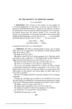
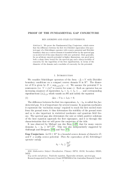
of ordering and transshipment.
Figure 3.1 shows typical cases
The center of a triangle
represents the central warehouse and the veritices represent
the three stores.
The arrow indicates the direction of or-
dering and transshipment.
3
1~
g
3
2
1
2
Three stores
order
...
3
&
2
1A2 1B
2
Two stores order
3
1
3
3
1
&
3
3
2
1L1 L1
2
1
2
One store orders
3
16
3
3
2
1
6
2
1
62 16
No store orders
"_
Figure 3.1
3
Typical cases of optimal ordering
and transshipment
2
-e
59
3,3
Description of Optimal Transshipment
and Procurement Policies
In Section 3.2 a number Yii was defined to satisfy
= O.
cii + DIWi(Y ii )
to satisfy
Here, another number 9 Yij , is defined
c ji + DlWi(Y ij ) = 0 9 i f j9 (cij=C ji ) , and
because of triangle restriction of ordering and transshipment
cost 9 Yii
C
~
jj
-
Yij ,
critical number,
The number Y ij may be called
transshippin~
The position of xi relative to Yij deter-
mines whether or not it is permissible to transship from 10cation i to location j,
X. > Y"
1.
l.J
9
At a particular situation, if
it may be profitable to transship from location i
to location j, but if xi < Yik , it is not profitable to transship from location i to location k,
Let Aij <9 l ,9 2 ) denote the marginal cost of transshipment
from location i to location j, when the levels to stock are
9 1 and 9 29 respectively.
Then,
Aij (9 l ,9 2 ) = c ij - DI Wi (9 l ) + Dl Wj (9 2 )·
Let Aii(9) denote the marginal cost when location i with stock
level 9 procures from the central warehouse.
Aii (9)
Clearly Aii(Y ii )
=
O.
=
Then 9
Cii + DI Wi (9).
The typical cases of transshipment and
procurement are described below with reference to Figure 3.2,
1.
Three stores order:
If xl < Y1I , x 2 < Y22 , x 3 < Y33 ,
the point Yll'Y22'Y 33 is reached by ordering Y11-X 1 at location 1, Y22 -x 2 at location 2, and Y33 -x 3 at location 3,
.'
e
e
1
I
2
YII
1
2
YII
A
Figure 3.2
~
e
3
3
3
"
2
Y33
B
c
Regions of optimal procurement and transshipment policies
0')
o
"
.. _
61
2.
Two stores order:
i.
xl < Yll~ x 2 < Y22~ and
Y33 < x 3 <: min(Y31~Y32)'
An amount YII-X I is procured at location l~ Y -x is procured
22 2
at location 2, and nothing is procured at location 3.
iia.
xl < Y1I , x 2 < Y22' Y33 < Y31 < x 3 < Y32 , and
xl+X3 <: Y11+Y31 .
Since x3 >
Y31~
to location 1.
it is permissible to transship from location 3
An amount x3-Y31 is transshipped from location
3 to location 1, Yll+Y31-xl-x3 is procured at location 1, and
Y -x is procured at location 2 from the central warehouse.
22 2
iib. xl < YII~ x 2 < Y22~ Y33 <: Y32 < x 3 <: Y31 , and
X 2 +X S <:
Y32+ Y22'
Since x
> Y , it is permissible to transship from location 3
32
3
to location 2. An amount x3-Y32 is transshipped from location
3 to location 2, Y32+Y22=x2-x3 is procured at location 2,
~nd
Yll-x l is procured at location I from the central warehouse.
xl < Yl1; x 2 < Y22 ; x 3 > Y32 > Y31 > Y33 ;
x +x < Y +Y ; and x +x < Y +Y .
1 3
l1 3l
2 3
32 22
The marginal cost of transshipment from x3 to x2 is
iii.
A32(x3~x2)
= c32 - Dl W3 (x3) + Dl W2 (x2)
< c32 - D1W3 (Y 32 ) + Dl W2 (Y 22 )
= c 32 - (c 32 -c 22 ) - c 22
= O.
62
The marginal cost of transshipment from x 3 to xl is
A. 31 (x 3 ~ xl)
= c 31 - DIW3 (x 3) + D1WI (x I)
< c S1 - DlWS(Y S1 ) + D1WI(Y lI )
=
Therefore~
xl'
c 31 -
(CSI-C II ) - ell
it is feasible to transship from x3 to both x 2 and
Suppose t 32 > O~ t Sl > O~ tIl > O~ and t 22 > 0 constitute
the optimal policy.
The total cost under this policy is
cllt 1l + c 22 t 22 + cSlt Sl + c 32 t S2 + Wl(Xl+tll+tSl)
+ W2(X2+t22+t32) + W3(x3-t32-t3l)'
t* = t
32
32
Let
t;l =
t 3l
til = tIl
-
I::.
+ I::.
-
6
+ 6
t* :: t
22
22
denote an alternative policy where I::.
positive number,
(3.7)
is an inf inites imal
It is then observed that
* + t* = t
+ tIl
tIl
31
3l
t;2 + t;2
=
t
22
+ t
32
+ t
t* + t* = t
31
32
32
3l ·
The total cost under this alternative plan is
c
t* + C t* + C t* + C t* + W (x +t +t )
11 11
22 22
31 31
32 32
1 1 11 31
+ W2(x2+t22+t32) + W3(x3-t32-tSl)'
(3,8)
Subtracting (3.8) from (3.7) yields
(3.9)
63
Now since Y32 > Y31Y D1WS (Y 32 ' > D1WS (Y S1 '
or
(c32- c 22) > (cS1-c1l)'
31 ~cll)J :> O.
This means the total cost can be reduced by decreasing t 32 to
zero. The optimal policy is: x -Y
is transshipped from
3 31
location 3 to location 1, Yll+Y31-xl-x3 is procured at locaTherefore Y
t::. [(c 32 -c 22 ) -
(c
tion 1, and Y -x is procured at location 2.
22 2
3. One store orders:
i.
xl <: YII ; Y
<: x <: min(Y
,Y );
21 23
22
2
Y33 < x3 < min(Y 31 ,Y 32 )·
Now, with reference to A, Figure 3.2, (x l ,x 2 ) lies in region
3; in B, Figure 3,2, (x l ,x3) lies in region 2; and in C,
Figure 3.2, (x 2 ,x 3 ) lies in the no-action region. Therefore,
the optimal policy is just to procure Y11-x l at location I
from the central warehouse.
Xl <: YII ; Y22 < Y21 < x 2 < Y23 ;
x 1 +x <: YI1 +Y 21 ; Y33 < x 3 <: min(Y 31 ,Y 32 )·
2
In C, Figure 3.2, (x 2 ,x 3 ) lies in the no-action region. The
ii.
optimal policy is to transship x2-Y21 from location 2 to
location I and procure YII+Y21-xl-x2 at location I from the
central warehouse,
iii.
Xl <: YI1 ; Y22 < Y21 < x 2 < Y23 ;
Y33 < Y31 < x 3 < Y32 ; and
x I +x 2 +x 3 <: YII+Y21+Y31·
In C, Figure 3,2, (x2,x3) lies in the no-action region.
The
optimal policy is to transship x2-Y21 from location 2 to location 1; transship x3-Y31 from location 3 to location 1; and
--
64
then order
YIl+Y21+Y31-xl-X2~X3 to
location 1 from the cen-
tral warehouse.
4.
No store orders:
YII < Xl < min(Y12'Y13); Y22 < x 2 < min(Y 21 ,Y 23 );
and Y33 < x3 < min(Y 31 ,Y 32 ).
The point is already in equilibrium and lies in the no-action
region in A, B, and C, figure 3.2.
Therefore, neither trans-
shipment nor procurement is done.
In Figure 3.2, the (x.,x.)-plane is divided into eight
1
regions.
J
Regions I through 5 have already been described.
In order to describe the cases in regions 6 through 8, the
following notations are introduced to prove a few lemmas in
this section.
The relevant theorems of optimal transshipment
policies are presented in Section 3.4.
Let Rij , Rji , and Rij denote the set of points (Xi,X j )
such that
if (Xi,X j )
E Rij , then Aij(Xi,x j
)
< 0 and
xi+Xj > Yij+Y j j .
if (xi,x j )
E Rji , then Aji (Xj,xi) < 0 and
xi+x j > Yji+Y ii ·
if (Xi'X j ) E Rij' then both Aij(Xi,Xj) and Aji(Xj,x i ) ~ O.
In a three-location problem there are three pairs of
marginal cost expressions:
AI2(xI,x2),A21(X2,xl);
A2S(x2,xS),A32(x3,x2); and AI3(xl,x3),ASl(x3,xl).
These quan-
tities satisfy certain sign and magnitude restrictions which
are proved in forms of the following lemmas.
--
65
If Aij{Xi,x j ) < 0, then Aji(Xj,x i ) >
Lemma 3.2:
Proof:
o.
Since Aij{Xi,Xj) < 0, DlWi(xi) > Cij+D1Wj(Xj)
).,ji{Xj,xi) = cji - DlWj{x j ) + DlWi{xi)
D1W j (x .) +
::> C •• -
J
J
~
C ••
~J
+ DlW. (x .)
J
J
= 2c ij , since c ij = c ji
>
Lemma 3.3:
o.
If Aik(xi,xk) = Aij{Xi,Xj), then
A. jk (xj,X k ) ~o.
Proof:
From the triangle restriction on transshipment
cost, cik-c ij < c jk ' i f j f k.
Ajk{xj,xk ) = cjk - DlWj{x j ) + DlWk(xk )
~
cik - Cij - DlWj{xj) + D1Wk{xk)
= cik - DlWi{xi) + DlWk{xk)
- [cij-DlWi{x i ) + D1Wj{Xj)].
= Aik{xi,xk) - Aij(xi'X j
)
= o.
Lemma 3.4:
(Xj,X k )
e
If (xi,Xj) E Rij , (xi,x k ) E Rlk' and
Rjk' then Aij{Xi,x j ) reaches zero before Ajk(Xj,xk)
or Aki (xk,xi).
Proof:
If possible, let Ajk(Xj,X k ) become negative before Aij{xi,x j ) reaches zero at a point (Xi,X j ). Then
Aij(Xi,Xj) + Ajk{Xj,xk) must be <0.
But since Cij+Cjk > cik
and DlW i (xi) S DlW i (xi) ,
0_
Aij <Xi,x j ) + Ajk{X j ,x k ) = c ij + cjk - DlW i (xi) + D1Wk{x k )
~ c ik - DlWi(x i ) + DlWk(xk )
= Aik;{Xi,Xk)
~
0, since (xi,xk) ERik.
66
Therefore, Ajk(Xj'X k )
i
0 if Aij(xi,x j ) < O.
Similarly, if
possible, let Aki(xk,xi) become negative before Aij(xi,Xj)
reaches zero at point (Xi,Xj)'
must be <0.
Then, Aki (xk ,xi) + Aij (Xi'X'j)
But, since cki+cij > Ckj and D1Wj (Xj) > DlWj(Xj),
Aki(xk,xi) + Aij(xi,Xj)
~
Therefore, Aki(xk,xi)
=
cki + Cij - DlWk(xk) + D1Wj (xj)
~
Ckj - D1Wk (x k ) + DlWj(x j )
=
Akj (xk ,x j )
~
0, since (xj,x k ) E Rjk
0 if Aij(xi,Xj) <: 0, which proves the
lemma.
If (Xi'X j ) E Rij , (Xj,X k ) E Rkj , and
(xi,x k ) E Rki , then initially transshipment takes place from
location k to location j, and if for any tkj > 0,
Lemma 3.5:
i.
Aki(Xk-tkj'Xi) = 0 and
Aki(Xk-tkj'X i ) > Akj (Xk-tkj,xj+t kj ), then
Aji(Xj+tkj,xi) ~ O.
ii.
Aij(Xi,Xj+tkj)
= 0 and
Aij(Xi,Xj+t kj ) > Akj(Xk-tkj,Xj+t kj ), then
Aik(xi,Xk-tkj) ~ O.
Proof:
The proof is exactly similar in both cases.
Therefore, only one is given.
x ij (x i'X j )
:::
x ki (X k ,xi)
=
Xkj(Xk'X j )
=
Since Ckj <: Cij+cki'
From the condition of the lemma,
c ij - D1Wi (x i ) + D1Wj (x j ) <: 0
- D W (X ) + DlW i (xi) <: 0
c
ki
1 k k
c kj - D1Wk (xk ) + D1Wj (Xj) < O.
\
Akj(Xk,Xj) <: Aij (Xi,Xj) + Aki (Xk,xi) .
67
Therefore~ ~kj(Xk~Xj)
Now~
<0.
has highest absolute magnitude and is
if possible, let
~ji(Xj~xi)
become negative when
~ki(xk~xi) reaches zero and ~kj(Xk~Xj) < 0 at a point
xk
=
xk-t kj and x j
xj+t kj for some t kj > O.
=
IAkj(Xk~Xj) I > IAki(xk,x i )
I,
Therefore,
Akj(Xk,x j ) < 0, and
~ki(xk~xi) = 0; and hence,
Aki(Xk,x i ) - Akj(Xk,x j ) ~ O.
But
).ji(Xj,x i )
=
c ji - DlWj(x j ) + D 1W1 (x i )
~ cki - Ckj - D1W j (Xj)
=
+ Dl W1 (xi)
c ki - DlWk(xk ) + DlWi(x i )
- [Ckj - DlWk(xk ) + D1W j (X j )]
=
~k i (xk ' xi) - ~kj (xk ' x j )
~ O.
Lemma 3.6:
If (Xi'x j ) E Rij ; (xj,xk ) E Rkj , and
(xi,xk) E Rki , then Aji(Xj'Xi) and Aik(xi,xk) both cannot become negative before Akj(Xk,Xj) reaches zero.
Proof:
If possible~ let Aji(Xj,Xi) and ~ik(xi,xk) both
become negative before
(xk ,x j).
Akj(xk~Xj)
reaches zero at a point
Then, Akj (xk' x j ) <: 0
and
~ji (X j ,xi) + ~ik(Xi,xk)
But
Aji(Xj,x i ) + ~ik(Xi'xk)
< O.
"" c ji + c ik - DlWj(x j ) + D1Wk(xk )
> c jk - DlWj(X j ) + D1Wk(xk ,
"" Ajk (X j ,x k )
> 0,
since Akj(xk'x j ) < 0,
68
which is a contradiction,
~ik(xi9xk)
Therefore»
~ji(Xj~xi)
both cannot become negative before
and
Akj(Xk~Xj)
reaches zero,
3,4
Theorems Giving Optimal Transshipment
and Procurement Policies
In Section 3,3 9 the optimal procurement and transshipment policies were discussed for different realizations of
Xl ,X 2 ,x 3 , Here, a lemma is presented first to prove the optimality of the cost function, and then with the help of this
lemma a few theorems are proved for typical situations of
x l ,x 2 ,x 3 to show that the procurement and transshipment policies discussed earlier are optimal.
Lemma 3.7:
If g(X) is a real convex differentiable func-
tion of X (x l x 2 ··,xp ) in a p-dimensional Euclidean space with
xi ~ 0, and if
i.
then
Dig(Xo ) ~
p
° and
ii.
i~XioDi(Xo) = 0,
g(X~
is minimum,
Proof:
Since g(X) is a real convex differentiable func-
tion it can be written as
g(X)
~
g(X o ) +
~ (Xi-Xio)Dig (X o )
i=l
p
L; x iDig (X o ) =
i=l
p
i~XiDig(Xo) .
Now 9 since xi 2:
° and Dig(Xo )
~ 0, then
P
L:xiDig(Xo) ~ 0,
1=1
69
Therefore,
which proves the lemma,
If xl < Y ll , x2 < Y22 , and x3 < Y33 , then
Theorem 3.1:
t ij =
0 for all i,j
=
1,2,3, i "I j, and t ii
=
Yii-xi' i
= 1,2,3.
The proof follows in a similar way as in theorem 2.6.
The total cost is written as
3
g(tll,t22,t33)
=
~ [c .. t .. +
i=l 11 11
w.1 (x 1.+t 11
.. n,
which is a convex differentiable function of tIl' t 22 , and
t 33 ·
Dig(tl1,t22,t33)
If t ii
=
~ii{xi+tii)'
i=1,2,3.
= Yii-xi' then
Theorem 3.2:
If Xl < Yl1' x 2 < Y22' Y33 < Y31 < x 3 < Y32 ,
and xl+x3 < Y ll +Y 3l , then t 31
= x3-Y3l' tIl = Yll+Y3l-xl-x3'
t 22 "" Y22 - x 2'
Proof:
From the definition
By lemma 3.1,
Tl
can be either
t
1 "" t 21 + t 3l - (t 12 +t 13 ).
2l +t 3l or -(t 12 +t I3 ). Now if
T
= -(t 12 +t 13 ), then by theorem 3.2, Yl(11 ) = Yll+t12+t13'
which violates lemma 2.1. Therefore, T1 = t 21 +t 31 , T2 = -t 21 ,
'f
l
and
13 =
Y2{T2 )
t 2l
=
-t 31 .
Again, if
= Y22 +t 21 ,
O.
T2 =
-t 2l , by theorem 3.2,
which violates lemma 2.1.
From the consideration of
1
Therefore,
2 , t 32 can be
~
O.
But
70
since x 3 < YS2 ' t S2
TS
::;
::;
O.
Therefore, '1'1
::;
t SI ' "2
::;
0, and
-t 31 ·
Now, since '1'3 <: 0, by lemma 2.1, Y3
::;
x 3 ' the total cost
can be written as
g(tll,t22,t31) ::; cl1t ll + c 22 t 22 + cSlt SI
+ WI(xl+tll+t31) + W2 (x 2 +t 22 ) + W3 (x 3 -t 3l ),
which is a convex differentiable function of tll,t22,t3l'
Dlg(T) ::; ~ll(xl+tll+tSI)
D2g(T) ::; A22(x2+t22)
D3 g(T) ::; A3l(xS-tSl,xl+tll+tSI)'
If
tIl::; Yll + YS1 - xl - x 3
t 22 ::; Y22 - x 2
t 31
=
x 3 - Y31'
then
Dlg(T) ::; All (Y 11)
D g(T) ::; "-22 (Y22)
2
::;
0
::;
0
Dsg(T) ::; A (Y ' Y 11)
SI Sl
::;
o.
and hence,
tlIDIg(T) + t 22 D2 g(T) + t 31DSg(T) ::; O.
Therefore, by lemma 3.7, g(tll,t22,t3l) is minimum when
tIl::; YII + YSI - xl t 22 ::; Y22 - x
2
Xs
t 3l ::; x3 - Y SI '
Theorem S.S:
If xl <: YII , x 2 < Y22 , Y3S < YS2 < Xs < Y31 ,
and X2 +X S < YS2 +Y 22 , then tIl::; Yl1 -x l , t 22 ::; YS2+Y22-x2-xS'
and t S2 ::; xS-Y 32 .
71
The proof follows exactly in a similar way as in theorem
3.2.
The total cost can be written as
g(tll,t22,t32) :: c11t ll + c 22 t 22 + c S2 t 32
+ W1 (xl+t ll ) + W2(x2+t22+t32) + W3 (x 3 -t 32 ),
which is a convex differentiable function of tll,t22,t32'
Dlg(T) :: All(xl+t ll )
D2 g(T) :: A22(x2+t22+t32)
D3 g(T)
If
=
A32(x-t 32 ,x2+ t 22+ t S2)·
tIl :: Y1l - xl
t 22 =: Y32 + Y22 - x2 - x3
t 32 = x3 - Y32 ,
then
Dlg(T)
D g(T)
2
D3 g(T)
0
=
All (Y 11)
::
A22 (Y22) :: 0
)..32 (Y 32 ,Y 22 )
=
=:
=:
0,
and hence
tllDlg(T) + t 22D2 g(T) + t 32D3 g(T)
=:
O.
Therefore, by lemma 3.7, g(tll,t22,t32) is minimum when
tIl:: Y11 - xl
t 22 :: YS2 + Y22 - x2 - x3
t 32
=:
x3 -
Y 230
If xl < Y1l , x 2 < Y22 , Y33 < Y3l < Y32 < x 3 '
and x +x < Y +Y , x +x < Y +Y , then,
1 3
ll 3l
32 22
2 3
xl - x 3
tIl =: Y11 + Y31
:: Y
x
t
22
2
22
t 3l =: x 3 - Y3l
Theorem 3.4:
-
e
-
t 32
=:
O.
~e
72
Proof:
The total cost can be written as
g(tll,t22,t31,tS2) = cllt ll + c22 t 22 + cS 1 t Sl + c32 t 32
+ Wl(xl+tll+tSl) + W2(x2+t22+tS2)
+ W3(x3-t3l-t32)'
which is a convex differentiable function of tll,t22,t3l,t32.
Dlg(T) = ~11(xl+tll+t31)
D2 g(T) =
=
D3 g(T)
~22(x2+t22+t32)
~3l(x3-tSl-t32,xl+tll+t31)
D4 g(T) = ~32(x3-t31-t32,x2+t22+t32)
If
tIl = Yll + Y31 - xl - x3
t 22 = Y22 - x 2
t 31
~
x 3 - Y31
t 32 ;; 0
.
0
then
DIg (T) = ).,11 (Y 11) = 0
..
D2 g(T) = ).,22 (Y 22) = 0
D3 g(T) = ).,31 (YS1,Y II ) = 0
D4 g(T) = ).,32 (Y 31' Y22) > ~S2(Y32'Y22) = 0
and hence,
tl1Dlg(T) + t 22D2 g(T) + t S1D3 g(T) + t 32D4 g(T) = O.
Therefore, by lemma 3.7, g(tll,t22,t31,t32) is minimum when
tIl = Y1l + YSI - Xl - Xs
t 22 = Y 22 - x2
.
t 3l
It
= x 3 - YSI
t 32 =
o.
73
If xl < Y1I ; Y22 < x 2 < min(Y2l'Y 23 );
Theorem 3.5:
.
Y3S < Xs < min(YSI'YS2), then tIl = Y11-x I , t 21 = t Sl = O.
Proof: The proof has the same reasoning as in theorem
2,7,
The total cost can be written as
g(tll,t22,t31) = c l1 t ll + c2l t 21 + cSlt 31
+ W1(x1+tll+t21+tSI) + W2 (x 2-t 21 )
+ WS(xs-t SI )'
which is a convex differentiable function of tll,t21,t31'
D1g(T) = AII(xl+tll+t21+tSI)
D2 g(T) = A21(x2-t21,xI+tll+t21+t31)
D3 g(T) = ASI(xS-t31,xI+tll+t21+t31)
If
tIl = YII
t 21 = 0
t 3I
-
xl
= 0,
then
DIg(T)
= AII(Y 1I ) =
D 2 g{T)
= A21(x2'Yl1) >
0
0
DSg(T) = A3l(xS'Y31) > 0,
and hence,
D g(T) + t D g(T) + t D g(T) = O.
ll l
S1 3
2I 2
Therefore, by lemma 3.7, g{tll,t21,t31) is minimum when
t
tIl = Y11 - Xl
t 21 =
0
t 31 =
o.
If Xl < YII ; Y22 < Y21 < x 2 < Y23 ;
x I +x 2 < Y1I +Y 21 ; YS3 < x 3 < min{Y S1 'Y 32 ),
Theorem 3,6:
74
then
tIl
= Yl1
t 21
=
=
t 31
Proof~
2,8.
+ Y21 ~
xl
~
x2
x 2 - Y21
O.
The proof follows in a similar way as in theorem
The total cost can be written as
=
g(tll,t2l,t3l)
cl1t l1 + c 2l t 2l + c 31 t 3I
+ WI(xl+tll+t21+t31) + W2 (x 2 -t 2l )
+ W3 (x 3 -t 31 ),
which is a convex differentiable function of tll,t2l,t3l'
DIg(T)
=
~11(xl+tll+t21+t31)
D g(T)
2
=
A21(x2-t2l,xl+tll+t21+t3l)
D3 g(T) = ~3l(x3-t3l,xl+tll+t21+t3l)'
If
tIl = Y11 + Y21 - Xl - x 2
t 21
=
x 2 - Y21
t 3l
=
O.
then
D1g(T)
=
~ll(Yll)
=
D2 g(T)
=
~2l(Y21'YII)
D3 g(T)
=
~3l(x3'Yll) > O.
0
=
0
Hence
tI1Dlg(T) +
t 21D2 g(T)
+ t SID3 g(T)
and by lemma 3.7, g(tll,t21,t3l) is minimum when
tIl
=
Y II + Y21
t
=
x
21
t3l
2 - Y21
= O.
-
Xl
-
x2
=
0
75
If xl < Y11 ; Y22 < Y21 < x 2 < Y23;
Theorem 3.7:
Yll+Y21+V31~
Y33 < Y31 < x 3 < Y32; and x 1+x 2+x 3 <
tIl:;;; VII + Y21 + Y31
=
xl
=
x2
=
then
Xs
t 21 == x 2 - Y21
t Sl
Proof:
= x3 - Y31'
The total cost can be written as
g(tIl,t21,t31) :;;; c 11 t 11 + c 21 t 21 + cS1t Sl + Wl(xl+tll+t2l+t31)
+ W2 (x2- t 21) + WS(X3-YSl),
which is a convex differentiable function of tl1,t21,tSl'
D1g(T) = ~11(xl+tll+t21+t31)
D2 g(T) == ~21(x2-t21,xl+tll+t21+t31)
DSg(T) = ~31(xS-t31,xI+tll+t21+t31)'
If
,.
Yll + Y21 + YS1 - Xl - x 2 - x 3
t 21 = x 2 - Y21
tIl
:=
t Sl = x 3 - Y 31 ,
then
XII (Y 11) :;;; 0
DIg(T)
=
D2 g(T)
= ~21 (Y 21 ,Y 11 )
DSg(T)
:;;;
'" 0
X31 (Y 31 ' Y11) "" 0
and hence
D g(T) + t D g(T) + t D g(T) = O.
11 1
21 2
31 S
Therefore, by lemma 3.7, g(tll,t21,tSI' is minimum when
t
tIl
we
==
+ Y
+ Y
Y
ll
21
SI
t 2I '" x2 - Y21
t 31
==
Xs
- Y31 ·
-
Xl
=
x
2 - X3
76
If (x 1 ,x 2 ) E Rl2 , (x1,x s) e Ri3' and
then the optimal policy is t 12 , given by
Theorem 3,8:
(x 2 ,x ) E R
S
23
A12(xl-tl2,x2+t12)
=
O.
Proof:
Since (xl,x S ) E Ris and (x 2 ,x 3 ) E Ri3' t 13 ,t 3l
and t 2S ,t 32 are all zero, and since (x l ,x 2 ) e R12 , t 12 ~ O.
Therefore, the total cost is
= c l2 t 12 + Wl (x l -t 12 ) + W2 (x 2 +t 12 ) + W3 (x S ),
12 )
Differentiating g(t 12 ) with respect to t l2 yields
g(t
D1g(t l2 )
= c 12 - DlWl(Xl-t12) + DIW2(x2+t12)
=
A12(xl-t12,x2+t12)'
Since (x 1 ,x 2 ) E R12 , A12 (xl'x 2 ) < 0 and, therefore, it
pays to increase t1 2 by transshipping from location 1 to location 2.
As the transshipment continues, DlWl(xl-t12) de-
creases and Dl Wl (xl+t 12 ) increases,
As a result,
A2S(x2+t12'xS) and ASl(xS,xl-t12) decrease and AS2(x3,x2+t12)
and AlS(xl-tl2,x3) increase; but by lemma 3.4 none of
A23(x2+tl2,xS) and A3l(x3,xl-t 12 ) becomes negative before
AI2(xl-t12,x2+tI2) reaches zero.
Therefore, when A12(xl-t12'
x 2 +t 12 ) reaches zero, an equilibrium is reached with respect
to all the locations.
Now, A12(xl-t12,x2+t12) is a monotonically increasing
function of t l2 , Therefore, if A12(xl-t12,x2+t12) < 0, t 12
can be increased to reduce the total cost until t 12 = t 12 ,
and if A12(xl-tl2,x2+t12) > 0, t l2 can be decreased to reduce the total cost. Hence, the optimal policy is t l2 = t 12 ,
where t 12 is given by ~12(xl-rl2,x2+tl2) =
o.
C32
~
c12+c31.
Therefore,
A32 (x 3 ,x 2 ) = c 32 - Dl W3 (x 3 ) + Dl W2 (x 2 )
~ c
l2 + c 3l - Dl W3 (x 3 ) + Dl W2 (x 2 )
= [c l2 - DlWl(x l ) + Dl W2 (x 2 )]
+ [c3l - D1W3 (x3) + DlW l (xl)]
= Al2 (x 1 ,x 2 ) + ASI(xS'x 1 )·
Therefore,
--
78
and it is more economical to start transshippping from
tion S to location 2
0
As the transshipment
loca~
continues~
DIW2(X2+tS2) increases and D1WS(x3-t32> decreases,
As a re-
sult, A12(xI,x2+tS2)' ~32(xS-t32,x2+tS2)' and ~SI(x3-tS2,xI)
increase, but
~32(XS-tS2'X2+t32)
increases at a faster rate
than AI2(xI,x2+tS2) and AS I (xS-t S2 ,xI)' because AS2 (XS-t 32 ,
x 2 +t 32 ) has the increasing contributions of both DIW2(x2+tS2)
and -DIWS(x3-t32)' whereas AI2(xl,x2+t32) and A31(x3-t32,xI)
have the contributions of only DIW2(x2+t32) and -DIWS(xS-t32)'
respectively,
In this process, the following three situa-
tions may occur:
i.
X32(x3-tS2,x2+tS2) may become equal to ASl(xS-t 32 ,
Xl)'
ii.
AS2(xS-tS2,x2+tS2) may become equal to AI2 (xl'
x 2 +t S2 )'
iii.
Both A12(Xl,x2+tS2) and ASl(xS-tS2'Xl) may reach
zero before A32(xS-tS2,x2+t32).
i.
By lemma 3.3, when AS2(x3-t32,x2+tS2) becomes equal
to ASl(xS-tS2,xl)' then AI2(xI,x2+t32) ~ O.
This equilibrium
of locations 1 and 2 is maintained by transshipping from location 3 to both locations 1 and 2, and simultaneously maintaining the following relationship of marginal transshipment cost:
c 31 + DIWI(xI+t31) = c 32 + DIW2(x2+t32)·
Now it is observed that when
A32(x3-t32,x2+t32) = A31(x3-t32,xI) < 0,
the total cost can be reduced by decreasing the stock level
of location 3 and increasing the stock levels of locations
--
79
1 and 2.
Therefore, transshipment from
loc~tion
3 to loca-
tiona 1 and 2 is continued until
C S1
+ DIWI(xI+tSI) = c 32 + IDIW2(x2+t32)
= DIW3(xS-tSI-tS2)·
When this situation is reached, one has
~3l(X3-tSl-t32,XI+tSl) = 0
AS2(x3-tSI-t32,x2+t32)
=
and
09
which give the optimal policy.
ii
o
Again by lemma 3 3, when A32(x3-t32,x2+t32) becomes
0
equal to AI2(Xl,X2+ t S2), then ASI(xS-tS29xI)
~
This equi-
00
librium of locations I and S is maintained by transshipping
from both locations I and S to location 2, and simultaneously
maintaining the following relationship of marginal transshipment cost,
c l2 - DIWl(xl-tI2) = c 32 - DIWS(XS-t32)
It is observed that when
0
< 0,
the total cost can be reduced by simultaneously decreasing
the stock levels of locations 1 and 3 and increasing the
stock level of location 2.
Therefore, the transshipment from
locations 1 and 3 to location 2 is continued until
c l2 - DIWI(Xl-t12)
=
c 32 - DIWS(XS-t32)
= -D I W2 (x2+ t I2+ t 32'·
When this situation is reached, one has
"e
80
~l2(x1~t12~x2+t12+t32) := 0
and
~32(X3-tS2sx2+tI2+t32) := Os
which give the optimal policy.
iii.
When both ~12(xIsx2+t32) and ~31(xS-t32sxI) reach
zero before
~32(x3-t32~x2+t32) without
becoming equal to its
the equilibrium between locations I and 2 and between locations 1 and S is already reached s and
X32(XS-t32'X2+tS2) < O.
Therefore s the total cost can be further reduced by transshipping from location 3 to location 2 until
A32 (x3- t 32,x2+ t 32)
:=
Os
which gives the optimal policy.
3.5
xl < VII' x 2 ~ Y22 , x 3 ~ Y33·
3
3
c ii(Y ii - x i) + ~Wi(Yii)
f(xlsx2sxS) :=
1=1
i=1
•
.2
lDijf "" Os
..
o
f(x 1 ,x 2s x S '
-
isj
:=
0
ls2,3;
f(xl,x2sx3) is trivially convex.
Xl <: Ylls x 2
..
Convexity of Optimal Cost
<:
=
Y22s and Y33 < x 3 < min(Y S1 sY32)·
c il (Y II-Xl) + c 22 (Y22- x 2) + WI (Y 11)
Dif "" -ell
D2 f "" -c22
DSf := D1W3 (x 3 )
+ W2 (Y22' + WS(x S '·
D11f := 0
D 22 f
D3S f
::::
0
""
DIlW S (x S )
~
0
81
Dijf
:.
f(xl~:X2sx3)
=
O~
i
~
j.
is convex.
Xl < YII ; x 2 < Y22; Y33 < Y3l < x 3 < Y32; x 1+x 3 < Yll+Y Sl '
f(xIsx2sx3) = cll(Yll+YSI-xl-x3' + c 22 (Y22- x 2) + Wl(Y ll )
+ W2 (Y 22 ) + WS(Y SI ' + c31(xS-Y31)'
...
D1f
=:
-cil
D2 f
=:
-c22
DSf
=
c31
-
f (xl'x ,x )
2
S
cil
Dijf
=:
0,
i~j
=:
1,2,3.
is trivially convex .
Xl < YII ; x 2 < Y22 ; Y33 < Y32 < x 3 < Y31 ; x 2 +x 3 < Y32 +Y 22 ·
f(xI,x2~x3) =: cII(YII-xl) + c22(Y32+Y22-x2-x3) + W1 (Y II )
+ W2 (Y 22 ) + W3 (Y S2 ) + cS2(x3-Y32)·
D1f
D2 f
'!I
;:;:
=:
-c ll
-c22
-
D3 f '" c32
c22
Dijf "" 0,
i~j
=:
1,2,3.
Xl < VII; x 2 < Y22 ; Y33 < YSI < YS2 < x 3 ; x 1 +x 3 < Y11+ Y31;
x 2 +x 3 < ~32+Y22·
f(x 1 ,x 2 ,xS)
=:
cIl(YI1+YS1-xl-xS) + c 22 (Y22- x 2' + cSl(x S -Y 31 )
+ Wl(Y l1 ) + W2 (Y 22 ) + W3 (Y31)·
...
"
Dlf
=:
-cil
D2 f
=:
-c22
82
Xl < VII; Y22 < x 2 < min(Y21'Y 23 ); YS3 < ~3 < min(Y31'YS2)'
f(xI'~2'xS) = cIl(Yll-xl) + W1(Y 11 ,
D2 f
= -c il
= D1W2 (x 2 )
DSf
= D1WS(x S )
DIf
Dijf = 0,
...
+ W2(~2~
W3 (x 3 )·
+
Dllf
=
0
D22 f
= D11W2 (x 2 )
~
°
D3S f = D11WS(x S ' ~ 0.
i ~ j.
f(xl,x2'xS) is convex .
Xl < Y11 ; Y22 < Y21 < x 2 < Y2S ' x 1+x 2 < YII+Y21;
YS3 < Xs < min(Y31'Y 32 )·
f(x I ,x 2 ,X 3 )
cIl(YII+Y21-xl-x2) + W1(Y 11 , + W2 (Y21'
=
+ W3 (x S ) + c21(x2-Y21)·
Dif = -ci l
e
.
•
D2 f
= c21
DSf
=
Dllf = 0
-
D22 f = 0
cil
DI W3 (xS)
DS3 f
Dijf
=
0,
i
~
=
D11W3 (x3)
~
0.
j.
f(xI,x2'xS) is convex .
Xl < Y1I ; Y22 < Y21 < X2 < Y2S ; Y3S < YS1 < Xs < YS2 '
x 1 +X 2 +X S < Yll+Y21+YSle
f(x 1 ,x 2 ,x 3 )
= CII(YII+Y21+YSI-xI-X2-XS' + WI(Y 11 ) + W2 (Y21)
+ WS(Y SI ) + C21 (X2-Y21) + c S1 (x S - Y31)'
...
D1f
=
D2 f
= c21
~cll
DSf
- c~l
Dijf
=
c 31 ~ ell
= 0,
i,j
=
1,2,S.
f(x l ,x 2 ,x 3 ) is trivially convex .
For a few typical cases, it is shown that the convexity
criterion, o(f,X,Y) > O,is satisfied.
If X(x l ,x ,x S ) is
2
83
23 ;
such that (x 1 'x ) E R12 , (x 1 ,x 3 ) E Ris' and (x 2 ,x S) E R
2
Y(Y 1 'Y2'Y3) is such that (Y1'Y 2 ) E R12 , (Y 2 'Y S ) E R32 , and
(Y1'Y S ) E RS1 ; and ~S2(YS-tS2'Y2+tS2) becomes equal to
).,31(Y3- t S1'Yl),
f(X) = c 12 t 12 + W1 (x1-t12 ) + W2 (x 2 +t12 ) + WS(x S )
fCY) = cS 1t 31 + c 32 t 32 + W1 (Y1+t 3l ) + W2 (Y2+ t 32)
+ W3 (YS-t 31 -t32)
Dlf(Y) = D1Wl(yl+t;1)
D2f(Y) = D1W2 (Y2+ t 32)
DSf(Y) = DIWS(YS-tS1-tSl)
~(f,X,y) = b(Wl,xl-t12'Y1+t3l) + ~(W2,x2+t12'Y2+t32)
+ b(W s ,X S 'Y3- t ;1-t;1)
+ t12).,12(Yl+t31'Y2+t32) - t31~Sl(YS-t31-t32'Yl+t3l)
=
~
ti2).,S2(Y S-t;l-t;2,y 2 +t;2)
0,
since
ASl(YS-tSl-t32'Yl+t31) = 0,
).,S2(Y3-tS1-t32'Y2+tS2) ~ 0,
~12(Yl+t;1'Y2+t;2) > 0.
and
If X and Y, respectively, lie in the same region as in
the previous case but
~S2(Y3-tS2'Y2+t32)
becomes equal to
A12 (YI'Y2+ t S2), then
f(X) = c t
+ W (x -t ) + W (x +t ) + W (x )
S 3
2 2 12
12 12
1 l 12
fey) = c l2 t i2 + c 32 t;2 + W1 (y 1 - t i2) + W2 (y 2 +ti2+ t ;2)
+ WS (Y3- t 32)
Dlf (Y)
D1Wl (Y1-ti2)
"e
84
D2 f(Y) = D1W2 (Y2+ t 12+ t 32)
D3 f(Y) "" DIW3<Y3~t32)
~(f,X,Y) = &(Wl,xl-t12'Yl-t12) + ~(W2,x2+t12'Y2+ti2+t32)
+ b(W 3 ,X 3 'Y3- t 32)
+ (t12-ti2)~12(Yl-ti2'Y2+ti2+t32)
- t32X32(Y3-t32'Y2+ti2+t32)
since
~12(Yl-ti2'Y2+ti2+t32) = 0
and
AS2(Y3-t32'Y2+ti2+t32) ""
o.
If X and Y, respectively, lie in the same region as in
the previous case but both A12(Yl'Y2+tS2) and ~31(Y3-tS2'Yl)
reach zero before ~32(Y3-t32'Y2+t32)'
f
(X)
f (Y)
= c 12 t 12 + W1 (x 1-t 12 ) + W2 (x 2 +t 12 ) + W3 (x S )
= c S2 t 32 + W1(Yl) + W2 (Y2+ t S2) + W3 (Yg-t S2 )
Dif (Y) "" D1W 1 (Yl)
D f(Y) "" D W (Y2+t~2)
2
1 2
D3 f(Y) = D W (YS-t )
32
1 3
~(f,X,y) '"
~(Wl,xl-t12'Yl) + ~(W2,x2+t12'Y2+t32)
+ ~(W3,X3'Y3-t32)
+ t12~12(Yl'Y2+t32) - tS2A32(Y3-t32'Y2+t32)
~
0,
since
A12(Yl'Y2+tS2) ~ 0
and
A32(YS-t32'Y2+tS2) =
o.
85
The other cases follow easily as in the two-location
case.
Therefore~
positive octant of
oS
Aj~
j=l,2~3.
ally convex.
f(x ,x ,x ) is convex everywhere in the
1
2
3
three~dimensional
Euclidean space when
In general, f(X1 9 x2,x3) is at least section-
86
TWO-LOCATION N-PERIOD MODEL
4,
In this chapter the problem of optimizing decision variabIes of a two-location, single-period process is generalized
to a two-location, N-period process,
It is assumed that there
is an N-stage process composed of N nonoverlapping intervals
of equal length,
It is further assumed that in each period
a one-stage process is effective except that goods left unsold at the end of the i th period are carried over to the
(i+l)th period and considered as its initial stock for
i=I,2,'··,N-I.
Goods left at the end of the Nth period can
be disposed of with zero cost,
In addition, the following
stationary assumptions are made:
i,
The leakage factors PI and P2 of the locations are
stationary over time,
ii,
Random variables denoting demands are independent
from period to period and the probability density
functions are stationary over time.
iii,
The q-parameters (parameters of dependence of
regular demand on special sale for each period)
are stationary over time.
iv.
A discount factor
~
is charged on future cost,
Cost incurred in period i is discounted to period
I by ~i-l
""
4.1
,
i=l "
2 3, ... "N
Dynamic Programming Setup
Since the inventory system is such that at each stage
the system is characterized by the stock level, and the
87
purpose of the process is to minimize some function of the
stock level, and, furthermore, the past history of the systern, given the present stock level, is of no importance in
determining the future actions, Bellman's (1957, p. 83) principle of optimality applies:
"An optimal policy has the
property that whatever the initial decisions are, the remaining decisions must constitute an optimal policy with regard
to the state resulting from the first decision."
On this
basis, the following functional equation for the N-period model
is constructed.
Definition:
fij(xli'X2i) is the expected total cost
from period i to period j under an optimal policy where Xli
..
...
and x2i are the starting stock levels of the two locations at
period i (j>i).
Thus one can write
f IN (x 11 ' x 21)
= inf. t inf.
+
aJ-So0
_
x1l+t
x 21 -t
~
oS,
u l <:
u 2 <:
inf.
GIl
~ z1
o
.
OS z2
f2N{xI2,x22)dHu ,u ,z ,z
1 2 1 2
.s.
u1
.s
u2
fT
t(zl,z2,u l ,u 2 ,t)
,t(XI2,X22~ ,
(4.1)
where u 1 = yl+t, u 2 = Y2- t , and Hu u z z t(x I2 ,x 22 ) is
l' 2' l' 2'
the cumulative distribution function of x 12 ,x 22 given the
first period policy (ul,u2,zl,z2,t).
Table 3.1 gives the
values of x
and x 22 for different outcomes of special and
12
regular demands during the first period at two locations.
With these values of x 12 and x 22 , the quantity
~
.,.
•
e
Table 4.1
x12~x22
Values of
demands
'*'
,(
e
e"
for different outcomes of single-period
Location 1
*
**
a 1 -< 'iiI <:
U
al-qlci<Cl<Pl(Ul-Ci>
1 -z 1
UI-Z 1
Pl(Ul-(r>~Cl<=
(i
<: •
al-ql(ul-zl)«l<Plzl
o
PI (ul-(V-(l
s
Plzl-Cl
PIZl«l<flO
o
Location 2
a; ~ (; <: u2-z 2
a2-q2(2~ (2<P2(u2-(2>
P 2 (u 2 -C;>-(2
U2 -Z 2 ~ ~2 <: flO
P2(u2-(2>~(2<=
0
a2-q2(u2-z2>~(2<P2z2
P 2z 2 -(2
P2Z2~(2<=
o
(Xl
(Xl
89
as
+
Definition:
aJo=J0=f2N{x12~x22)dH(xl2,x22)'
(4.2)
A policy for the N-period process is a se-
quence of N quintuples of numbyrs
(ull~u2l,zll,z21,tl)'"
(uIN~u2N,zlN,z2N,tN) such that at the i th period an amount ti
is transshipped from one location to the other,
max(o'Uji-Xji-ti) is procured at the transshipped location,
max(O,uji-Xji+ti) is procured at the transshipping location,
and max(O,uji-Z ji ) is to be allocated to special sale at the
jth location, j=1,2. The i th quintuple of the sequence is
called the i th period policy.
Definition:
An optimal policy of the N-period process
is denoted by (ull,u2l,zll,z21,tl)' "(ulN,u2N,zIN,z2N,t N) and
minimizes the total cost of the whole system among all poliThe i th quintuple is called the i th period optimal
cies.
policy.
4.2
Optimal Sale Policy
The various results corresponding to different parametric
structures have been discussed in the single-period process.
The purpose of this section is to see only the link between
90
the single-period process and the multiperiod process.
•
Therefore» it is restricted to a particular parametric structure (0
~ A j9
j=192).
Theorem 4.1
i.
For the N-period model, if
0 S Aj
ii.
0
~
iii.
0
~ rj+sj-~Cj»
then zl(ul,u2)
Proof:
qj ~ Pj
=
0 and z2(ul,u2)
=
o.
The proof is by induction.
It has been found
that theorem 4.1 holds for a single-period process (theorems
2,1 and 2.2).
Now it is assumed that theorem 4.1 holds for
n=2,3,···,N-1.
Then it is proved that it also holds for n=N.
The following inductive assumptions are made:
i.
D1fIN_I(xl,x2) and D2flN_l(xl,x2) are continuous
monotonic nondecreasing.
ii.
2
D11fIN_l(xl»x2)D22flN_1(xl,x2) -OP12flN_1(xl,x2j ~o,
for all x j
iii.
~
0, j=1,2.
D1 f 1N - 1 (xl,x2) ~ -c1 and D2flN-l(xl,x2) ~ -c2' for
all x 1 ,x 2 ~ o.
It is observed that these assumptions are equivalent to
the assumptions below.
tonic nondecreasing.
ii.
iii.
Dlf2N(xl,x2) ~ -c 1 and D2f2N(xl,x2) ~ -c for all
x1,x2
~
o.
91
Now the proof follows in a similar way as in the singleperiod process.
The total cost of the N-period process in
terms of the optimal policies for the (N-I)-period process is
written as
L(Ul'U2~Zl~z2~t)
= ct + cl(ul-xl1-t) + c2(u2- x 2 l+ t )
t ~ O.
+ GN(ul,u 2 ,zl,z2)'
(4.3)
co co
Denoting
aJoJ0 f2N(x12,x22)dH(x12,x22)
GN(ul~u2,zl,z2)
GN (u l
by F 2N (u l ,u 2 ,zl,z2)'
can be written as
,U 2 ,Zl,Z2)
=
gl(u1,zl) + g2(u2 ,z2)
(4.4)
+ F 2N (u l ,u 2 ,zl,z2)'
Taking the derivative of (4.4) with respect to zl yields
DSGN (u 1 'U2,ZI,Z2)
= D2g 1 (u 1 ,zl)
+ D3F2N(ul,u2,zl,z2)
= [1 - ftJi(ul-zl)] VIN [qlul + (PI-Ql)zl,q2 u 2 + (P2- Q2)z2]'
(4.5)
where VlN (9 1 ,9 ), whose form is given in Section 7.2, is a
2
monotonically nondecreasing continuous function of 9 1 and
and 9 2 , since DIVIN(91,92) ~ 0 and D2VlN(9l,92) ~ O.
since Dlf2N(xl,x2)
~
-c 1 for all x 1 ,x 2
~
And
0,
VIN~9l,e2) ~ Al + (~1+sl-~cl)(Pl-Ql)0l(9l)
~
Al
> O.
This implies that VI N(9 1 ,9 2 ) is a nonnegative
every 9 1 and 9 2 whenever zl,z2 ~ O.
f~tion
for
Also, l-0i(ul-zl) ~ 0
"_
92
~
and 0
zl S
ul~
0
~
z2
~
u2 .
Therefore 9
(4.6)
Similarly~
taking the derivative of (4.4) with respect
to z2 yields
D4GN(ul~U2,Zl~Z2)
=D 2 g 2 (u2 z 2 ) + D4F2N{ul,u2,zl,z2)
"" [1= 0;{u2-z2)]V2N[qlul + {PI-ql)zl~q2u2 + (P2~q2)z2J~
V2N{91~92)--the
where
(4.7)
form is given in Section 1.2--is a
monotonically nondecreasing continuous function of 9 1 and 9 ,
2
since DIV2N(9l,92) ~ 0 and D2V2N(91,92) ~
o.
And since D2f2N{xl~X2) ~ -c 2 for all x l ,x 2 ~ 0,
V2N (9 l ,9 2 ) ~ A2 + (r2+s2-ac2)(P2-Q2)02(92)
~
A2
:>
O.
This implies that V2N {9 l ,9 2 ) is a nonnegative function for
every 9 1 and 9 2 whenever zl~z2
:>
and 0 ~ zl < ul' 0 S z2 S u2.
Therefore,
O.
Also, 1=
0;(u 2 -z 2 )
~ 0,
(4.8)
Hence~
from (4.6) and (4.8), GN (u 1 ,u2 ,zl,z2) is either
uniquely minimum at Zl(ul~u2) "" 0, z2(ul~u2)
exists a set of values
which
GN(ul~u2,zl~z2)
zl,z2~
=
0, or there
including zl""O and z2=0, for
has the same minimum value.
case~ zl=O~z2=0 is an optimal policy.
In any
93
4,3
Substituting
g2(u2~z2)
zl
and z2 for zl and z2 in gl(ul,zl)'
and F 2N (ul,U2,Zl,Z2), a new function,
WN(ul,u2)~
is
defined as
WN(u 1 ,u 2 ) ::; gl(u1,zl)
+
g2(u2 ,z2)
+ F 2N (u 1 ,u 2 ,zl,z2)'
(4.9)
Differentiating (4.9) with respect to u l and u 2 yields
DlWN (uI' u2)
;:: D1g1(u1,zl)
+
D2gl(ul,zl)Dlzl
D2g2(u2,z2)Dlz2
+
+ DI F 2N (uI,u2,zl,z2) + D3F2N(uI,u2,ZI,z2)Dlzl
(4.10)
+ D4F2N(ul,u2,zl,z2)Dlz2
D2WN (U l ,U2 )
= D2g1(ul,zl)D2z1
.
+ D 1g 2 (u 2 ,z2) +
D2g2(u2,z2)Dlz2
+ D2F2N(ul'U2,zl,z2) + DSF2N(uI,u2,zl,z2)D2zl
+
(4.11)
D4F2N(Ul,u2,zl,z2)D2z2'
Theorem 4.2:
If
°
~
AI' 0
~
A2 , then WN(u l ,u 2 ) is a
convex function of u l and u 2 .
Proof: Since
SAl'
S A2 , the optimal special sale
policy is zl = 0, z2 = 0. Then from (4.9),
°
°
WN(u 1 ,u 2 ) ;:: gl(uI,O) + g2(u 2 ,O) + F 2N (u l ,u 2 ,0,0).
Since
e
z
D2z 2
D2 l
Dl z 2
Dl2 z 1
0
D22z 1
Dl1z1
DIIz 2 = D22 z 2 = D12z 2 = 0,
D1zl
;::
::;
;::
::;
::;
::;
;::
°
94
from (4.10) and (4.11),
D1WN(u 1 ,u 2 )
D2WN(u l ,u 2 )
= D1g1(u1,O)
+ DIF2N(ul,u2'O,O)
D1g 2 (u 2 ,O) + D2F 2N (u!,u2'O,O)
=
DlIWN(ul,u2)
=
D1lg l (u 1 ,0) + DIIF2N(ul,u2'0,0)
D22WN(ul,u2)
=
D22 g 2 (u 2 ,0) + D22F2N(ul,u2'O,0)
Dl2WN(ul,u2)
= Dl2F2N(ul,u2)'
The detailed results of these derivatives are given in Section 7.3.
It is observed from (7.23), (7.24), and (7.25) that
D11WN(u1,u2) ~ 0
(4.12)
and
(4.13)
Therefore, Dl WN(u1,u2) and D2WN(ul'u 2 ) are monotonic nondecreasing continuous functions of u1 and u2.
Now to prove the convexity of WN(ul,u2), it is left to
show that
DllWN(ul,u2)D22WN(u1,u2)
= [Dl2WN(ul,u2D2 ~ 0,
which is done by application of Canchy-Schwarz inequality,
It is observed that each of the terms in DllWN(u1,u2) and
D22WN (u1,u2) is nonnegative, and that corresponding to each
term D12flN-l(xll,x2l) of D12WN(ul,u2) there is one term
D1lf1N-1(x11,x21) in DllWN(ul,u2) and one term
D22flN-l(xll'X2l) in D22WN(ul,u2)'
Also, these "matched"
terms have the same limits of integration.
be said that
Therefore, it can
95
DIIWN(Ul'U2) ~ sum of the matched terms
of the form
IDllflN-l(Xll~X21)
and
D22WN(Ul~u2) ~
sum of the matched terms
of the form
where
J denotes the fourfold
JD22flN-l(Xll'X21)~
integral with proper limits cor-
responding to the terms of Dl2WN(ul,u2)'
Let d
Oj
denote the integrand of the jth term of
D12WN(ul,u2)' and d 1j and d 2j denote the integrands of the
corresponding matched terms of DlIWN(ul~u2) and D22WN(ul~u2)'
respectively, j:=l,2,3,4.
d 11d 21 -
d~l
:=
~ . .&q
Then,
a2p~p~{DllflN-l(Xll~X21)D22flN-l(Xll'X21)
- [D l2 f IN-l (X 1 1'x21 )] 2)
..
X~~(~1+ql«~)¢~«(2+q2(;)~~2(,~)~;2(~;)
at the point
xII
= Pl(u1-,r) - (1
x 21 = P2(Y2-~;)
~2'
Therefore, d l1 d 21 - d~l > 0 because of the inductive assumptions.
Similarly, it follows for all the terms.
There-
fore~
Id Oj I
IJd Oj I
5. SldOjl
Now, by Canchy-Schwarz
S, /d lj /d 2j
~
J/d 1j /d 2j
e
(4.14)
inequality~
(4.15)
From (4.14) and (4.15),
96
(4.16a)
Let
~ij denote IJdijl~ i=O~ly2;
j=ly2 v3 y4.
Then (4.16a) is
equivalent to
Summing over all j,
(4.l6b)
Again v by the discrete version of Canchy-Schwarz inequality y
Lj
~
J
/b;J
from (4 016b) and
So
(L: ?>l') 1/2 (2: b2 .) 1/2.
j
J
J
j
(4.l7a)
(4017a)~
(~OOj)2 $. (~Olj)(~b2j)0
J
..
J
J
Therefore,
4 04
Optimal Procurement Policy for
Fixed Transshipment
Let the parametric structure cj+hj=rj=Sjqj be denoted by
Nj
(j;1~2)0
If N1
for every u 1 ,u2
for every u 1y u 2
~
~
~
0,
c 1 + D1WN (u 1 ,u 2 )
0, and if N2 ~ 0,
~
0
c2 + D2WN (ul,u2)
~
0
00
Let the curves cl + D1WN (ul'u 2 ) = 0 and
c 2 + D2WN (u 1 ,u2 ) = 0 be denoted, respectively~ by U1 (u 2 ) and
U2 (Ul) 0 In other words, for any u2'
97
C2
Theorem 4,3:
there exists two
If
+ D2WN[1.ll1,U2(1Ull~J
°
~
n~bers,
AI' 0
-
o.
~A2'
N1 < 0, N2 < 0, then
U1N and U2N , such that UI (U 2N ) :::: U1N
and U2 (U lN ) :::: U2N , and
i.
if t > 0, xI+t S U IN , x2- t 2
~ U 2N '
then
ul :::: U1N , u2 :::: U2N ·
ii.
if t > 0, x 1 +t > UIN , x -t 2 S U2N ' and if
2
c i + DIWN[xI+t,U2(xI+t)] > 0, then
-
xl+t, u 2 :::: U2 (x l +t); and if
c 2 + D2WN [U 1 (x 2-t) ,x 2 -tJ > 0, then
ul ::: U1 (x2- t ), u2 :::: x2- t .
u
Proof:
l
::::
The proof has a similar reasoning as in the
single-period process.
If
° < AI'
0 S A 2 , then
The total cost of the N-period process when
and t
~
zl : :
Zl : : 0,
0,
z2 :::: 0.
z2 : :
°
0 can be written as
L(u 1 ,u ,0,O,t) : : c 1 (u -x l -t) + c 2 (u -x 2 +t) + ct
2
l
2
+ WN(u!,u2),
(4.18)
Differentiating (4.18) with respect to ul and u 2 yields,
respectively,
and
D2 L(UI,u2,0,0,t) :::: c2 + D2WN (ul,u2)·
Now WN(u1,u2) is a convex function of ul and u2, and
furthermore, DIWN(u1,u2) and D2WN(ul,u2) are continuous
98
functions of ul and u2 with
DIWN(91~u2)
:::
h*1 - 1"1*' - slql
Lt 9 2 ~O9 D W CUI' 9 )
2 N
2
=
h* - r * - s2 Q2
2
2
Lt 9 1
~O~
Lt 9 1 ~=~ D WN (9 p u ) '" (hi+h1) [1 + a P 'I (N-2)]
1
2
I
Lt 9 2 ~CCl, D2WN (u 1 ,9 2 ) ::: (h~+h2) [1 + a P2 ' 2 (N- 2) J
where .1(N-2) and
~2(n-2)
,
are nonnegative funct ions with
see Section 7.4.
Therefore, if Nl < 0 and N2 < 0,
9l~0,
Lt
Lt 9 2
~o,
cl + D1WN (9 1 ,u 2 ) ::: N1 < 0
c 2 + D2WN (u l ,9 2 ) ::: N2 <: 0
and
Lt
c l + Dl WN (9 1 ,u )
2
::: c 1 + (hi+hl) [1 + aPl.l (N-2)]
9l~CCl,
~
0
Lt 92 ~CCl~ c2 + D2WN (ul' 9 2 )
=
c 2 + (h~+h2) [1 + aP2.2 (N-2)]
~
o.
Therefore, there exists a pair of numbers, U1N ,U2N , such
that
and
c 2 + DIWN(U1N,U2N) ::: 0
and
L(ul,u2~0»0,t)
is either uniquely minimum at U1N ,U 2N Qr
there exists a set of values ul,u2 for which
has the same minimum value.
~(ul,u2,0,0,t)
Any UlN and U2N which belong to
the set of optimal values are chosen.
99
Now if x1+t S UlN , and x 2 -t < U2N , the total cost can be
reduced by increasing the stock levels to UlN and U2N at locations 1 and 2, respectively. And since
and
then
U
1
= U1N ,
u2
= U2N ·
If xl+t > UIN , the point U1N ,U2N cannot be reached by procurement only. The optimal point will lie on either
or
C
2
+ D W (u ,u )
2 N
l
2
= o.
Now there are two possible situations to be considered:
i.
c l + DIWN[Xl+t,U2(Xl+t)] > 0
ii.
c 2 + D2WNCUl(X2-t),x2-tJ > O.
When cl + D1WN[xl+t,U2 (xl+t)] > 0, and by definition of
U2 (u l ), c2 + D2WN[x l +t,U 2 (xl+t)] = 0, ul = xl+t and
u2 = U2 (xl+t) satisfy the conditions of optimality,
There-
fore, by lemma 3.7, ul = xl+t, u2 = U2 (xl+t).
When c 2 + D2WN [U l (x 2 -t) ,x 2 -!l > 0, and by definition of
Ul (u2)' cl + DIWN[Ul(x2-t)~x2-fj = 0; ul = Ul (x2- t ) and
u2 = x2-t satisfy the conditions of optimality. Therefore,
by lemma 3.7, ul
=
Ul(x2- t ), u2
=
x2-t.
The case where t < 0 is exactly similar.
·e
100
4.5
Optimal Transshipment and
Procurement Policy
In Section 4.4, the optimal procurement policy for
transshipment was discussed.
~i~ed
This section deals with the
theorems showing the optimal procurement and transshipmept
,
policies.
In the single-period process, two numbers, Yl and
y~, are introduced such that
ci
+
DIWl(Yi,O) = 0
and
where ci = c 2 -c and c~ = cl-c.
ci + Dl WN(u l ,u 2 ) = 0
and
c2 +
2
Dl W2 (Y ,0) = 0,
In the N-period process, let
c~ + D W (u l ,u 2 ) =
2 N
°
2
be denoted, respectively, by Ui(u2 ) and U (u l ). Let (Ul'U~)
be the point in the (ul,u2)-plane where
cl + DlWN(Ul,U
2) '"'
°
and
c2 + D2WN(U l ,U2) = 0.
Similarly, let (Ui,U 2 ) be the point where
°
v ,
,
c l + Dl WN (U l ,U 2 ) =
and
c 2 + D2WN(U l ,U 2 ) = 0.
For simplicity, let tl and t2 be the amount procured at locations 1 and 2, respectively, when t
~
0.
Then
and
It is assumed that in the region ul > UIN , u2 < U2N ,
cl + D1WN[ul,U 2 (ul)] > 0.
c2 + D2WN[U l (u2) ,u2] > 0.
Figure 4.1 shows the optimal policies.
Theorem 4.3:
If
~l
< UlN'
~2
< U2N , then t l = UlN-xl'
t 2 = U2N-x2' and t = 0.
Proof:
written as
The total cost of the N-period process can be
101
8
3
/
/
I
/
/
/
6
2
Figure 4.1
Optimal procurement and transshipment
for N-period model
policie~
g(t l ,t 2 ,t) = clt l + c 2 t 2 + ct + WN(X1+tl+t,X2+t2-t),
where g(t l ,t 2 ,t) is a convex differentiable function of t 1 ,
t 2 , and t.
DIg(T) = c 1 + DIWN(xI+tl+t,x2+t2-t)
D2 g(T) = c 2 + D2WN(Xl+t1+t,x2+t2-t)
If
D3 g(T) = c + DIWN(x1+tl+t,x2+t2-t) - D2WN(x1+t1+t,x2+t2-t).
t 1 = UIN-x l ; t 2 = U2N -x 2 ; t = 0,
then
DIg(T) = c 1 + DIWN(U1N,U2N) = 0
D2g(T) = c 2 + D2WN(UIN,U2N) = 0
102
and hence
tlDlg(T) + t 2D2g(T) + tDSg{T) ::: O.
by lemma 3.7, g{tl~t2,t) is minimum when
Therefore~
t 2 = U2N - x2;
t 1 ::: U1N - xl;
2, xl
If U2N < x 2 < U
Theorem 4.4:
t 1 ::: U1 (x 2) - xl' t 2 ::: 0, and
Proof:
t::: O.
r ::
< U1 {X2)' then
O.
The total cost can be written as
g(t 1 ,t 2 ,t) ::: clt 1 + c2t 2 + ct + WN (Xl+t l +t,x2+ t 2- t ),
where g(t l ,t 2 ,t) is a convex differentiable function of t l ,
t 2,
and to
If
t :::
0,
then
Dlg(T)
c
l + DlWN[Ul{x2),x2]
D g{T) ::: c + D W [U (x ) ,X ]·
2
2
2
2 N 1 2
Since x2 > U2N and xl <: U1 (x2) <: U1N ;
:::
:::
0
c2 + D2WN[U 1 (x2),X2] > 0
and
Dsg (T) ::: c + Dl WN [U l (x 2 ) ~x2] - D2WN [U l (x 2 ) , x 2]
::: c - cl - D2WN[Ul(x2),x2]
>
C
=
0,
-
cl - D2WN(U l (x2) ,
u; [Ul (x2)] )
103
and hence
Therefore~
t1D1g(T) + t 2D2g(T) + tD 3 g(T) = O.
by lemma 3.7, g(tl~t2~t) is minimum when
tl
=
Ul(x2)
-
t2 '" O·,
Xl'
2,
Theorem 4.5:
II
=:
If x 2 > U
Xl <: Ul
UI + u2l - XI
0, and t
x2 ' t 2
Proof: Tne total cost is
-
::;
t
~
::;
O.
::;
x 1 +x 2 <: Ul +U
x2
-
2,
I
U2 '
g(t l ,t 2 ,t) ::; clt l + c 2 t 2 + ct + WN(Xl+tl+t,X2+t2-t),
where g(t l ,t 2 ,t) is a convex differentiable function of tI'
t 2 , and t.
t
l
:::
then
If
I
-
UI + U2
Xl
DIg (T)
D2g(T)
-
t2
x2 ;
::;
O·,
t
=:
x2
-
I
U2
2)
c l + DI WN(Ul' U
= 0
c + D2WN(Ul'U~)
2
::;
=:
I
::; c2 - c2
> 0
and
D3 g(T) ::; c
+ D1WN (U l ,U
2) - D2WN(U l ,U2)
o.
=
t1DIg(T) + t 2D2g(T) + tD 3 g(T) =: O.
Therefore, by lemma 3.7, g(t ,t ,t) is minimum when
l 2
9
I
t2
t "" x 2
t l
O',
UI + U2 + Xl - 2
U
·
2
x '
9
Theorem 4.6: If x +X > U +U and
l 2
I 2
c + D1WN (xl,x2) - D2WN (Xl ,x 2 ) <: 0,
Hence,
-
::;
::;
and if (xI'x 2 ) is the point of intersection of Xl + x2 ::; k and
c + Dl WN(xl,x2) - D2WN (xl'X2)
then t l ::; 0, t 2
=:
0,
t
=
x 2 - x2
=
Xl - Xl·
=
0,
"e
104
Proof:
The total cost of the N-period system is
g(t 11 t 21 t)
citl + c 2 t 2 + ct + WN(Xl+tl+t1X2+t2-t)1
which is a convex differentiable function of t l1 t 2 , and t.
=:
,
It is noted that xl > U1 and x2 > U2 .
Now if
then
D1g(T)
=:
cl + D1WN (Xl,x2)
:>
c l + DlWN(Ul1U2)
::
0,
D2 g(T) = c2 + D2WN(xb X2)
2)
:>
c 2 + D2WN(U I , U
=:
c
I
- c2
2
> 01
and
Hence 1
tIDlg(T) + t 2D2 g(T) + tD 3 g(T)
=:
O.
Therefore, by lemma 3.7, g(t l ,t 2 ,t) is minimum when
In Section 4.2, certain inductive assumptions were made
on flN=1(X11X2), and on the basis of these assumptions the
optimal special saIe 1 procurement, and transshipment policies
were derived.
.,
Now it is proved that f lN (x l ,x 2 ) also satisfies induction. And 1 since N is arbitrary 1 the induction
holds for every N.
·e
105
Theorem 4.7:
Under the inductive assumption on
f 1N - 1 (~lP~2)>>
DlflN(xl,X2)
i.
~ -01
and D2 f 1N (xl,x2)
~
-c2
f~r
all x p x 2 ~ O.
DlflN(X1,x2) and D2flN(xl,x2) are continuous mono-
ii.
tonic nondecreasing.
iii
Dl1flN(x1,x2)D22flN(Xl'X2) - [DI2flN(X1'X2)]2 ~ 0,
o
Proof:
The cases when t
~
0 (transshipment from 10ca-
tion 2 to location 1) are considered here. The cases when
t
~
If Xl < U1N , x 2 < U2N , then
UIN - Xl' t 2 = U2N - x2; t = O.
0 follow in a similar way,
t1
=
D1 f 1N (Xl'X 2 )
= -cl
D2f2N(xl,x2'
= -c 2 ,
Now since D11f 1N = D22 f lN
is trivially convex.
= Dl2 f 1N = D2l f lN
2,
If Xl < UI (x 2) , U2N < x 2 < U
t l
=
U1 (x2) - Xl'
f IN (Xl pX 2 )
=:
(4,19)
t2
=
0, f 1N (x 1 ,x 2 )
then
= 0;
t =
0
01 [U l (x2) - xl] + WN[U1 (x 2 ) , x 2] .
Thus,
DlflN(Xl,X2) = -°1
D2 f 1N (xl,x2) "" c 1D1U1 (x2) + D1WN[U1(x2)'X2]D1U1(x2)
+ D2WN [U I (x ) ,x 2 ]
2
"" D 2WN CU 1 (x ) »x ]
2
2
(4.20)
106
D11f 1N : ; ()
1D 22 f UIl ;:: D21WN D'J 1 (x2) ~x2i]DIUl (x2) + D22 WN [1lJ 1 (x2) ~ x2 J
D12 f 1N "" D21 f 1N
Now~
at the optimal
:=
O.
(4.21)
point~
(4.22)
Differentiating (4.22) with respect to x2
yields~
Therefore~
(4.24)
"
Substituting (4.24) and (4.21) yields
D1IW N [U l (x2) ,x2JD22 WN[U l (X2) 9 X2] - {D 12WN[U 1 (x2) ~x2J}2
D 22 f IN '" ----.,;~...;;;..-.;;;~ ..................=-D-.1;..,I-W,,;;;N-=[U~1 ~(X-2"';);;"p-X-2'"'='J-=-"';;;""--~';;;""---'~If JD11WNLU 1 (x 2 ) ,x 2] '" o~ from (4.23)
9
D12WN[Ul(X2)'X2] '" O.
Therefore~
Hence,
from (4.21)9
flN(xl~X2)
D22 f 1N ::;;
is convex.
Taking the limit of
D22WN[1lJl(x2)9x2] ~
(4020)~
Lt x 2 ~ U2N~ VI (x2) ~
Therefore,
UIN°
o.
107
Therefore
y
(4.26)
If xl < Ul9 x 2
2-
t l ; : ; UI + U
9
9
U2 ; x l +x 2 < UI +U29 then
xl - x2;
t 2 = 0;
t = x2 - U~.
~
DlfIN(Xl'X2)
;;::;
D 2 f IN (xl' x 2 )
;;::;
Since D11f lN := D22 f 1N
trivially convex
:=
-c i
c
-
cl
:=
,
-c 2 ,
(4.27)
D12 f lN ; : ; D2l f iN = 0, f lN (x l ,x 2 ) is
9
If x I +x 2 > UI +U2 and
c + D1WN(x19x2) - D2WN(xI,x2) < 0,
t1
then
such
:=
0;
t2 •
0;
t;;::; Xl - Xl - x2 - x 2
that
(4.28)
Differentiating (4.28) with respect to Xl yields
DIIWN(xI+t,x2-t)(1+Dlt) - D12WN(xl+t,x2-t)Dlt
-D2IWN(xl+t9x2-t)(1+Dlt) + D22WN(xl+t,x2-t)Dlt ; : ; O.
Therefore,
Di t
:=
-
[DIIWN(xl+t9x2-t)
- D21WN(xl+t9x2-t~ !CD 11WN(xI+t,x 2 -t)
+ D22WN(xI+t,x2- t ) - 2DI2WN(xl+t,x2-t~ ,
(4.29)
108
Differentiating (4.28) with respect to
x~
yields
DIIWN(xl+t~x2-t)D2t + D12WN(xl+t»x2-t) (1-D 2t)
- D21WN(xl+t9x2-t)D2t - D22WN(Xl+t»x 2-t) (1-D 2 t) = O.
Therefore,
-[D12 N(Xl+t»X2- ) - D22 N(:Xl+t»X2- »
=-----=---:::--.
. . . . ._ ----=---:::---------=:----:=D W (xl+t,x2- t ) + D W (xl+t,x2-t ) - 2D12WN(x1+t,x2-t)
W
t
W
t
22 N
11 N
(4,30)
From (4. 17b) ,
ID12WN(xl+t,x2-t)
.s
I
r~
- J 1/2
- , 1/2 ,
LLJIIWN(xl+t,x2-t)
[D22WN(x 1+t,x
2 - t lJ
(4.31)
and, from the fact that for nonnegative numbers geometric
mean S arithmetic mean,
ID12WN(xl+t~x2-t)I
oS,
[DIIWN(x1+t,x2-t) + D22WN(xl+t»X2-t)]/2,
(4.32)
flN(x19X2) = ct + WN (x 1 +t,x 2 -t)
DlflN(xl,x2) = D1WN (x 1+t,x 2 -t)
D2flN(xl,x2) = D2WN (x 1 +t,x 2 -t).
Let
va
(4.33
denote the quantity
DIIWN(xl+t,x2-t) + D22WN(Xl+t,x2-t) - 2D12WN(X1+t,x2-t)
and
~g
denote the quantity
DIIWN(Xl+t,x2-t)D22WN(xl+t,x2-t) - [D12WN(x1+t,x2-t~ 2.
Then from (4.32)>> Va ~ 0 and from (4.31),
vg
~ O.
D11f 1N = D11WN (Xl+t,x2-t ) (1+D 1t) - D12WN(x1+t,x2-t)D1t,
109
Substituting for Dit from (4.29)9
D11f 1N "=
1/7/a ~ O.
D22 f 1N = D21WN(Xl+t~x2-t)D2t + D22WN(Xl+t,x2-t) (l-D 2 t) ,
Substituting for D2 t from (4.30),
D22 f 1N
= Vg/~a
~ 0
and
D12f IN
Therefore~
=:
D2l f IN
= -zlg/zJa ~
O.
f lN (xl»x2) is convex.
It is noted that if Va
DI2 (x l +t,x 2-t)
= 0 and therefore,
CPIlWN(xl+t,x2-t) + D22WN(xl+t,x2-t)]/2
- ] 1/2
S [ DllWN(Xl+t,x2-t)D22WN(Xl+t,x2-t)
=
This is possible only if
DIIWN(xl+t»x2-t)
= D22WN(xl+t,x2-t)
=
D12WN(xl+t,x2-t).
Therefore,
D1lf lN = D22 f 1N = Dl2 f lN = D11WN(xl+t»x2-t) ~ 0,
and f (x ,x ) is convex.
lN 1 2
If (x 1 ,x 2) lies in the no-action region,
f 1N (x l ,x ) = WN(x l ,x 2 )
2
D1f 1N (xI,x2) = Dl WN(xl,x2)
D2f 1N (xI,x2) = D2WN(xI,x2)
(4.34)
From (4.19),
Lt x 2 -->0, D2flN(X1,x2) = -c l ,
From (4.19), (4.25), (4.26), (4.27), (4.33), and (4.34),
110
Simil~rlY9
it can be shown by considering the cases when
Lt X 1 --> 0 9 DlflN(Xl,X2) ::: -c 1
and D1f 1N (x1 9x2) is monotonic nondecreasing continuous.
Next, it is shown that for X and Y lying in different
regions, b(f lN9 X,Y) ~ 0, thereby showing that for every xl
and x2 in the positive quadrant of the (xl,x 2 )-plane,
DllflN(xpx2)D22flN(xpx2) - [DI2flN(Xl'X2)]2 ~ O.
If X lies in the no-action region 9 Y lies in region 1:
flN(X) ::: WN(x 1 ,x 2 )
f1N(Y) ::: cl(UIN-x l )
Dif IN (Y) ::: -ci
+
c 2 (U2N -x 2 )
+
WN(UlN,U2N)
D 2 f IN (Y) ::: -c2
~(flN9X,y) ::: W (x ,x ) - c (U -x ) - c (U -X )
N 1 2
1 1N l
2 2N 2
- WN(UIN,U2N) + c 1 (x 1 - Yl) + c 2 (x2-Y2 )
= WN(x 19 x 2 , - WN(UlN,U2N)
+
~
+
c 1 (x 1 -U 1N )
c2(x2- U2N)
o.
If X lies in the no-action re,ion and Y lies in region 3:
flN(X) ::: WN (x 1 ,x 2 )
flN(Y) ::: c 1 [U 1 (Y2' - YIJ + WN[U l (y 2 ),y 2]
DIf IN (Y) ::: -c1
D2 f IN (Y) ::: D 2 WN [U l (y 2' ,Y 2 J
~(flN9X,y) ::: "N(xl,x2) - cl[U 1 (Y2) - YIJ - WN [U1 (Y2) 'Y2J
+ cI(xI-YI) -
(x2-Y2)D2WN[Ul(Y2)'Y2]
:: WN(xI'x 2 ) -. "NCU I (Y2) 'Y2 J + cl[xl - U1 (Y2)]
-. (x 2- Y2)D 2"N[U 1 (Y2) 'Y2] ~ o.
III
If X lies in the no-action region and Y lies in region 5:
fIN (X) =
fIN(Y)
WN(xl~x2)
= C 1 (U 1 +U;-YI-Y2)
D 1 fIN (Y)
= -c 1
D2 f 1N (Y)
= C -
+ C(Y2=U
2) + WN{U19 U2)
cl
b(f 1N9 X 9Y) = WN(x 1 ,x 2 ) - cl(Ul+U~-Yl-Y2) - c(Y 2 -U
2)
- WN(Ul,U2) + cl(xl-Yl) - (C-Cl)(x2-Y2)
=
2)
~
2) + cl(xl-U1 )
WN(x1 9x 2 ) - WN (U 19 U
= (c=cl)(x 2 =U
o.
If X lies in the no-action region, Y lies in region 7:
fIN (X) ; WN(x 19 x 2 )
fIN(Y) = ct + WN(Yl+t 9 y 2 -t)
DlfIN(Y) ~ DI WN(Yl+t'Y2- t )
D2 f IN (Y) = D2WN(Yl+t'Y2- t )
~(flN'X,y)
=
WN(x 1 ,X 2 ) - WN (Yl+t,y 2 -t)
-
ct
- (xI-Yl)D l WN(Yl+t'Y2- t )
(x2-Y2)D2W (Yl+t'Y2- t )
= WN(x 19 x 2 )
- WN(Yl+t9Y2-t)
- (xI-Yl-t)DlWN(Yl+t'Y2-t)
- (X2-Y2+t)D2WN(Yl+t'Y2-t)
- t [c + DlWN(Yl+t9Y2-t) - D2WN(Yl+t'Y2-t)]
~
o.
If X lies in region 7 and Y lies in region 1:
fIN (X) - ct + WN(x l +t,x 2 -t)
f1N(Y) = c I (U IN - Yl) + c2(U2N- Y2) + WN(UIN,U2N)
Dlf IN (Y) "" -cl
112
D f 1N (Y)
2
=
-c 2
b(f1N,X,Y) = ct + WN(x 1+t,x 2 -t) - c1(UlN-Yl' - c 2 (U2N- Y2)
- WN(UIN,V2N' + c1(xI-Yl) + c 2 (X 2- Y2)
= WN(xl+t,x 2-t,
- WN(UlN,U2N)
+ Cl(Xl+t-U lN )
+ c 2 (X 2-t-V2N ) + t(c-c l +c 2 )
~
o.
If X lies in region 7 and Y lies in region 3:
fIN (X) = ct + WN(x 1+t,x 2 -t)
fIN(Y)
=
D1 f 1N (Y)
C
1
[V (Y ) - y J + W CU (Y )'Y2]
N l
1 2
1
2
= -c1
1N (Y) = D2WN[Ul(Y2) ,Y2J
~(flN'X,y) = ct + WN(x l +t,x 2
D 2f
-t, - WN[U1 (Y2)'Y2]
- cl[U l (Y2) - Y1 J + °1(x1....Yl)
- (X2-Y2)D2WNEVl(Y2)'Y2]
=
WN(x 1+t,x 2-t) - WN[U1 (Y 2 )'Y2]
+ c1[X l + t - VI (Y 2 )]
- (%2 ~ t - Y2)D 2WN [U I (Y2) 'Y2]
+ t{e - 01 - D2WN[U l (Y 2 )'Y2]1
~
o.
If X lies in region 7 and Y lies in region 5:
fIN(X) = ot + WN(x l +t,x 2 -t)
fIN(Y) = c 1 (Vl+U~-Yl-Y2) + c2(Y2-U~) + WN(U1'U~)
D1 f 1N (Y)
D2 f
= -°1
1N (Y) =
C =
c1
.. _
113
b(f1N»X»Y)
=
ct + WN(~1+t»~2~t)
= cl(U 1+U
2:.
=
11-1 2)
=
~~(Y2=U2) + cl(xl-Yl)
(c=c 1 ) (~2=Y 2)
=
=
2
WN(Ul»U~)
=
WN(x l +t»x 2 -t) - WN (U l »U
Q
- (c-c 1
)(x -t-u )
22
2) + cl(x1+t-U l )
o.
If X lies in region 6 and Y lies in the no-action region:
fIN(X)
ct + W (x -t»x +t)
N 1
2
f1N(Y) = WN (Y 1 PY 2)
=
D1f1N(Y) = D 1WN (Y p Y2)
D2f 1N (Y) = D2WN(Yl'Y2)
~(flN»X»Y) = ct + WN (x 1-t,x 2 +t)
WN (Y 1 »Y2)
=
- (xI-Yl)DlWN(YlPY2) -
= WN (x 1 -t,x 2 +t)
=
(x 2 - Y2)D 2WN(YI'Y2)
WN (YI»Y2)
(xl-t- Yl)D 1WN(YI»Y2)
=
(x 2 +t=Y2)D 2WN(Yl»Y2)
+ t
~
[c - DI WN(YI»Y2)
+
D2WN(Yl'Y2)]
o.
It has been proved that f 1N (x 1 »x 2 ) is convex over region
6 and the no-action region» and over region 1 and the noTo show that f lN (x 1 »x 2 ) is convex over all
three regions, let X lie in region 7» Y in region 6, and YI
action region.
and Y2 be two points in the no-action ~egion on the line
joining X and Y. Let Z be any point on this line outside the
interval (Yl'Y2).
Suppose Z lies between X and Y1 .
Y1 , and Y2 can be written as
Then Z,
114
,.
z
~
A1X + (l-~l)Y 1
(4.35)
Y1
==
~2Z
+ (1-~2)Y2
(4.36)
Y2
==
~3Yl + (1-A3)Y
(4.37)
and let
(4.38)
where 0 S ~09A19~2,A3 S 1.
Now 9 substituting (4.37) into (4.36)9
~2
=
Y1
1 - ).,3 (1-A2)
Z + (1-A2)(1-~3)
1 - ).,3 (1-A ) Yl'
(4.39)
2
Again substituting (4.39) into (4.35),
Z =
AIC1 - A3(1- A2)J
(1-).1) (1- A2) (1- A3)
1 - A3 (1-A 2 ) - ).2(1-A 1 ) X + 1 - ~3(1-).,2) - ~2(1-).1) Y.
Now, since Z, Y1 , and Y2 al11ie on the line joining X and Y,
~O
~l [1 - ~3 (1-A 2 >J
==
1 - ).3(1-).2) - ).2(1-A1)
Since flN(xl9x2) is convex over region 7 and the no-action
region,
and
f 1N (Y 1 ) ~ ).2 f 1N(Z) + (1-~2)flN(Y2)'
And since f 1N (xl,x2) is convex over region 6 and the no-action
,
region,
fIN (Y 2) ~ A3 f IN (Y 1) + (1-).2) f IN (Y) .
It_is observed that 1 - ).3(1-).2) and 1 - A3 (1-A 2 ) - A2(1-~1)
are positive numbers.
...
and f 1N (Y 2 ),
Therefore, by substitution of flN(Y l )
115
f1N(Z.) < AOflN(X) +
But Z :::: "AOX + (l-AO)Y.
(l-~O)flN(Y).
Therefore~
f1N[AoX + (l-Ao)V] S AOflN(X) + (1-AO)f 1N (Y).
Hence~
f 1N (xl,x2) is convex over regions 6~ 7~ and the no-
action region.
This concludes the proof that flN(Xl~x2) is convex over
the whole positive quadrant of the (x 1 ,x 2 )-plane .
...
-e
116
5.
SUMMARY, CONCLUS IONS 3 AND RECOWtflENDAT IONS
The purpose of this analysis was to find the optimal
special sale, procurement, and transshipment policies in a
multilocation inventory process with a double policy of selling, where each location can transship a certain amount of
its surplus stock to another location, if it is profitable;
also, each location can procure any amount it needs from a
central warehouse.
The principle of optimality was to find
the policy that generated the minimum cost for the whole system, the revenue obtained from sale being interpreted as a
negative cost.
A stepwise technique was adopted successively to reach
the local optimality.
The cost function then was proved to
be a convex function, thereby proving that a local minimum is
equal to the global minimum.
5.1
Summary
In Chapter 1, the multilocation system is defined, and a
double-policy selling system is introduced to distinguish between special sale and regular sale and to study their interrelations.
Chapter 2 deals with a two-location system with a double
policy of sale.
The random variable D(u) denoting the regu-
lar demand is assumed to depend linearly on u, the amount
sold during the last special sale.
A IVleakage IV factor p is
introduced and it is assumed that I-p proportion of goods
--
117
left unsold during a special sale will not be available during regular sale.
In this system all costs are assumed to
be proportional to the amount involved.
For a given amount of transshipment t and stock level
Yi~
the optimal special sale policy Zi(Yit) is derived? so that
an amount zi(Yit) is allocated for regular sale and the rest
for special sale.
A triangle restriction on procurement and
transshipment costs is introduced.
Under the
restriction~
if
ci denotes unit cost of procurement from the central warehouse
to location i and if c denotes unit cost of
transshipment~
then Cl+C > c 2 and c2+c > cI' For a fixed amount of transshipment the optimal procurement policy is obtained. Then
the optimal transshipment policy is obtained under the triangle restriction.
Chapter 3 starts with an n-location system.
Optimal spe-
cial sale and procurement policies are obtained in a similar
way as in Chapter 2.
policies~
To derive the optimal transshipment
only a three-location system is considered because
of analytical complexities.
shipment costs is introduced.
A triangle restriction on transUnder this restriction? if
Cij denotes unit cost of transshipment from location i to lothen cij+c jk > c ik for all iyj~k and i#jfk. Optimal transshipment policies are obtained under this triangle
cation
j~
restriction for the typical situations of starting stock
levels.
118
In Chapter 4 9 the two-location single-stage process is
generla11ized to an N-stage process.
Only a particular para-
A ) is considered to stuqy the
2
link between the single-stage and the N-stage process. Dy-
metric structure (0
~
A19 0
~
namic programming technique is used to derive optimal policies.
5.2
Conclusions
When the transshipment quantities are fixed the total
cost of an n-location single-period system is separable in
terms of the decision variables Yi and zi'
Therefore, the
optimal procurement and special sale policies can be derived
independently for each location.
For the two-location sys-
tem, in particular, the optimal special sale policy for fixed
procurement and transshipment is a function of Yi±t, the
positive sign for the transshipped location and the negative
sign for the transshipping location.
The optimal procurement
policy for fixed transshipment is of the form
max(xi'Yi~
t),
where Yi is a critical number depending on the demand distributions and cost parameters of location i.
Optimal procurement and transshipment policies are intimately related because of the triangle restrictions,
cl+c > c2 and c2+c > cl'
In the positive quadrant of
th~
(:KI,x2)-plane there exists a region called the "no-action"
region.
done.
If point (x ,x ) lies in this region, nothing is
l 2
If (x 1 ,x 2 ) lies outside this region, the boundary of
the no-action region is reached by an optimal path.
"
That is,
119
when all
~he ma~ginal
costs become
nonnega~iwe
and an equi-
librium is reached with respect to all the decision variables.
For a system with more than two locations
p
the situation is
much more complex 9 although'the triangle restriction of transshipmen~
costs reduces to a great extent the number of de-
cision variables (t ij ).
Sometimes 9 to reach equilibrium with
respect to all variables, one has to enter inside the twolocation 9 no-action region.
For the two-location 9 N-period model 9 the structure of
optimal procurement and transshipment policies is similar to
the single-period case.
When the optimal policy is only to
procure at one location 9 the size of procurement for the
single-period case does not depend on the relative position
of initial stock at the other location 9 whereas for the Nperiod case 9 the size of procurement depends on the relative
position (in region 2 or 3) of initial stock at the other
location.
It is noted that the stationarity assumption of p, q»
and the demand distribution has never been used.
of fact
9
As a matter
all the results will follow with variable p and q
and nonidentical demand distributions.
Only the indepen-
dence assumption is needed for demand variables from period
to period
0
5.3 .Recommendations for Further Research
1.
In a single-period
process~
goods left unsold at the
end of the period are disposed of with zero cost and zero
customers who will buy from regular sale onlY9 and there are
some who will buy from special sale only.
~e
However, some
customers will buy from regular sale unless the special sale
is available.
Here the interrelation between regular sale
121
and special sale is assumed by (2(t) alone.
In these cases,
the distribution functions become totally independent.
5.
In the model used herein, procurement and trans-
shipment are assumed to be instantaneous.
An obvious exten-
sion will be to introduce lead time between placing and receiving an order, and between initiating and receiving a
transshipment.
Lead times of ordering and transs'hipment may
be different at each location and also may depend on the size
of order and transshipment.
$
e
122
6.
LIST OF REFERENCES
Allen, S. G. 1958. Redistributon of tot&l sto~k over several user locations. Naval Research Legist. Quart.
5(4):337-345.
Arrow, K. J., T. Harris, and S. Marschak. 1951. Optimal
inventory policy. Econometrica 19(3):250-272.
Arrow, K. J., S. Karlin, and H. Scarf. 1958. Studies of the
Mathematical Theory of Inventory and Production.
Stanford University Press, Stanford, California.
Barankin, E. W. 1961. A delivery-lag inventory model with
an emergency provision. Naval Research Logist. Quart.
8(3):285-311.
Bellman, R. 1957. Dynamic Programming.
Press, Princeton, New Jersey.
Princeton University
Bellman, R., I. Glicksburg, and O. Gross. 1955. On the optimal inventory equation. ~gt. Sci. 2(1):83-104.
Daniel, K. H. 1963. A delivery-lag inventory model with
emergency, Pp. 32-46 . .!!!. H. Scarf, D. M. Gilford, and
M. W. Shelly (eds.), Multistage Inventory Models and
Techniques. Stanford University Press, Stanford, California.
Eglleston, H. G. 1958.
Press, London.
Convexity.
Cambridge University
Gross, D. 1962. Centralized inventory control in a multilocation supply system, PP. 47-84. In H. Scarf, D. M.
Gilford, and M. W. Shelly (eds.), Multistage Inventory
Models and techniques. Stanford University Press,
Stanford, California.
Hadley, G., and T. M. WhitinG 1963. Analysis of Inventory
Systems. Prentice-Hall, Inc., Englewood Cliffs, New
Jersey.
Hwang, F. 1968. An inventory model with special sale. Unpublished PhD thesis, Department of Experimental
Statistics, North Carolina State University at Raleigh.
University Microfilms, Ann Arbor, Michigan.
-e
123
D. L. 1963. Dynamic programming and stationary
analysis of inventory problems~ PP. 1-31. In H. Scarf~
D. M. Gilford, and M. W, Shelly (eds,~p Multistage Inventory Models and Techniques. Stanford University
Press~ Stanford, California.
Ig1ehart~
S. 1955. The structure of dynamic programming
models. Naval Research Logist. Quart, 2(4):285-294.
Kar1in~
S. 1960. Dynamic inventory policy with varying
stochastic demands. Mgt. Sci. 6(3):231-258.
Kar1in~
Scarf p H. 1963. A survey of analytic techniques in inventory theory, pp. 185-222. In H, Scarf, D, M Gilford,
and M. W, Shelly (eds,), Multistage Inventory Models
and Techniques. Stanford University Press, Stanford p
California.
o
Veinott, A" Jr. 1963, Optimal stockage policies with nonstationary stochastic demands, pp, 85-115, In H, Scarf,
D. M. Gilford, and M. W, Shelly (eds.)~ Multistage Inventory Models and Techniques. Stanford University
Press, Stanford, California.
Veinott, A.~ Jr. 1965. Optimal policy in a dynamic single
product nonstationary inventory model with several
demand classes. Operations Research 13(5):761-778.
Veinott, A.~ Jr. 1966, The status of mathematical inventory. Mgt, Sci, 12(11):745-777.
.e .
124
7.
7.1
APPENDIX
First and Second Derivatives of
- rl«l¢l{~l + Ql(Yl+t-z 1 )]dC 1 +
+
J•
(-rlPlz1
Plzl
Sl(<<1-PIZl»)¢1{Cl+ql(Yl+t-Z1»)d(J¢t«(!)dC~.
(7.1)
Finding the partial derivatives of (7.1) is relatively simple
except for the two terms
ql(Yl+t-Zl»)¢l«(l)d~l
(7.2)
and
125
J
CQ
B ""
Pl~l
=
{-r1P1z 1 + Sl«(1-P1zl)]¢1{(1 + ql(Yl+t-zl)]d~l
•
Jql(Yl+t)+(Pl-ql)zl
(-r1P1z 1
- (Pl-ql)zlJ )fl$l <tl)d(l
+ sl~l - ql(y1+t)
(7.3)
0
First 9 bAlbY1~ OA/bZ19 bB/~Y19 OBlbZJ. are computed and then substituted in Dlgl(Y19z19t) and D2g1(YIPz19t)0
q1(Yl+t)+(Pl-ql)Zl
Jal
rlqlf$l {(l)dCl
- I"lqlPlzlfl$l(ql(Yl+t) + (Pl-ql)Zl)
"" rlql~l(ql(Yl+t)
+ (Pl-ql)zl]
(7 4)
- I"lq1P1z1fl$1(ql(y1+t) + (P1=ql)zl]'
0
..
+ (PI-ql) [-rlPlz~ ¢l(ql(Yl+t) + (Pl-ql)zl)
~
-rlql~l{ql(YI+t) + (Pl-ql)zl)
- (Pl-ql)r 1P 1zl¢1(q1(Yl+t) + (Pl-ql)Zl)
0
(7 5)
0
CQ
Jql(Yl+t)+(Pl-ql)zl -slql¢l«(l)d(l
- ql(-rlPlzl)¢l{ql(Yl+t) + (Pl-ql)zl)
"" -slql (1 - ~l [ql (Yl+t) + (Pl-ql)zlJ)
+ I"lqlP1z1fd l [ql (Yl+t) + (Pl-q )z~o
(7.6)
126
co
J.Ql(Y1+
t
)+(Pl-ql)zl
t-I"lPl - sl (Pl-ql>] ¢l «(l)d(l
- (Pl-ql)(-rlPlzl)¢I[Ql(Yl+t) + (Pl-ql)Z]
[-rIPI - sl(Pl-ql)](l - 0 1 [ql(Yl+t)
=
+
(Pl-ql)zl]l
+ (Pl-<11)r 1P1zl¢ [qi (YI+t) + (Pl=ql)zl]'
(7.7)
Now considering (7.2), (7.3), (7.4), and (7.6), one has
DIg l (}TpZ p t)
Y +t-z
= h~
+
Ja ~
1{h 1 - I"lP l(Yl+t-Ci)¢l[Pl(Yl+t) - (Pl-ql)CiJ
l
00
+
JPI
*
(y 1+t-«l)
-(I"l+Sl)Pl¢l«l+qlCi)dCl
+ rlPI(Yl+t-(~)~l[Pl(Yl+t) - (Pl-ql)«~J)¢i«~)dC~
+
S- +t-z
'IT
..
dfl
*
= hI
(-1"*
1
1
Ja* +t-z
Y1
+
1
+
bA
bYl
+
hB)¢*«(*)dC*
b32 1 I
1
(hI - (r1+s1)Pl + (1"l+sl)P I 0 1 [Pl(Yl+t)
1
- (P1=ql)CtJJ¢i(Ci)dCi
+ (-r~
-
8
1 <1 1 + (1"l+sl)q101[ql(Yl+t)
+ (Pl-ql)Zl])[1 - 0t(Yl+t-zl~ .
(7.8)
Again considering (7 2), (7.3), (7.5), and (7.7), one has
0
D2 g I (y I ' Z 1 ' t)
=
S-
Yl+t-z 1
= (1"i
Cr I*
+ hI +
+ hI + sl q 1 -
bA
bz
+
bB)¢*«*)dC*
Oz
1 I
1
(r 1+s 1 )Pl
127
+ (~l+Sl)(Pl-ql)~l[ql(Yl+t) + (PI=ql)z~) ~ - ~i(Yl+t-zl~
:=
V1[Qil (Yl+t) + (Pl-ql)zl)] [1
where V1(e)
~
Al +
=
0t<Yl+t-z 1 >]
(rl+s1)(Pl-ql)~l(9)
*
(7.9)
and
(
) Pl·
rl+sl
A1 -- r 1 + hI + sl q l -
Differentiating (7.9) with respect to Yl yields
D 11g 1 (Yl»zl~ t)
:=
Yl+t-z 1
Sa*
(rl+sl)p~951[PI (y 1+t)
- (Pl-ql)
(~Jfdi(tt>dCi
1
+ {hI - (rl+sI)Pl + (rl+sl)pl~l[ql(Yl+t) + (PI-Ql)zl])
x 951 (y I +t-z 1 )
- (-r! - slql + (rl+sl)ql0l[ql(Yl+t) + (Pl-ql)zl]J
x
+
¢r
(y I +t-z )
1
(r 1+s 1 )q!fd l [ql(Yl+ t
y +t-z
:=
J~
a1
) + (Pl-ql)zlJ
1(rl+sl)p'951~1(Yl+t)
-
II -
~t(Yl+t-zl~
(Pl-ql)CiJ~i(~t)d«i
+ V1[ql (yI+t)+ (Pl-ql)zlJ fdi(y1+t-z 1 )
+ (r1+s1)qi¢l[ql (y1+t) + (P 1 - q l)zl] [1 - ~~(Yl+t-Zl)J .
(7.10)
Differentiating (7.9) with respect to Yl yields
:=
-vlql (y1+t)
+
[I
+ (Pl-ql)Zllfd~(YI+t-Zl)
*
bVI [ql(Yl+t) + (Pl-ql)zl]
- 0ICYI+t-zl~S-uYI
.
"" -V1[ql (YI+t) + '(Pl-ql) z ll f6tCYl+t-zl)
"\
128
+ h·1+s 1 ) (Pl=ql)q 19J 1 [ql(Yl+t) + (Pl=Ql) z llll
-
0r CY l+t-Z l )] .
(7.11)
Differentiating (7.9) with respect to zl yields
:: V1[ql (y 1+t) + (P1-ql)zlJ ¢~ (y 1 +t-z l )
+
:=
[1
*
1 r
]
- 01(Yl+t-zl~ bV
r--~l(Yl+t) + (Pl-ql)zl
uZl
V1 [ql(Yl+t) + (Pl-ql)Z1]¢r(Yl+t=Z1)
+ (1"1+ 8 1) (Pl-ql)2¢I[ql (YI+t) + (PI-ql)zlJ [1 - 0r(Yl+t-Zl~ .
(7.12)
= D2 g 1 (u I ,z1)
D3GN(UIPU2pZ1,z2,t)
+ D3 F N (u 1 ,u 2 ,zl,z2,t)
[1 - 0r (u1-z l )] VIN [ql u 1
=
+ (Pl-ql)zl,q2 u 2 + (P2- Q2)z2]'
where
:: Al + (rl+s 1 )(Pl-ql)0 1 (9 1 )
+
(Pl=ql)~J
X
*
2 -C;)
Ja JP2(u
*
DlflN-l[9-Cl,P2(u2-C2)C2]
a 2 - q 2C2
u -z 9 1
*
al
l
fb 2 «(2 +q2 C;) d (2
+ (1 - O2 [P2 u 2 -
(P2- q 2)(;Jl DlflN-l(91-Cl'O)
X 9$1 «1)dC1¢~«~)d(;
(PI=~l>~
+
.
[1
=
~2(u2=z2~
9
9
al
a2- Q2(Y2-z 2)
129
J1 J2
X DIflN=1(81=(lge-«2)~2«2)dC2
+ [1
=
~2(92~ DlflN-l(91-(190»)~1(Cl)d(1
~ Al + (rl+sl-acl)(Pl-ql)~1(91)'
=:
=:
(7.13)
D2g2(u29Z2) + D4F N(ul,u2,Zl,z2,t)
[1
=
f); (u 1 -z 1 )] V 2N [q1u 1 + (P1- Ql)Zp Q2 u 2 + (P 2 - Q2)z21,
where
=:
A 2 + (r2+ s 2)(P2-Q2)f)2(9 2 )
u1-zl 9 2 [ P1(U 1
+ (P2=Q2)aJ
*
a
S S
a2
1
-(V
*
a1-ql(1
X D 2 f 1N=llpl (U 1 -Cr>-Cl,9 2 (2]
+ (1 - 01 [Plul
X
fli 1 <<<l+Ql<<i)dCl
(Pl-ql)(IJ1D2flN-l(O,e2-C2)]
=
¢2«(2)dC2¢t<<<i)dCi
*
+ (P2- Q2)a ~ - f)l(ul-zl~J
J
&.2 al
92
91
X D2flN-l(91-«1,92-(2)~1«(1)d«1
+ ~ - 01(el~D2flN-l(O,92-(2)}¢1«2)d«2
~ A2 + (r2+s2-ac2)(P2-Q2)02(92)'
(7.14)
130
.
=
Dlgl(ulPZl) + DIF2N(UI9U2,Zl,z2pt)
*
= hI
Ja*
ul-zl
+
(hI -
(r1+s1)Pl + (rl+s1)P101[PluI
1
-
(Pl-ql)CrJ)~t(Ci>d(r
+
[-Jrr -
sl QI + (T 1 +s 1 )Q 1 0 1 (9 1 )J[1 - 0~(UI-ZI)J
+ SU1-Z1SU2-Z2[
*
*
aI
al
P1(U.1-4i)JP2(U2-(~) ~
Ja1-Q1Cl*
*
D
f
PI 1 IN-1
a 2 - q 2(2
-t;> -~2] f6 I «(1+q1 (~> d (If62 (t2 +q2 ~;>d (2
* PI (ul-Ct>
(P 2 - Q2)(2]JJ
* ~PIDIflN-l
X [PI (u 1 - (i> - (l,P2 (u 2
+ (1 -
°
2 [P2 u 2 -
X [Pl(ul-(!) -
*
a 1 -q 1 CI
C1 ,OJf6I(Cl+ql(r)dC~9Ji(Cr)dCrf62«(~)dC;
Ja * 2[ Jal91JaP2(u2-C;)
* a.q 1D1 f 1N - I
- q 2(2
U2- Z
+ [I - 0 1 (u1 -z 1)]
2
1
X [9 1 -(1)>P2(u2-C;)-(219J 1 (CI)d(1f62«2+q2C;)c;l(2
+ {I - O2 [P2 u 2 -
.
+
*
[1 - 02(U2-Z2~J
X
[PI (uI- C~) -
[1 -
X
91
aqlDlflN-I
al
'(9 1 -C 1 ,O){li1 «1>0(IJ ¢;«;)dC;
X
+
(P2- Q 2>C;JJS
9J 2 (9 2 )J
UI-Zl[ P (ul-Ci) 92
Ja1-QlCl* Ja
*
al
aPIDlfIN-l
2
«i ' 9 2 - C2] 9J 1 ( Cl+qI ci> 0 (19J 2 ( (2) d (2
JPl(u1-ci> a.P1D 1f IN-l [PI
i
a 1- Ql C
"" (
*)
*1..1*
"'I
(1 +ql (1
dCIJ
"'I (*)
(1 d (1*
*
(u I - (I> - (1,0 ]
131
(7.15)
D2GN(UIsU2sZI9z2st)
=
DIG2(u2sz2)
=
h; +
u2Ja:41
z2
+
D2F2N(u19u29z1sz2st)
{h 2 - (r2+ s 2) P2 + (r 2 +s2) P2 0 2LP2u 2 - (P2- q 2) (~J
1
X~;«(;>d(; + [-r; - s2 q2 + (r2+s~202(92~ [1 - 0;(u2-z2~
+
u 1 -z 1 u 2 -z 2 [ PI (u1-Ci> P2 (u2-C~)
*
*
* a - Q2 C2* aP2D2flN-l
al
a2
a 1- q l(1
2
X [Pl(u1-(i)-ClsP2(u2-(;)-C2J~1«(1+q1(i)d(1~2«(2+q2(;)d(2
S
J
J,
J
*
+ {I - 01 [P 1u 1 - (P1-Q1)(1JJS
P 2 (U 2 -(;)
*
a2·~q2C2
X [09P2(u2-(;)-(2] ¢2«2+ Q 2 C;>d(2]
+ [1 - 0*(~-z2)J
U
aP2D2f1N-1
¢t«(i>d(tfl$~«(~)d(2
1-Z 1[ PI (ul-Ct> 92
S lie
S
al
a1-q1(!
..
Ja2 aq2D2flN-l
x [PI (u1-(1) - (1 99 2 - (2] fD l «(1+QI (1) d (1f2$2 «2) d(2
+ (1 - 0ILP1ul - (PI-ql)(!J1J
x (0,9 2- (2)f2$2 «(2) d C2J
*
., e
X [9 1-(1' P2
(u2 -
Ja 2*
a2
aQ2D2f1N-l
¢t (ct> d ct
u2- z 2
+ [1 - 0 1 (u 1-z 1 )]
92
*
9 1 P2(u2-(2)
Sal Ja2-q2C2*
ap J D2 f lN-l
C;> - (2J f2$1 ('I)d'1¢2 «(2+ q2 ,;) d (2
·e
132
+ [1 - ~l(el~ {
2 (1Ul2= C~)
*
1al.2~<C1l2C2
*
aP2D2flN-l [O$P2(u2-t2)-(2]
¢2«(2+q2~~)d(~¢;(C;)d(~
x
*
x ~ - 02(u2-z2~
[J9 1J92aQ2D2flN-l(9l-(1,92-C2)
a1 a2
X
(lil «1)dC 1l'6 2 (C 2 )d(2 + [1 - 0 1 (9 1 )J
x
(O,9 2 -(2)fli 2 «(2)d(2] •
X
[9 1 - (1' P2 (u2- t;) -
+ {I -
~2lp2u2
2 -C!2
+ {I -
- (P2- Q 2>
J
a2
[1 - 9)2 (9 2
91
Sal
)J
J
92
a2
*
fli l (a 1 >]fli;(C;)dC;
DllflN=1(al-(1,a2-(2)
DllflN-l (9 1-(1'°) fli 1 « 1 )d(1
DlfN=1(0$a2-(2)¢2(C2)dC2
+ [1 - O2 (9 2 )J D1f IN-l (0,0) ¢1 (a l )
~ (PI-Ql) (rl+sl- ac l)¢1(al) + a(Pl-ql)J
u2- z 2
*
a2
91
Jal
(u2- C;>
JP2
* DllflN-l [e l -Cl,P2(u2 -t 2 )-Ci! ¢2<C2+q~2)d(2
a2- 2C2
lie
X[
fli 1 «(1)q(1
2( C2+ Q 2 (2) d C2
C;J )JD 1 f 1N - 1 (0,0)
*
92
Q
(P2-q2)C;J)D11f1N-1(91-(1'0~
-
¢'2(C2 )d(2 +
P2
c21 ¢~ (2+ q 2 C;) d (2
+ a(Pl-ql) [1 - 02(u2-z2~
X
Ja 1 Ua2-(u2-(~)
* D11f1N-l
2C2
Ja2*
C
~2[P2u2
Ial aq2D2flN-1
U2-Z 2 [) 9 1
*
JP2(u2-C:>
D l f N - 1 [ 0 $P2 (u2 - (2) -(21fli
;
a
+
91
(7.16)
= (rl+sl)(Pl-ql)¢1(9 1 ) + a(Pl-Q1)
+
~~(U1-z1~
[! -
+
Q
Ie
133
+ (1 - f'2[P2 u 2 - (P2- q 2)
X
+
J
~1(Cl)d(1~;«;)d(;
~(Pl-ql)[l
X
(~J}Dl1flN-l (9 1-(1,0)
- f';(U2-Z2)JS91[S92DllflN_1(91-Cl,92-C2)
al
a2
~2«2)d(2 + [1 - f'2(9 2)] DllflN-l(91-(l,0)J~1(Cl)d(1
~ 0.
(7.17)
= (r2+s2)(P2-q2)~2(92) + ~(P2-q2)J
X
UI-Zl
a
*
CJ92 [rP
1 (ul-Ci)
J_
* . D22flN-l
a
l
2
a 1 -q 1 C1
[PI (u 1-Ci)-Cl,9 2-(2)] ~l «1+Q1Ci)dC1
+ (1 - f'l[Plul - (Pl-Ql)(iJ)D22flN-1(0,92-~2)J~2(<<2)d(2
.
* - C,O]~l«l+ql(l)d(1
*
'-pI (ul- Ci)
+ [ J~
* D2 f 1N - l [P1(ul-Cl)
a1- q l(
+ (1 - f'l Pl u l - (Pl-q1)Ci
+
~(P2-q2) [1 -."~~(UI-Zl)J [S92[S91D22flN_l (9 1-C 1 ,9 2 -(2)
a2
X
+
)D2flN-l(0,0)J~2(92)J~r«i)d(r
~l ('I)d(l
+ [1 - f'1 (91)]D22flN-l (O,92-(2)J~2(C2)d(2
[J91D2fIN_1(91-(1,O)~I«1)d(l
a1
X
al
+ [1 - f'1(9 1)]
D2flN-l(0,0)J~2(92)J
~ (P2-q2)(r2+s2-ac2)~2(92) + d(P2- Q2)
X
Jua 1*-z 1Ja292[~1(Ul-(i)
J~
*
a - QlCI
1
l
D22flN-l[Pl (ul-(t)-«1,92-(2J~1«(I+ QlCi)d(1
+ (1 - f'1[P 1U1 - (P1-Ql)(iJ}D22flN-l(0,92-(2)J~2('2)dC2
X ~i«i)d(i + ~(P2·Q2)[1 - f'i(u1-z 1 )]
J92[ Sa91D22f1N~1(91=~1992-~2>¢1(~1)d~1
x
8.2
1
+ [1 = 01 (91)J D22 f IN-l (0 9 92=~2D
~
O.
=
(P1=q1)
~2 (<<2) d (2
(7.18)
~
*
flJ2(u2-z2~ ~J
-
9 1 92
J
al a 2
D12flN-l(91-~1,92-(2)
(7.19)
x ¢1«(1)d(1¢2«(2)d'2'
DIV 2N (e I' e2)
==
_ *
2> [1 - flJ1(u1-z1~
(P2- Q
aJa1 Ja1D12f1N-l(91-'l,92-(2)
91 92
X l'lS1 (~I) d (1 fl5:2 ( (2) d (2 .
7.3
zl
When
*
Jaul*(h1
- hI +
(7.20)
First and Second-order Derivatives
=:
-
(r1+s1)Pl + (r1+sl)P101LPlul -
(Pl-ql)(~])
1
X
fbt(Ci)d~i
+ L-,rt - slql + (rl+sl)q l 9J 1 (QlU1)][1 - 0i(ul~
+
UlSU2[SPl(Ul-«I>JP2(U2-C;>
Ja * a * al-Ql'l* a2- q 2(2* aPIDlflN-l
1
2
X [PI (uI-Ci)-Cl,P2 (u2-C;)-Cil l'lS1 ('l+Ql
+ (1 - 02[P2 u 2 -
,i)
PI (ulQ
(P2- 2)(2J1J
al-QlCl
CV d (Il'lS2 <C2+ Q2C;)dC2
* ~PIDlflN-l
135
)( [PI (u 1 -Cr>-C!1 0 J95 1 «1+ql(t)d(~¢t«(t)d,rfl$~(C~)d(2
*
+ [1 - 0 1 (u I )]
u2 [ <11u 1 P2 (u2 - (2)
S
a2
Ja Ja - Q2 C2
:$
1
a.qlDlflN-l
2
x [QIuI-Cl,P2(u2-C;>-C21¢1 (41)d(1!D2<'2+ Q2,;>d(2
136
x
+ [1 -
x
C;> - (2J 9J 1 «(1) d€1fl$2 (~2+q2 (2) d (2
P2(U 2 - e2 )
*
01 (q1u 1 )] S
* a,P2D2flN-1[OyP2(u2-(2)-42]
[q1ul- i1 ,P2 (u2-
a 2 - q 2 42
fj$2 «(2+ q 2 C;>d (2 ]9J; (C;) d 4;
~
Ja* (rl+sl-acl)Pl¢l~lul
Ul
(Pl-ql)~~¢i(~i)d(i
-
1
+ [AI + (rl+sl-acl)(Pl-ql)01(q1ul~¢t(Ul)
+
~ - 0t(ul~ (rl+sl-acl)¢l(qlul)
U1 U
+
S *S
2
2[SPl (ul-Ci) SP2 (u2-C;) aPID11f1N-l
al a~
a2- q 2(2
al-qlti
x [PI (ul- ~t> - (1' P2 (u 2 - «;) -'2]¢ l( «I +ql ct> d Cl¢2 «2+ q 2 C;> d «2
+ {I - O2 [P2 u 2 -
*
(P 2- q 2)
'2]J
SP 1 (U 1 -C
2
i )a.PIDllflN-l
*
al-ql(1
x [PI (U 1 -'!>-'I'O] ¢1 «l+qlCVd,J
¢!(C!)dC!¢;«;)d«;
J
U2 SqlUlSP2(U2-C2)
* 2
*
*
*
aq1DllflN-l
+ ~ - 01(ul~
a2 a1
a2- q2 t 2
X
[ql u l-'1,P2(u 2 -';>-'2J ¢l ('1)dC I ¢2(C2 +q2,;>d(2
*
SqlUI 2
(P 2 - q 2> C2 J)
a,qlDllflN-l (q 1 u 1 -'I'O)
a1
+ (1- O2 [P 2 u 2 X
¢l«(I)dCJ¢;(~;)d,;
+ [1 -
X
+
IU1* w~Pl(Ul-(i>Sq2U2
*
.
a l - Ql ' l
al
2
<lP ID 11f 1N - 1
a2
[PI (uI-'l) -(1, Q2 u 2-'2] ¢l ('l+Ql ,i)d '1115 2 ('2)d '2
[1 - O2 (Q2 u 2)J
X
+
*
O2 (u 2 ) ]
Pl(ul-C!>
S
*
*
2
a,PIDllflN-l[Pl(ul-'l)-Cl,OJ
al-qlCl
¢1«1+Q1C~)d'~¢i(Ci>d'i
*
*
~ - 01(ul~ [1 - 02(u2~
rsQlUlsQ2U2
L
al
a2
2
a,QlDllflN-l
X [q l u l -'1,q2 u 2-'2] (til (C l )d'1¢2«2)d'2
...
~
13&
~
(7.23)
O.
D22WN(Ul~U2)
~ IU:(r2+S2-Ctc2)P~9i2[P2U2
- (P2- Q2)
,;Jr&;(,;)dC;
a2
+ [A
2
+ . (r 2 +5 -a.c 2) (P2 -q2) O2 (Q2u 2)]
2
0; (u 2 )
+ [1 - ~;(u2~ (r 2 +s 2 -a.c 2 )¢2(Q2 u 2)
rrl'l (u 1- (i) SP2 (U2- C;) 2
* a - Q2 C2* a.P2 D22flN-1
Q1'1
2
1
2
U1JU2
+
Ja * a *~_a
1
X
~1(UI-CI)-€l~P2(U2-C~)-C~¢1(Cl+ql(i)d'1¢2«2+q2C;)d(2
(P1- q l)
+ (1 - 01 [PI u 1 X
* P2(U2-C;) 2
(iJ }J q * a.p D22 f IN-1
a2- 2(2
[0, P2 (U2-C;) - C2J!ZS2< C2+ Q2 (2) d'~
*
+ [1 - ~2 (u 2
flli
(,r)d
,r¢; «;)d (;
U
SUI
SPl(Ul-Ci>sQ2 2 2
)]
*
*
a.<12D22f 1N-l
.
aI- q l(l
al
a2
X [PI (ul-ci>-C19Q2u2-'2J¢1 «1+<1 1 ,i)dC 1 ¢2 C'2)dC 2
(PI- 2 1)CiD
+ (1 - 01[Plul -
X
+
Q2 U2
Sa 2
a.q~D22flN-l(0,Q2U2-€2)
l * ('1)
It:
*
9J 2 «2) d '2_l'l
del
[1 -
*
P2(u2-«~)
rU2
iiI (uI>] J
*J
*
a 2 - q 2(2
a2
2
ap 2D22 f IN-l
.
X [qlul-(19P2(u2-(;)-'~¢ICCl)d41¢2(42+Q2,;)d'2
.~.
+
[1 -
i'1(q1u 1 >]
X ¢2 ('2+ Q2
.
;> a.P2D22flN=I[09P2(U2-'2)-(2]
2
*
P2(u2- C
S
.*
a 2 - Q 2'2
,;> d (2J ¢; (,;>d ,;
~o.
(7,24)
D12WN (u 1 ~ u 2 >
U1 U2 P1 (U1-Ci)SP2(U 2 -(;)
; r *I * J
a1 a2
X
a1
*
- q l'1
.•
a2-q2~2
D f
a.P IP2 12 1N-1
[P1(U1-,i)-'l,P2(U2-(~)-'2J¢1('1+q1,i)d'1¢2('2+q2,~)d,2
)( ¢*(to*)di'*¢*(i'*)di'*
1 ~1 ~l 2 ~2 ~2
*
u2 QlU1tp2(U2-C;>
+ [1 - 0I (Ul)JI
J_
a.q lP2D12 f lN-l
a~ al
a2- q 2€;
I
x [qlu l - '1,P2 (U 2 - (2) - '2]¢1 ('1) d(1¢2 ('2+ q 2 ,;) d '2 ¢; (,;)d «;
*
+ [1 -
O2 (U2)JJ
ul
al
Pl(ul-,i> Q2 u 2
Ja1-Ql'1* Ja 2
a.P IQ2Dl2 f lN-l
[PI (ul'!>-'l,Q2 U 2-'2]¢1 (41+C!lti)d'1!7J2('2)d'2 ¢t<,i>d,r
*
*
qlul q2 u 2
+ [1 - 01 (u l >] ~ - 01 (u 2 )]J
a. QlQ2D12 f lN-l
al
a2
x [Q 1u 1 -'1,Q2 u 2-(2]¢1 <Cl)dC1¢2(C2)d'20
(7.25)
X
I
It is assumed that·c < min(K l ,K 2 )°
In the two-location single-period model, if c > \K I -K 2 !, as
Let hj+hj
xI~.
=
Kj , j=1,2.
the curve c - D1W 1 (Xl) + Dl W2 (x2) ::: 0 becomes asymp-
totically parallel to the x1-asix at x~ such that
c + K1 + DIW2(x~)
=
0, and as x2~. the curve
c + D1W1(xI) - D1W2 (x2)
=
0 becomes asymptotically parallel
to the x2-axis at xi such that c + DIW 1 (Xl) - K2
= O.
Therefore, if (x ,x ) lies in region 6,
l 2
Xl - t ~=
Lt Xl
~1lO
Hence,
Lt
xI~.
DI f (Xl ,x 2 ) - ~K
D2 f(xl,x2) ~Kl - c.
If (x l ,x 2 ) lies in region 7,
t
--.xr
x2 - t
~(O.
Xl +
Hence,
Lt
x2'~co
DIf(XI,X2)~K2
D 2 f(x l
- c
,x 2 )--.,.K 2 •
If c < IK 1 -K 2 1, suppose Kl > K2 , then K2-Kl < c < KI-K2.
Let K2 +c = Ki and K2 -c = K~. Then there exists a pair of num-
.( * < --)
bers -Xl and Xl* ,Xl
Xl such that c - D1W l (Xl ) + K2 = 0 and
c + C1W1(xi) - K2
= 0, and the curves c-D I WI (xI)+D I W2 (x2) = 0
and C+DIWl(Xl)-DlW2(x2) = 0 become asymptotically parallel to
the x 2 axis at Xl and x~, respectively.
Then
Xl - t~il
x2 + t~.
Therefore,
Dif (xl,x2) ~ + K2
D2 f (Xl ,x2) ~K2
fl
1&9
· f)
f, ..
xl +
-t~:Xl*
x2
t-->-=
=
Therefore~
D1f (xl ,x 2 )
~K2
- c
D f (xl ,x ) ->K 2
2
2
Similarly, if K 2 > KI , then
Dif (x 1 ,x 2 )
~l
D2f(xl,x2)~Kl
- c
D1f (xl,x2) ~KI
D2f(xl,x2)~c
.)
+ Kl
In any case,
xl~.
Lt
Lt x2~.
D f(x ,x ) > 0, D2 f(x l ,x 2 ) > 0
1 2
1
D2 f(x 1 ,x 2 ) > 0, D2 f(xl'x 2 ) > O.
Figure 7 1 shows the no-action region in the limiting
0
cases
0
In the two-location N-period model it is assumed that
Lt xl~=' DlflN-l(xl,x2)~K1N-1> 0
D2 f 1N - 1 (Xl,x2)--.KIN-l > 0
Lt x2~.' D2flN-l(xl,x2)~K2N-l> 0
DlflN_l(xl,x2)~K;N-1
> 0
From (7 21) and (7.22) and these assumptions,
0
Lt xl ~=, D1WN (x 1 ,x 2 ) .~Kll + a,PIK IN - l ;:; KIN> 0
Lt x2 ~., D2WN (x l ,x 2 ) ~K22 + aP2K2N-l ;:; K2N > 0
=
*.)
where K1l ;:; hl+ht and K22
h2+h~.
Now~ if c > IK1N -K2N I there exists a pair of numbers x~
and
x; such that as
xl~=' the curve c-D l WN (xl,x2)+D 2WN (xl,x2)
;:; 0 becomes asymptotically parallel to the Xl-axis at X; and
"
..
.
)
e
21
(
Y2 1
I
-t"
Y1
Y'1
Y
c :> IK 1 -K 2 1
Figure 7.1
Y'21
,,..
Y21
I
Y1
r
e
t
".
Y1
c < !K1-K21
K1 > K
2
Y21
f
Y2'
,
I
Y1
Yi
~
e
c < IK 1 -K2 1
K < K
1
2
Limiting cases of the no-action region
J-I
~
¢>\,3
f
I4-r
* :: KIN>
lie
DlfIN(xpx2) ~DIWN(xI~·)
0
D2flN(xlyx2) ~D2WN(Xi~QO) :::: K2N
:> 0
Similarly if K2N > KIN'
*
Lt xI~QO, DlfIN(xl,x2)~DIWN(QO,x2) = KIN :> 0
D2fIN(XI,x2)~D2WN(QO,x;) = K*
Lt x2~QO, DlflN(xlyX2)~DlWN(QO,x2) =
D2flN(xl,x2) ~D2WN(QO,i2) ::::
The recurrence relations
and
y
KIN :::: KIl + ap1K lN - 1
K 2N
= K22
+ aP2K2N-l
give
(aPl)N-1
I - <lPl
1 -
tl(N-2) ::::
.
.,1...
...
•
::
1 -
( elP 2)N-2
-~--=--
I - a.P 2
:>
0

Localization and Tensorization Properties of the Curvature

Reconstruction by Convex Optimization under Low Rank

(z)| →0 |z| →1 z ∈I :

AN EXTENSION OF CHEBYSHEVIS INEQUALITY AND ITS

ON THE PRODUCT OF DIRECTED GRAPHS We write p=>q if (p, q

on the groups of repeated graphs

ON THE MODULAR GROUP RING OF A £

Proof of the Fundamental Gap Conjecture

Sobolev spaces in one dimension and absolutely continuous functions

Comparative statics