SOME NOTES ON MULTIPLE-COMPARISON PROCEDURES BASED ON
RANK SCORES IN THE MULTISAMPLE MULTIVARIATE LOCATION PROBLEM
By
Yosef Hochberg
Department of Biostatistics
University of North Carolina at Chapel Hill
Institute of Statistics Mimeo Series No. 954
OCTOBER 1974
Some Notes on Multiple-Comparison Procedures
Based on Rank Scores in the Multisample
Multivariate Location Problem
by
Yosef Hochberg
University of North Carolina
SUMMARY. Gabriel and Sen (1968) considered the problem of simultaneous inference
based on rank scores in the DDJltisample multivariate
location problem. The
-\
family of hypotheses consists of all component hypotheses on equalities
in the location parameters'of subsets of variates across subsets of
populations. HoweVer, their testing family* is not strictly monotone* and
thus, not consonant*. In this paper two alternative procedures based on
rank scores and S.N. Roy's Union-Intersection principle are discussed.
The first (Section 2) is based on the maximum of all pairwise Hote1ling's
.T2_type statistics and the second (Section 3) depends on the maximum range
across variates. The resulting Simultaneous Test Procedures ($TP's*) are
more resolvent* than the procedure given by Gabriel and Sen (1968). In
Section 4, the problem of many-one comparisons (i.e. comparisons of several
treatments with a control) is discussed. Critical points for the implementation of the new DDJltiple comparisons procedures in large samples,
obtained by simulation, are given in the appendix.
*See Gabriel (1969) for a definition
-2-
1. Introduction
~2
Consider
independent samples of sizes ni' ••• ~ from CDF's
(j)
th
th
Fi, ••• ,F k respectively. Let Yiy be the y
observation on the j
variate
th
(j )
(j )
(j )
in the i
sample. Let Riy ,Rii~y ,be the ranks of Yiy among the ordered
(j )
(j )
{Yil,···,Yini }
(j )
and
.' (j)
(j )
(j )
{Yil ' ••• 'Y ini 'Yi'l' •.• 'Yi'ni'}
define corresponding rank scores
E~~)
and
E~i~y'
respectively. Further
j-l, ••• ,p
score generating functions as in Gabriel and Sen (1968). Let
mean score for the i
th
sample on the j
th
u~i)'"
0 for all j=l, ••• ,p;
T~i~ denote the
variate in the pooled ranking of the
(j) (j) (j)
( i, t) th pair of samples. Put Uii,=Tii,-Ti'i
'
where
based on p
=
_
N Eni and VN-(vNjj')j,j'_l, ••• ,p
. !-l, •.• ,k and
(1.1)
e·
We use G and S as generic notations for a group of ....e- out of the k
e
a
Sa
populations and a set of -a- out of the p variables. Let BO,G
be
e
the hypothesis that specifies the equality of the location vectors of the
variables in S for all samples in G . Let n denote the family of all
a
e
Sa
th
H
and put N(G e ) = t n .
Let ~j' (a) denote the (j,j')
element in
O,Ge
i
N
ie:G
·e
the inverse of the principle minor in V corresponding to the variables in S •
a
N
Based on the Chatterjee and Sen permutational (conditional) approach to
the multivariate multisample location problem (see Puri and Sen (1971). Ch.5)
the statistic
(1.2)·
is proposed by Gabriel and Sen (1968) as an appropriate conditionally
S
distribution free statistic for the hypothesis H 7G
o
e
•
These authors
-3-
consider the family 0
Sa
Sa
Sa
}
and prove that ~ - { (HO,Ge,LGe):HO,Ge£O
is, under the permutational (conditional) probability law,
PH '
say,
a joint* monotone increasing testing family. Under some regularity
Sa
conditions they show that, under HO,G ' the asymptotic distribution of
e
is a central chi-square with a(e-l) d.f.
The large sample STP of
experimentwis~,-level
a proposed by these
authors is: rej ect USa
iff
O,Ge
..\
(1.3)
where X [~] is the a th quantile of the central chi-square distribution with
v
v d.f. This STP is clearly coherent*, however, it is not consonant because
~
is not strictly monotone.
In the next two sections we propose two STP's
which are more resolvent than this one. In particular, the procedure to be
discussed in Section 3 is a consonant one being based on a strictly monotone
testing family.
-4-
2. Alternative Procedures - I.
l~i<i'~.
(p»'
(1)
Let kii' - ( tii,,···,T ii , ,Uii'=kii'-ki'i'
Under some regularity conditions, assumed hereafter, the asymptotic
common distribution of the Iii' 's is normal.
(See Theorem 3.1 in Gabriel
and Sen (1968) and Ch. 6 in Puri and Sen (1971».
One of the implications of
these conditions is that consistent estimates of the asymptotic dispersion
parameters of the Iii' 's are given by
i-j , i' =j' •
i=j; i,i',j' different.
Q:pxp
where nii,=ni+ni , ,
Let b ii"
(2.1)
i,i' ,j,j' all different.
e·
l<i<i'~.
1~<i'~, be real numbers.
We define ~N by the equation
(2.2)
Sa
iff
and introduce the decision rule: reject H
O,G e
(2.3)
Lemma 2.1.
{Sa
Sa
Sa
}
(i) The family ,.,.,
1- (HO,Ge,TGe):HO,Ge€O is a joint monotone
testing family under p .
N
(ii) On letting b
,-n n ,/2N, the new procedure is strictly
i i
more parsimonious and strictly more resolvent than the one considered by
Gabriel and Sen(1968).
ii
-5-
(i) FOllows from considerations as in Gabriel and Sen (1968) •.
-Proof. (ii)
By Theorems 4 and 5 in Gabrie1(l969) it is sufficient to prove
that" is strict,ly narroller* than L.
Thia is easily verified since for any
Sa Sa
Ge which contains only a pair of samples and any Sa ' we have LGeDT , and
Ge
for any Ge with more than a pair of samples, in particular for Ge=Gk' we
Sa
Sa
have L >T
with probability 1.
Ge Ge
Hereafter we refer to this STP as the T2 approach. This STP was
max
first introduced by Roy and Bose(1953) under normal theory. Approximations
to the critical points were studied by Siotani(1960).
,
Let !i:pXl, i-l, ••• ,k be·k independent ra~dom vectors each following
the distributional law
K(Q,t)
"
and define
~
by the equation
(2.4)
~~~_~~~~
let bii,=n,
(i) When sample sizes are equal (n =n =... =n =n, say) and we
k
l 2
l~<i'~k,
we get: tN+t in probability.
(ii) If sample sizes are different, on letting bii,=nini,/nii"
l~i<i'~k
~!~~E~
t,
we
get:Plim~<Xp[(l-a)
l/k*
], where k*-k(k-l)/2.
(i) Follows from (2.1), the invariance of t to any choice of a p.d.
,
and our assumption on the asymptotic normality of the Iii's.
(ii) Follows from considerations as in (i) and Corollary 4, Khatri(1967).
~~!~_~~!~ Gabriel and Sen's procedure gives different error rates for
different pairwise comparisons in the case of non-equal sample sizes. The
2
T
procedure of (ii) in Lemma 2.2 distributes equally the error rates
max
among the various pairwise contrasts.
-6-
R~maxk-2~2~
Alternative procedures in the case of unequal sample sizes can
be based on straightforward multivariate generalizations of the results in
Hochberg(1974). Also, using the procedure given in (ii) of Lemma 2.2,
alternative approximations of
p1i~N
may be used, for example, one may use
Siotani(1960)'s modified second order Bonferroni approximation.
Remark 2.3.
Ana1ogeous results in terms of simultaneous interval estimation
can be obtained. Such procedures utilize the 'Sliding Principle' in
estimation based on rank statistics. (See Puri and Sen(1971), Ch. 6).
Some estimates of ;/2 generated by simulation are given in the appendix.
e·
(3.1)
Sa
iff
O,G e
and introduce the decision rule: rej ect H
Sa
RGe •
(3.2)
'0 {Sa
Sa
Sa
} is a joint strictly
(i) The family~· (HO,Ge,R ): HO,Gee:n
Ge
monotone testing family under P .
N
Sa
(ii) The STP based on RO,Ge _i_s_s_tr_i_c_t_1-=y:....-.m_o_r_e~p_a_r_s_im_o_n_i_o_u_s_a_n_d
~!~_~~!~
strictly more resolvent'than the T2
procedure.
DI&X------
(i) Follows from considerations as in Gabriel and Sen(1968).
(ii) This is proved using arguments as in the proof of (il)' in
Lemma 2.1.
and
~·11m~
N
• Let
~i·(Zil, ••• ,ZiP)"
i-l, ••• ,k be k independent random vectors each following
the distributional law )(Q,£) and define M·
-ax max (Izij-zi'jl).
l~i<i' ~k l~~
Lemma 3.2. (i) In the case of equal sample sizes (n), on letting
bii,-n, l~i<i'~, ~: is asymptotically distributed as M.
l~i<i'~k,
(ii) In general, on letting bii,-2nini,/nii"
bound on P.limIPN is given by qk [(I-a.) IIp]
where qk[a.]
an upper
is the a.th quantile
of the range of k i.i.d. unit normal variables.
Proof.
(i)
Follows from our assumption on the asymptotic normality of the
T , 's and from (2.1).
ii
(ii)
Follows from Corollary 4) Khatri(1967).
In the case of equal sample sizes, the problem of obtaining the
asymptotic critical values amounts to finding quantiles in the distribution
of M. The distribution of M has been explicitly derived, first, in the bivariate
case by Hartely (1950) and later in the general multivariate setup by Mardia
(1964). The distribution of M depends on the correlations (the
elements in
£)
and thus tabulation of its quantiles for
offdiagonal
p>2 is rejected from
economical considerations. Even in the bivariate case there are some problems
involved in obtaining 'precise' upper quantiles of M by numerical integration
(see the CDF of M in Hartely (1950». As a consequence, some upper quantiles
of M were obtained by simulation for selected values of
If I
and k when p=2.
For p>2, one may either. use the upper bound given in (ii) of Lemma 3.2 or
a modified second order Bonferroni approximation based on Siotani (1960) and
our tables for the bivariate case. Further discussion on the critical values
to use with the STP of this section is given in the appendix.
-8-
Remark 3.1. In analogy with Remark 2.2 we note that the results of Hochberg
(1974) may be used to produce alternative procedures similar to those
considered here for the unbalanced case.
Remark 3.2.
It is clear that for simultaneous interval estimation (based on
the 'sliding principle')of all contrasts among the location parameters on
any of the individual responses (see Puri and Sen (1971), Ch. 6) the
shortest intervals are obtained when using the rank score statistics of this
section.
4. Comparisons of several treatments with a control.
Suppose that the sample
from F represents measurments of a control group which is to be compared
l
with k-l
treatments represented by the samples from F , ••• ,F • All notation
2
k
Sa• i
i ' 2~1<i2<·· •<id=:.k,
introduced above is retained. The hypothesis HO
'l'···'d
d<k, specifies the equality of the location sub-vectors corresponding to
e
variables in Sa across samples from F , ••• ,F~. Let n denote the family
c
i1
of all hypotheses of that form. We now introduce two sets of statistics:
In complete analogy with the definitions of ~N' ~N and
Sa
Sa
STP's based on n and the statistics T ,R
(Sections 2 and
Ge
Ge
c
c
we define tN' ~N and corresponding STP's based on nc and the
Sa
Sa
T
and R
• Next we introduce some quantities
ilJ .. ·,id
ilJ· .. ,id
c
c
used to define the large sample approximations of ~N and ~N.
the corresponding
3, respectively)
statistics
which will be
Let 4>p(t)
.a
deno~
the CDF of a multivsriate standariized (zero means and unit variances) normal
•
-9t
vector with correlation matrix p:pxp at the point t-(tl, ••• ,t ) • Define
DT(~l'~2~(tli-t2i)2; DR(~l'~2)1=1
Suppose that
YN~
y w.p.l.) the
Define the quantities
~
f P ).".k-l-(E;
.,."D
~"""'
.&.,U
and
c
C
-
max <ltli-t2il} and for any
l~~
p
~~~p
corresponding correlation matrix of which is p.
W
by
c
the equations
)dc!>I(u)=l-a
.
-
The following lemma (the proof of which goes along the same line used
earlier and thus omitted) summarizes the properties of the many-one STP's
considered here.
Lemma 4.1.
(i) Both families
.
Sa
1 c"'{(HO,l,
i
•i
... ,d'
testing families.(Under PH).
(ii) When sample sizes are equal (n) and we let bil-n, we get
pI1~c-( ; plim~Nc.w •
N
c
c
(1ii) In general, on letting b
nin
-----l we get
il nil
c
2
lICk-I)
pliD(N<2X I Cl-a)
]
p
c_~
IIp
plim~N~2~(1-a)
]
,where dk[a] is the a
th
quantile of the maximum absolute value among k standertized normal variables
with common correlation 0.5.
Appendix
(In cooperation with Rodriguez German, Biostatistics, UNe)
I.
Let
~i :px1,
1-1, •••• k be k independent random vectors each
following the distributional law N(O ~ where ~
statistic S ..
max
l~i<j~k
is p.d. Define the
[(x -x )' 't'-l(X -x )].
-i -j ~
-i-j
The quantity E;.~ of section 2 is the (l_a)tA. quantile of S. The distribution
of S is invariant to different choices of
~
,we may take
~=!
.
Thus ~
the distribution of S has only two parameters, namely, k and p. Table 1
gives estimates of some E;.R ~/iJ obtained by simulating 10 1t independent
values of S for each of several values of k and p. Also in Table 1 we
provide the upper bounds X [(I-a)
p
2/Ik(k-1)]
..\
]
(E;./2)
given
by Lemma 2.2.
e·
Table 1.
~
3
4
5
6
7
8
3
4
5
2
3
6
I
4
7
8
3
4
5
6
7
8
;..
E;./2
4.88
6.09
7.02
7.68
8.27
8.87
6.68
8.03
8.97
9.81
10.44
11.02
8.32
~.72
lb.79
11.70
12.40
12.95
.20
. 10
.05
.O~
~/2
E;./2
E;./2
'E;./2
"
5.27
6.62
7.62
8.43
9.10
9.67
7.01
8.51
9.62
10.49
11.22
11.84
8.61
10.24
11.43
12.37
13.15
13.81
6.40
7.72
8.75
9.25
9.88
10.56
8.37
9.73
10.68
11.52
12.20
12.96
10.08
11.54
12.70
13.63
14.23
14.87
6.73
8.10
9.12
9.92
10.60
11.17
8.64
10.14
11.24
12.11
12.84
13.45
10.38
11.99
13.17
14.09
14.86
15.51
7.76
9.37
10.22
10.71
11.41
12.07
8.15
9.53
10.55
11.37
12.02
12.61
10.03
11.45
12.27
13.18
13.94
14.53
11.78
13.22
14.48
15.47
15.89
16.62
10.19
11.69
12.79
13.66
14.37
14.98
12.05
13.65
14.81
15.73
16.49
17.12
A
E;./2
'"
E;./2
11.07
12.81
13.42
13.97
15.10
15.66
13.79
14.84
16.05
16.53
17.63
18.04
15.79
17 .09
18.31
19.19
19.82
20.17
_ .
E;./2
11.43
12.75
13.82
14.62
15.28
15.86
13.73
15.14
16.27
17.11
17.82
18.42
15.80
17.29
18.47
19.35
20.09
20.72
II.
Here in Table 2 we tabulate estimates (obtained by simulation) of
some upper quantiles of M (see section 3) in the bivariate case. Let
be the offdiagonal element in the correlation matrix
estimates
ere obtained by simulating
for each of several values of
t
~:2x2.
f
The
lO~ independent values of M
and k. (Note that a standardized
bivariate normal pair (X,Y) with correlation 1 is easily constructed
from two independent unit normal variables U,V by the transformation
Several issues here deserve some attention.
A. It is easily verified that the distribution of M in the bivariate case is
only a function of
IsI
(and k).
B. We conjecture that M is stochastically monotonically decreasing with
Icrl
with
(1. e. quantiles in the distribution of M are monotonically decreasing
lSI
for any given k). This monotonicity is a special case of a general
conjectured monotonicity in multivariate normal probabilities of convex
symmetric sets (see Sid~k (1973».
C. Our simulation does not categorically support this conjecture for low
values of \ 31
.
However, it seems to us that this should be attributed to
the extremely low decreasing in the upper quantiles of M as a function of I~
over such low values of
Ill,
and the errors in our estimates. Thus, Table 1 is
not completely consistent with our conjecture and, in a few cases reveals some
inconsistency with the upper bounds obtained when
J
-0. If our conjecture is
proved, clearly, such inconsistencies should be removed by fitting "smooth"
monotonic functions to these quantiles such as a+BISI
Y
or
Alternatively we tried smoothing the percentiles for any given
Cl1.og [(I.fI-B)!Yl.
131 as a
function of k using the above monotonic "smooth" functions. However, the
monotonicity in
1.p1 was not obtained by these fitt1.ngs and thus finally,
only the crude estimates for
13'=.2,.4,.6,.8,.9
together with the upper bounds obtained when
table that for
!
are given in Table 2
~
-0. It is clear from the
If1 ~ .6 J the upper bounds are very sharp due to the low
dependence of the high quanti1es of M on
comparing the entries for
'f'=.9
lSI
in this range. Actually) by
with those of
IfI =1.0 (i.e. the quanti1es
of the range in the univariate case) we see that it is only in the very large
values of
ISr
that considerable drops in quanti1es take place when moving
to higher values of
fil .
e·
Table 2.
2
3
4
5
6
7
8
9
10
.00
.20
.40
.60
.80
.90
.00
.20
.40
.60
.80
.90
.00
.20
.40
.60
.80
.90
.00
.20
.40
.60
.80
.90
.00
.20
.40
.60
.80
.90
.00
.20
.40
.60
.80
.90
.00
.20
.40
.60
.80
.90
.00
.20
.40
.60
.80
.90
.00
.20
.40
.60
.80
•90
.20
.10
.05
.01
2.29
2.30
2.27
2.17
2.13
2.08
2.87
2.86
2.85
2.8l
2.72
2.61
3.21
3.20
3.16
3.12
3.06
3.03
3.45
3.44
3.41
3.41
3.29
3.25
3.63
3.61
3.60
3.57
3.53
3.43
3.78
3.77
3.75
3.72
3.65
3.60
3.90
3.91
3.87
3.87
3.80
2.76
2.74
2.72
2.66
2.61
2.59
3.16
3.14
3.11
3.07
3.05
3.00
3.67
3.64
3.67
3.61
3.57
3.44
3.97
3.99
3.90
3.87
3.84
3.83
4.42
4.34
4.34
4.35
4.26
4.21
4.69
4.68
4.65
~4. 66
4.58
4.55
4.89
4.87
4.87
4.92
4.77
4.73
5.03
4.97
5.03
4.95
4.87
4.89
5.15
5. 08
5.15
5.10
5.09
5.03
5.26
5.29
5.23
5.17
5.14
5.14
5.34
5.28
5.36
5.27
5.28
5.24
5.42
5.42
5.43
5.38
5.39
3.H
4.01
3.99
3.99
3.95
3·90
3.84
4.10
4.08
4.07
4.05
3.99
,:\CU...
3.~0
3.28
3.29
3.23
3.17
3.05
3.62
3.62
3.61
3.54
3.49
3.46
3.Eq
3.82
3.83
3.83
3.71
3.69
4.02
4.00
4.00
3.96
3.93
3.86
4.16
4.14
4.13
4.10
4.04
4.01
4.-28
4.28
4.26
4.25
4.20
4.13
4. 27
4.34
4.36
4.31
4.29
4.25
4.46
4.44
4.44
4.42
4.38
4.33
3.9~
3.95
3.97
3.92
3.89
3.84
4.13
4.17
4.17
4.19
4.04
4.03
4.36
4.35
4.34
4.31
4.26
4.22
4.49
4.44
4.46
4.43
4.40
4.~6
4.60
4.60
4.56
4.57
4.52
IL6.Q
4.69
4.66
4.69
4.63
4.61
6.
""I
4.78
4.76
4.75
4.73
4.69
6.
I.,.
5.32
References
Gabriel, K.R. (1969). Simultaneous test procedures - some theory
of multiple comparisons. ~Math.StatAst., 40, 224-250.
Gabriel, K.R. and P.K. Sen. (1968). Simultaneous test procedures
for one way ANOVA and MANOVA based on rank scores. Sankhya Ser.A,
30, 303-312.
Hartely, H.O.(1950). The use of range in the analysis of variance.
Biometrika, 37, 271-280.
-
Hochberg, Y. (1974). Some generalizations of the T-method in
simultaneous inference. J. Mu1t. Anal. Vol. 4, No.2, 224-234.
Khatri, C.G. (1967). On certain inequalities for normal distributions
and their applications to simultaneous confidence bounds. Am. Math.
Statist., 38, 1853-1867.
Mardia, K.V. (1964). Exact distributions of extremes, ranges and midranges
in samples from any multivariate distribution~. J. Indian, Statist.
Assoc.,1..t 126-130.
Miller, R.G.Jr. (1966). Simultaneous Statistical Inference. McGraw Hill, Inc.,~.
New York.
Puri, M.L. and Sen, P.K. (1971). Nonparametric Methods in Multivariate
Analysis. Wiley, New York.
Roy, S.N. and Bose, R.C. (1953). Simultaneous confidence interval
Ann.Hath.Statist., 24, 513-536.
est~tion.
Siotani, M. (1960). Notes on multivariate confidence bounds. Ann. Inst.
Statist.Math., 11, 167-182.
© Copyright 2026 Paperzz