Introduction
Multivariate Polynomial Division
Elimination
Conclusions
The Geometry of Polynomial Division and
Elimination
Kim Batselier, Philippe Dreesen
Bart De Moor
Katholieke Universiteit Leuven
Department of Electrical Engineering
ESAT/SCD/SISTA/SMC
May 2012
1 / 26
Introduction
Multivariate Polynomial Division
Elimination
Conclusions
Outline
1
Introduction
2
Multivariate Polynomial Division
3
Elimination
4
Conclusions
2 / 26
Introduction
Multivariate Polynomial Division
Elimination
Conclusions
Symbolic Methods
Computational Algebraic Geometry
Emphasis on symbolic methods
Computer algebra
Huge body of literature in Algebraic Geometry
Wolfgang Gröbner
(1899-1980)
Bruno Buchberger
3 / 26
Introduction
Multivariate Polynomial Division
Elimination
Conclusions
Changing the Point of View
Richard Feynman
Seeing things from a Linear Algebra perspective
Is it possible to use Linear Algebra instead?
New insights/interpretations?
New methods?
Numerical Algebraic Geometry
4 / 26
Introduction
Multivariate Polynomial Division
Elimination
Conclusions
Research on Three Levels
Conceptual/Geometric Level
Polynomial system solving is an eigenvalue problem!
Row and Column Spaces: Ideal/Variety ↔ Row space/Kernel of M ,
ranks and dimensions, nullspaces and orthogonality
Geometrical: intersection of subspaces, angles between subspaces,
Grassmann’s theorem,. . .
Numerical Linear Algebra Level
Eigenvalue decompositions, SVDs,. . .
Solving systems of equations (consistency, nb sols)
QR decomposition and Gram-Schmidt algorithm
Numerical Algorithms Level
Modified Gram-Schmidt (numerical stability), GS ‘from back to front’
Exploiting sparsity and Toeplitz structure (computational complexity
O(n2 ) vs O(n3 )), FFT-like computations and convolutions,. . .
Power method to find smallest eigenvalue (= minimizer of polynomial
optimization problem)
5 / 26
Introduction
Multivariate Polynomial Division
Elimination
Conclusions
Polynomials as Vectors
Graded Xel Ordering
Let a and b ∈ Nn0 . We say a >grxel b if
|a| =
n
X
i=1
ai > |b| =
n
X
bi , or |a| = |b| and a >xel b
i=1
where a >xel b if, in the vector difference a − b ∈ Zn , the leftmost
nonzero entry is negative.
Examples
(2, 0, 0) >grxel (0, 0, 1) because |(2, 0, 0)| > |(0, 0, 1)| which
implies x21 >grxel x3
(0, 1, 1) >grxel (2, 0, 0) because (0, 1, 1) >xel (2, 0, 0) which
implies x2 x3 >grxel x21
6 / 26
Introduction
Multivariate Polynomial Division
Elimination
Conclusions
Polynomials as Vectors
Vector Representation
Defining a monomial ordering allows a vector representation
Each column of the vector corresponds with a monomial,
graded xel ordered and ascending from left to right
LM(p) , Leading Monomial of polynomial p according to
monomial ordering
Example: the polynomial 2 + 3x1 − 4x2 + x1 x2 − 7x22 is
represented by
1
2
x1
3
x2
−4
x21
0
x1 x2
1
x22
−7
Cdn : vector space of all polynomials in n indeterminates with
complex coefficients up to a degree d
7 / 26
Introduction
Multivariate Polynomial Division
Elimination
Conclusions
Outline
1
Introduction
2
Multivariate Polynomial Division
3
Elimination
4
Conclusions
8 / 26
Introduction
Multivariate Polynomial Division
Elimination
Conclusions
Definition Divison
Definition
Fix any monomial order > on Cdn and let F = (f1 , . . . , fs ) be a
s-tuple of polynomials in Cdn . Then every p ∈ Cdn can be written as
p = h1 f1 + . . . + hs fs + r
where hi , r ∈ Cdn . For each i, hi fi = 0 or LM(p) ≥ LM(hi fi ), and
either r = 0, or r is a linear combination of monomials, none of
which is divisible by any of LM(f1 ), . . . , LM(fs ).
9 / 26
Introduction
Multivariate Polynomial Division
Elimination
Conclusions
Divisor Matrix
Divisor Matrix D in Cdn
Given a set of polynomials f1 , . . . , fs ∈ Cdn , each of degree di (i = 1 . . . s) and
a polynomial p ∈ Cdn of degree d then the Divisor matrix D is given by
f1
x f
1 1
x2 f1
.
.
.
k
1
D =
xn f1
f
2
x1 f2
.
.
.
xkns fs
where each polynomial fi is multiplied with all monomials xαi from degree 0
up to degree ki = deg(p) − deg(fi ) such that xαi LM(fi ) ≤ LM(p).
10 / 26
Introduction
Multivariate Polynomial Division
Elimination
Conclusions
Divisor Matrix
Example
Let p = 4 + 5x1 − 3x2 − 9x21 + 7x1 x2 and
F = {−2 + x1 + x2 , 3 − x1 }. The Divisor Matrix is then
1
f1
−2
x1 f1
0
D = f2
3
x1 f2 0
x2 f2
0
x1
1
−2
−1
3
0
x2
1
0
0
0
3
x21 x1 x2
0
0
1
1
0
0
−1
0
0
−1
11 / 26
Introduction
Multivariate Polynomial Division
Elimination
Conclusions
Divisor Matrix
12 / 26
Introduction
Multivariate Polynomial Division
Elimination
Conclusions
Divisor Matrix
Divisor Matrix D
row space of D , D : all polynomials
LM(p) ≥ LM(hi fi )
P
i hi fi
s.t.
dim(D) = rank(D)
[p]D = {r ∈ Cdn : p − r ∈ D}
Set of all these equivalence classes (remainders) is denoted by
Cd /D
dim(Cd /D) = nullity(D)
Any monomial basis of a vector space R such that R ∼
= Cd /D
and R ⊂ Cdn = a normal set
13 / 26
Introduction
Multivariate Polynomial Division
Elimination
Conclusions
Divisor Matrix
R
r
r
p
P
i hi fi
D
14 / 26
Introduction
Multivariate Polynomial Division
Elimination
Conclusions
Division Algorithm
Algorithm: Multivariate Polynomial Division
Input: polynomials f1 , . . . , fs , p ∈ Cdn
Output: h1 , . . . , hs , r
D ← Divisor matrix for p
D ← linear independent rows of D
col ← indices of linear dependent columns of D
R ←Pcanonical basis of monomials corresponding with col
q = si hi fi ← project p along R onto D
r ←p−q
h = h1 , . . . , hs ← solve hD = q
15 / 26
Introduction
Multivariate Polynomial Division
Elimination
Conclusions
Division Algorithm
Oblique Projection
p = h1 f1 + . . . + hs fs + r with hi fi ∈ D and r ∈ R
Ps
i hi fi is found by projecting p oblique along R onto D
s
X
hi fi = p/R⊥ [D/R⊥ ]† D
i=1
p/R⊥ , D/R⊥ orthogonal complements of p orthogonal on R
and D orthogonal on R respectively
r is then found as r = p − hf
16 / 26
Introduction
Multivariate Polynomial Division
Elimination
Conclusions
Non-uniqueness of quotients
Non-uniqueness of quotients
General case D not of full row rank
Linear independent rows of D form a basis of D
Definition does not provide extra constraints to pick out a
certain basis
Non-uniqueness of remainders
General case D not of full column rank
Linear dependent columns of D form a monomial basis of R
Definition does provide extra constraint but still not-unique
17 / 26
Introduction
Multivariate Polynomial Division
Elimination
Conclusions
Implementation
Implementation
determine: rank(D), basis for D and kernel
from kernel determine the monomial basis for R
compute the oblique projection (exploiting the structure)
sparse multifrontal multithreaded rank-revealing QR
decomposition
18 / 26
Introduction
Multivariate Polynomial Division
Elimination
Conclusions
Outline
1
Introduction
2
Multivariate Polynomial Division
3
Elimination
4
Conclusions
19 / 26
Introduction
Multivariate Polynomial Division
Elimination
Conclusions
Macaulay Matrix
Macaulay Matrix
Given a set of multivariate polynomials f1 , . . . , fs ∈ Cdn , each of
degree di (i = 1 . . . s) then the Macaulay matrix of degree d is
given by
f1
x1 f1
..
.
xd1 −d f
1
n
M (d) =
f2
x1 f2
..
.
d
−d
s
xn fs
where each polynomial fi is multiplied with all monomials up to
degree d − di for all i = 1 . . . s.
20 / 26
Introduction
Multivariate Polynomial Division
Elimination
Conclusions
Elimination
Elimination Problem
Given a set of multivariate polynomials f1 , .P
. . , fs ∈ Cdn and
xe ( {x1 , . . . , xn }. Find a polynomial g = si hi fi in which all
monomials xe are eliminated.
Solution
g lies in the intersection of two vector spaces:
Md = row space of M (d)
Ed = vector space spanned by monomials {x1 , . . . , xn } \ xe
containing polynomials up to degree d
21 / 26
Introduction
Multivariate Polynomial Division
Elimination
Conclusions
Elimination
Ed
g
o
Md
22 / 26
Introduction
Multivariate Polynomial Division
Elimination
Conclusions
Elimination
Elimination Algorithm
Input: polynomials f1 , . . . , fs ∈ Cdn , monomial set xe
Output: g ∈ Md ∩ Ed
d ← max(deg(f1 ), deg(f2 ), . . . , deg(fs ))
g ← []
while g = [ ] do
E(d) ← canonical basis for Ed
M (d) ← Macaulay matrix of degree d
if Md ∩ Ed 6= ø then
g ← element from intersection
else
d←d+1
end if
end while
23 / 26
Introduction
Multivariate Polynomial Division
Elimination
Conclusions
Elimination
Implementation
Use canonical angles between vector spaces to determine the
intersection
Qm , Qe orthogonal bases for Md and Ed
Qm QYe = Y CZ T with C = diag(cosθ1 , . . . , cosθk )
link with Cosine-Sine decomposition
Need orthogonal basis for Md : sparse rank-revealing QR
Implicitly Restarted Arnoldi Iterations to determine the
canonical angle and g
24 / 26
Introduction
Multivariate Polynomial Division
Elimination
Conclusions
Conclusions
Conclusions
Polynomial division: vector decomposition
Elimination: intersection of vector spaces
Oblique projections
Principal angles and CS decomposition
Sparse structured matrices
Applicable on many other problems:
approximate GCD
polynomial system solving
ideal membership problem
...
25 / 26
Introduction
Multivariate Polynomial Division
Elimination
Conclusions
Conclusions
Thank You
26 / 26
© Copyright 2026 Paperzz