.
1
Stochastic semigroups and their
applications in physics and biology
Ryszard Rudnicki
Institute of Mathematics
Polish Academy of Sciences
CIMPA Research School
Muizenberg 21.07-2.08.2013
2
Why do we need stochastic dynamics?
Albert Einstein: ”God does not play dice.”
Even if a process is deterministic it can seem
to be a completely random one.
Example: Consider a logistic map:
xn+1 = 4xn(1 − xn),
n = 1, 2, . . . .
Although, the system is deterministic it is very
unstable.
3
b
c
4
1
1
If we only observe the sequence
x20, x40, x60, x80, x100, x120, . . . ,
we are not able to find the principle it is created. It seems to be a sequence of values
of identically distributed independent random
variables Xn with the density
f (x) =
q
1
π x(1 − x)
.
5
Schedule:
I. Stochastic operators and semigroups: 2 x 45
1. Introduction and definitions.
2. Frobenius-Perron operator and its ergodic
properties.
3. Iterated Function Systems.
4. Flow and diffusion semigroups,
5. Stochastic hybrid systems.
6. Nonlinear stochastic semigroups.
6
II. Asymptotic properties: 2 x 45 min
1. Asymptotic stability and sweeping, ect.
2. Exactness of transformations.
3. Lasota-Yorke lower function theorem.
4. Foguel alternative for partially integral semigroups.
5. Completely mixing and other asympt. notions
7
III. Applications 2 x 45 min
1.
2.
3.
4.
Genome evolution.
A gene regulatory network.
A size-structured population models.
Remarks on nonlinear stochastic semigroups.
8
(X, Σ, m) — σ-finite measure space.
D = {f ∈ L1 : f ≥ 0, kf k = 1}
Stochastic (Markov) operator:
linear, P (D) ⊂ D.
P : L1 → L1,
A stochastic operator is a contraction on L1
kP f − P gk ≤ kf − gk.
P ∗ : L∞ → L∞, linear, positive, P ∗1X = 1X .
9
P(x, A) is a transition prob. function on (X, Σ)
i.e., P(x, ·) is a probability measure on (X, Σ)
and P(·, A) is a measurable function.
P ∗g(x) =
Z
g(y) P(x, dy)
m(A) = 0 =⇒ P(x, A) = 0 for m-a.e. x
(P is nonsingular)
Z
µ(A) =
f (x)P(x, A) m(dx),
P f = dµ/dm
10
Stochastic (Markov) semigroup: {P (t)}t≥0,
P (t) - stochastic operators for t ≥ 0,
(a) P (0) = Id,
(b) P (t + s) = P (t)P (s), s, t ≥ 0,
(c) for each f ∈ L1, the function t 7→ P (t)f is
continuous.
11
Examples
1. Frobenius–Perron operator.
S – a measurable transformation of X, i.e., if
A ∈ Σ, then S −1(A) ∈ Σ
transformation of measures: µ, ν(A) = µ(S −1(A)).
S is nonsingular, m(A) = 0 ⇒ m(S −1(A)) = 0.
If f , g are the densities of µ and ν then PS f = g.
Z
A
Z
PS f (x) m(dx) =
S −1 (A)
f (x) m(dx)
for A ∈ Σ
12
X ⊂ Rd, S : X → X measurable. There exist
pairwise disjoint open subsets U1,. . . ,Un of X
Sn
a) The sets X0 = X \ i=1 Ui and S(X0) have
zero measure,
¯
¯
b) maps Si = S ¯¯
are diffeomorphisms, i.e., Si
are invertible,
and det Si0 (x) 6= 0 for x ∈ Ui.
Ui
C 1,
Then ϕi = Si−1, ϕi : S(Ui) → Ui are diffeomorphisms.
13
P f (x) =
X
f (ϕi(x))| det ϕ0i(x)|,
(1)
i∈Ix
Z
S −1 (A)
f (x) dx =
n Z
X
=
=
i=1
i=1 ϕi (A)
n Z
X
=
Z
n Z
X
S −1 (A)∩ U
A i∈I
x
i
f (x) dx
i=1 A∩ S(Ui )
X
f (x) dx
f (ϕi(x))| det ϕ0i(x)| dx
f (ϕi(x))| det ϕ0i(x)| dx =
Z
A
P f (x) dx.
14
Example: Tent map.
S : [0, 1] → [0, 1],
S(x) =
2x,
2 − 2x,
x ∈ [0, 1
2 ],
x ∈ (1
2 , 1].
1 , 1),
U1 = (0, 1
)
and
U
=
(
2
2
2
1 x.
ϕ1(x) = 1
x,
ϕ
(x)
=
1
−
1
2
2
1 f ( 1 x) + 1 f (1 − 1 x).
P f (x) = 2
2
2
2
15
µ probability measure µ << m,
f∗ is the density of µ.
µ is invariant w.r.t. S if µ(S −1(A)) = µ(A) for
A∈Σ
µ is invariant w.r.t. S ⇔ PS f∗ = f∗.
(X, Σ, µ), PS 1X = 1X .
16
Ergodicity
(X, Σ, µ), µ - a probability measure invariant
w.r.t. S : X → X.
The measure µ is called ergodic if S −1(A) = A
implies µ(A) = 0 or µ(A) = 1.
µ is ergodic ⇔ PS 1X = 1X .
17
Theorem 1 (Ergodic theorem (Birkhoff))
Let S : X → X be a measurable transformation of (X, Σ, µ) and µ be an ergodic measure
i.w.r.t. S. Then for every f ∈ L1(X, Σ, µ)
Z
−1
1 TX
lim
f (S t(x)) =
f (x) µ(dx)
T →∞ T
X
t=0
for µ- a.e. x.
Interpretation. If f = 1A then
#{t ∈ {0, . . . , T − 1} : S t(x) ∈ A}
lim
= µ(A).
T →∞
T
where #E is the number of elements of E.
18
mixing:
lim µ(A∩S −n(B)) = µ(A)µ(B)
n→∞
for A, B ∈ Σ.
limn→∞ P (S n(x) ∈ A|x ∈ B) = P (A),
P =µ
mixing ⇔ 1X is a weak limit PSnf for all f ∈ D.
exactness:
A ∈ Σ, µ(A) > 0 ⇒ limn→∞ µ(S n(A)) = 1.
exactness ⇔ limn→∞ PSnf = 1X for all f ∈ D.
19
2. Iterated Function Systems.
Si : X → X, i = 1, . . . , n,
p1(x), . . . , pn(x)
p1(x) + · · · + pn(x) = 1 for all x ∈ X
©
©©
p1(x)©©
©©
©
©©
x
S1(x)
»
:
S2(x)
©
»»
»
»»»
»
»
»
©
©©
»»
©
»»
©
»
»
© »
©
»»»
```
```
```
`
*
©©
p2(x)
```
```
pn(x)
```
z̀
Sn(x)
20
P1, . . . , Pn – Frobenius-Perron operators corresponding to S1, . . . , Sn
Pf =
n
X
Pi(pi(x)f ).
i=1
21
3. Integral operator.
R
k : X × X → [0, ∞), X k(x, y) m(dx) = 1
Z
P f (x) =
X
k(x, y)f (y) m(dy)
Xn+1 = S(Xn, ξn)
If the distribution µy of the random variable
S(y, ξn) is absolutely continuous with respect
to m, then k(x, y) is the density of µy .
22
If X is a finite or a countable set, then stochastic operators on L1(X) are integral operators.
Example: P = (pij ), is a N × N - matrix
PN
pij ≥ 0, k=1 pkj = 1.
P - is called a transition (or Markov) matrix
and P is a stochastic operator on l1({1, . . . , N })
with the counting measure m(A) = #A.
l1({1, . . . , N }) = RN .
23
4. Birth-death processes (random walk on N).
We go from a point i to i + 1 with prob. bi∆t
and to i − 1 with prob. di∆t in time interval of
the length ∆t. xi(t) := Prob(X(t) = i).
x0i(t) = −aixi(t) + bi−1xi−1(t) + di+1xi+1(t),
where i ∈ N, bi, di ≥ 0, ai = bi + di, b−1 = 0,
and bi ≤ α + βi.
x0(t) = Ax(t),
x(0) = x
P (t)x = x(t).
(P (t))t≥0 is a stochastic semigroup on l1.
24
o
5. Flow (continuity or Liouville equation)
x0 = b(x),
x ∈ G ⊂ Rd
d
´
X
∂ ³
∂u
=−
bi(x)u ,
∂t
i=1 ∂xi
{P (t)}t≥0
u(0, x) = f (x)
P (t)f (x) = u(t, x)
25
6. Diffusion semigroup (Fokker-Planck eq.).
dXt = σ(Xt) dWt + b(Xt) dt
X0 has the density v(x), then Xt has the denR
sity u(t, x): A u(t, x) dx = Prob(Xt ∈ A)
d ∂ 2 (a (x)u)
d
X
X
∂u
∂(bi(x)u)
ij
=
−
∂t
∂x
∂x
∂xi
i j
i,j=1
i=1
d
1 X
j
aij (x) =
σki (x)σk (x)
2 k=1
P (t)v(x) = u(t, x)
26
Stochastic hybrid systems
Stochastic hybrid systems (SHSs)– stochastic
processes which include continuous and discrete, deterministic and stochastic flows.
Subclass of SHSs – Piece-wise deterministic
Markov processes (PDMPs)
A PDMP is a continuous time Markov process X(t) and there is an increasing sequence
of random times (tn), called jumps, such that
sample paths (trajectories) of X(t) are defined
in a deterministic way in each interval (tn, tn+1).
27
7. Randomly flashing diffusion
dXt = (Ytσ(Xt)) dWt + b(Xt) dt
Yt is a stationary Markov process independent
of Wt and X0, Yt ∈ {0, 1}.
(Xt, Yt) has the density u(t, x, i), v(x, i) = u(0, x, i)
P (t)v(x, i) = u(t, x, i) = ui(t, x)
(P (t))t≥0 – stochastic semigroup on L1(R ×
{0, 1}).
∂u1
∂t
= −pu1 + qu0 +
∂u0
∂t
∂
∂x
= pu1 − qu0 −
∂2
∂x2
³
³
´
a(x)u1 −
∂
∂x
³
b(x)u1
´
b(x)u0 .
28
´
8. Example of PDMP (a continuous version of
IFS)
x0(t) = bi(x(t)),
(2)
i = 1, . . . , N and at point x ∈ G ⊂ Rd it can
jump from j to i state with intensity qij (x).
f
X(t)
= (x(t), i(t)), t ≥ 0, is a PDMP.
29
Z
prob((Xt, Yt) ∈ E × {i}) =
E
u(x, i, t) dx.
d ∂(bk (x, i)f )
X
i
Aif = −
.
∂xk
k=1
∂u
= M u + Au
∂t
where Au = (A1u1, . . . , AN uN ),
M = [mij (x)], mij (x) = qij (x) for i 6= j
P
and mii(x) = − k6=i qki(x).
30
9. A general transport equation.
∂u
∂t
= Au – generates a stochastic semigroup
{S(t)}t≥0,
K – a stochastic operator, λ > 0
∂u
+ λu = Au + λKu
∂t
generates a stochastic semigroup {P (t)}t≥0
P (t)f =
e−λt
∞
X
λnSn(t)f,
n=0
Rt
S0(t) = S(t) and Sn+1(t)f = 0 S(t−s)KSn(s)f ds.
31
Example: a size-structured population model
∂(V (x)u)
∂u
+
= −u(x, t) + P u(x, t).
∂t
∂x
V (x) – the velocity of the growth of the size
P – a stochastic operator describing the process of replication.
P f (x) = 2f (2x) – if equal division.
P – an integral operator if unequal division.
32
10. Nonlinear stochastic semigroups.
Fragmentation and coagulation processes.
Boltzmann equation (positions and velocities
of moving and colliding particles).
Sexual models of phenotype (or genotype) structured population dynamics.
33
Tjon–Wu version of the Boltzmann energy equation:
∂u(t, x)
+ u(t, x) = Pu(t, x),
∂t
Z
(Pf )(z) =
(3)
Z
X X
k(x, y, z)f (x)f (y) dx dy.
For each x and y we have
Z
X
k(x, y, z) dz = 1.
1 for z ∈ [0, x + y] and
Tjon-Wu: k(x, y, z) = x+y
k(x, y, z) = 0 otherwise.
34
Asymptotic properties
35
Asymptotic stability
f∗ – invariant if P (t)f∗ = f∗ for t ≥ 0.
{P (t)}t≥0 – asymptotically stable if there is an
invariant density f∗ such that
lim kP (t)f − f∗k = 0
t→∞
for
f ∈ D.
Notation: if P - stochastic operator, then we
write P (t) = P t for t = 1, 2, . . . .
36
F-P operator for the tent map
1 x) + 1 f (1 − 1 x).
P f (x) = 1
f
(
2 2
2
2
lim kP nf − 1[0,1]k = 0
n→∞
for f ∈ D
Proof:
|f (x)−f (y)| ≤ L|x−y| ⇒ |P f (x)−P f (y)| ≤
1
L|x−y|,
2
|P nf (x) − P nf (y)| ≤ 2−nL|x − y|.
P nf → C as n → ∞, and C = 1.
37
Logistic map S(x) = 4x(1 − x).
T (x) =
2x,
2 − 2x,
x ∈ [0, 1
2 ],
x ∈ (1
2 , 1].
1 − 1 cos(πx). Then Φ ◦ T = S ◦ Φ.
Φ(x) = 2
2
1 cos(πx))( 1 + 1 cos(πx))
S(Φ(x)) = 4( 1
−
2
2
2
2
= 1 − cos2(πx).
1 − 1 cos(πS(x)) = 1 − 1 cos(2πx)
Φ(S(x)) = 2
2
2
2
1 (2 cos2(πx) − 1) = 1 − cos2 (πx).
=1
−
2
2
38
Φ ◦ T = S ◦ Φ ⇒ PΦ◦T = PS◦Φ
PΦ◦T = PΦPT ,
PS◦Φ = PS PΦ
PΦPT = PS PΦ ∧ PT 1[0,1] = 1[0,1] ⇒ PS g = g,
where g(x) = PΦ1X (x) = 1X (Φ−1(x))(Φ−1(x))0,
1 − 1 cos(πx)
since Φ(x) = 2
2
Φ−1(x) =
1
1
arccos(1−2x) ⇒ g(x) = q
.
π
π x(1 − x)
−1
f → PΦ1[0,1] = g ⇒ exactness.
PSnf = PΦPTnPΦ
39
Theorem 2 (Lasota-Yorke) If there exists an
h 0 such that for each density y we have
P (t)f ≥ h + εt(y)
and
kεt(y)k → 0,
for any density f , then the semigroup {P (t)}t≥0
is asymptotically stable.
40
41
{P (t)} – partially integral if there exist t > 0
and q(x, y) ≥ 0
Z
Z
X X
Z
P (t)f (x) ≥
q(x, y) m(dx)m(dy) > 0
q(x, y)f (y) m(dy)
for
f ∈ D.
42
Theorem 1. Let P be a partially integral
stochastic operator. Assume that the operator
P has an invariant density f∗ and has no other
periodic points in the set of densities. If f∗ > 0
then the semigroup {P n}n∈N is asymptotically
stable.
Theorem 10. Let {P (t)}t≥0 be a partially integral stochastic semigroup. Assume that the
semigroup {P (t)}t≥0 has the only one invariant density f∗. If f∗ > 0 then the semigroup
{P (t)}t≥0 is asymptotically stable.
43
supp f = {x ∈ X : f (x) 6= 0}.
{P (t)} – spreads supports if for every A ∈ Σ
and for every f ∈ D we have
lim m(supp P (t)f ∩ A) = m(A).
t→∞
Corollary 1. A partially integral stochastic
semigroup which spreads supports and has an
invariant density is asymptotically stable.
44
Sweeping
{P (t)} – sweeping with respect to a family of
sets F if for A ∈ F and for f ∈ D
Z
lim
t→∞ A
P (t)f (x) m(dx) = 0.
45
Theorem 2. Let X be a metric space, and Σ
be the σ–algebra of Borel sets. Let {P (t)}t≥0
be a stochastic semigroup. We assume that
there exist t > 0 and a continuous function
k : X × X → (0, ∞) such that
Z
P (t)f (x) ≥
X
k(x, y)f (y) m(dy)
for
f ∈ D.
If this semigroup has no invariant density, then
it is sweeping with respect to compact sets.
46
Foguel alternative
{P (t)}t≥0 is asymptotically stable or {P (t)}t≥0
is sweeping from a sufficiently large family of
sets.
47
Theorem 3. Let X be a metric space, and Σ
be the σ–algebra of Borel sets. Let {P (t)}t≥0
be a stochastic semigroup. We assume that
there exist t > 0 and a continuous function
k : X × X → (0, ∞) such that
Z
P (t)f (x) ≥
X
k(x, y)f (y) m(dy)
for
f ∈ D.
Then {P (t)}t≥0 is asymptotically stable or it is
sweeping with respect to compact sets.
48
Corollary 2. Let {P (t)}t≥0 be a stochastic
semigroup generated by a non-degenerated FokkerPlanck equation, i.e.,
d
X
aij (x)λiλj ≥ α|λ|2
for λ ∈ Rd.
i,j=1
Then this semigroup is asymptotically stable
or is sweeping with respect to compact sets.
49
Hasminskii function
Let {P (t)} be a stochastic semigroup generated by the equation
∂u
= Au.
∂t
and let B be a set with a positive measure.
V : X → [ 0, ∞), B ∈ Σ,
A∗V ≤ M , A∗V (x) < −ε < 0 for x ∈
/ B.
Proposition 1. We assume that there exists a
Hasminskii function for the semigroup {P (t)}
and the set B. Then the semigroup {P (t)} is
not sweeping with respect to the set B.
50
{P (t)}t≥0 – stochastic semigroup
∂u
= Au.
∂t
Z
P (t)f (x) ≥
X
k(x, y)f (y) m(dy)
for
f ∈ D.
If there is a Hasminskii function for {P (t)} and
a compact set B, then {P (t)} is asymptotically
stable.
51
Example: Fokker-Planck equation
A∗V
d
X
d
X
∂ 2V
∂V
aij
=
+
bi
.
∂xi∂xj
i,j=1
i=1 ∂xi
If there exist a non-negative C 2-function V ,
ε > 0 and r ≥ 0 such that
A∗V (x) ≤ −ε
for
kxk ≥ r
then the stochastic semigroup generated by
this equation is asymptotically stable.
52
Completely mixing
lim kP (t)f − P (t)gk = 0,
t→∞
f, g ∈ D.
If P (t)f∗ = f∗ for some f∗ ∈ D, then
completely mixing ⇐⇒ asymptotic stability.
Completely mixing and no invariant density
∂u
= ∆u
∂t
53
For any convex function η and densities f , g
the η-entropy of f relative to g is defined by
Z
Hη (f | g) =
gη(f /g) dµ.
Examples:
R
1) η(u) = u log u, Hη (f | g) = g log(f /g)dµ
2) η(u) = |1 − u|, to Hη (f |g) = kf − gk,
R a 1−a
a
3) η(u) = −u , Hη (f |g) = − f g
dµ.
Hη (P f | P g) ≤ Hη (f | g)
If Hη (fn | gn) → η(1), then fn − gn → 0 in L1.
54
Theorem. Assume that the Fokker-Planck
equation has bounded coefficients and the diffusion term satisfies uniform elliptic condition.
If all fixed points of the semigroup {P ∗(t)}t≥0
are constant functions then the semigroup {P (t)}t≥0
is completely mixing.
R.R.(1993), Batty, Brzeźniak, Greenfield (1996)
55
Sectorial limit distribution:
S = {x ∈ Rd : |x| = 1}
A⊂S
K(A) = {x ∈ S : x = λy, y ∈ A, λ > 0}.
Z
pA(t) =
K(A)
Ptf (x) dx,
f ∈ D,
pA = lim pA(t)
t→∞
R∞
One dimensional case: p+(t) = c u(x, t) dx
∂u(t, x)
∂ 2(a(x)u(t, x)) ∂(b(x)u(t, x))
=
.
−
2
∂t
∂x
∂x
56
Theorem. Assume that
Z x
b(y)
B(x) =
dy
2
0 a (y)
is bounded and define
g(y) =
µZ y
0
¶ ÁµZ y
eB(x)a−1(x) dx
lim g(y) = β 2 > 0,
y→∞
0
e−B(x) dx .
lim g(y) = γ 2 > 0.
y→−∞
Then
lim p+(t) =
t→∞
β
.
β+γ
57
There exists a diffusion process with a(x) = 1,
lim|x|→∞ b(x) → 0, which is not asymptotically
stable and
Z
1 t
lim sup
p+(s) ds = 1
t
0
t→∞
Z
1 t
lim inf
p+(s) ds = 0.
t→∞ t 0
58
Self-similar asymptotics:
There exists a density f ∗ and a function
α : [0, ∞) → [0, ∞)
such that for each density f we have
lim αd(t)P (t)f (α(t)x) = f ∗(x).
t→∞
Example: ut = ∆u
General form of self-similarity
lim αd(t)P (t)f (α(t)x + β(t)) = f ∗(x).
t→∞
59
Applications
60
Genome evolution
R.R., J. Tiuryn, D. Wójtowicz
A model for the evolution of paralog families in
genomes, J. Math. Biol. (2006) 53:759–770
61
•••••••••••••••••••••
•••••••••••••••••••••
We divide genes into classes.Class i contains
genes, which appear i - times in a genome.
1
2
3
4
5
6
7
•, •, •, •
••, ••, ••
•••
••••, ••••, ••••
•••••, •••••
•••••••
–
– 4 types
–
– 3 types
–
– 1 type
–
– 3 types
–
– 2 types
– 0 types
–
– 1 type
4 , 3 , 1 , 3 , 2 , 0, 1 , 0, 0, . . . )
Distribution ( 14
14 14 14 14
14
62
We divide genes into classes. Class i contains
genes, which appear i - times in a genome.
Let xn be a number of families in class n
P.P. SÃlonimski (+10), Microbial genomics II,
1998. The first law of Genomics
1
xn ∼ n , n = 2, 3, . . .
2 n
M.A. Huynen, E. van Nimwegen, Mol. Biol.
Evol., 15 (1998), 583–589.
xn ∼ n−α,
n = 1, 2, 3, . . . ,
α ∈ (2, 3)
α & if the number of genes %,
63
64
65
x1
x2
x3
x4
x1
x2
x3
x4
=
=
=
=
R
S
α = 2.81
1894 (1168)
2048
292
292
292
83
94
93
29
36
43
=
=
=
=
R
S
α = 2.45
3769 (3368)
4601
842
842
842
233
281
311
83
105
154
66
Operations on genes
• −→ ·
d∆t - prob. of gene removal in time int. ∆t
• −→ •
m∆t - prob. of gene mutation in time ∆t
•
•
. &
•
r∆t – prob. of gene duplication in time ∆t
67
If a gene • belongs to class n, then we have n
-copies of it: •••••• (n = 6)
Let consider only mutation • −→ • .
Prob. of mutation of ”red” genes in time ∆t
is ≈ n · m∆t
•••••• → •••••• , •••••• → ••••••
≈ n · m∆t
≈ 1 − n · m∆t
Let xn(t) be a number of types of genes in the
class n at time t. As a result of mutation
≈ xn(t) · n · m∆t
types of these genes go to classes n − 1, 1.
68
x1(t + ∆t) − x1(t) = − dx1∆t − rx1∆t + 2dx2∆t
+ 4mx2∆t +
∞
X
mnxn∆t + o(∆t),
n=3
xn(t + ∆t) − xn(t) = −dnxn∆t − rnxn∆t − mnxn∆t
+ r(n − 1)xn−1∆t + d(n + 1)xn+1∆t
+ m(n + 1)xn+1∆t + o(∆t)
for n ≥ 2.
removal, duplication, mutation.
69
x01
= −(d + r)x1 + (4m + 2d)x2 +
∞
X
mnxn
n=3
x0n = −(d + r + m)nxn + r(n − 1)xn−1+
+ (d + m)(n + 1)xn+1,
n≥2
70
Conservation law:
P∞
Let ϕ(t) = n=1 nxn(t). Then
ϕ(t) = e(r−d)tϕ(0).
The total number of genes grows exponentially
and λ = r − d is the growth rate.
Naı̈ve proof:
ϕ0(t) =
∞
X
n=1
nx0n(t) = (r−d)
∞
X
nxn(t) = (r−d)ϕ(t)
n=1
71
Let
yn(t) = e−λtnxn(t)
for n ∈ N and y(t) = (yn(t))n∈N . Then
y10 = −2ry1 + (2m + d)y2 +
∞
X
myn,
n=3
0 = −(d + r + m + r−d )ny +
yn
n
n
+ rnyn−1 + (d + m)nyn+1
for n ≥ 2.
72
y 0(t) = Qy(t),
(4)
where Q is an infinite dimensional matrix.
Properties: if y(0) ≥ 0, then y(t) ≥ 0 for t > 0
and
∞
X
yn(t) ≡ const.
n=1
73
l1 – the space of absolutely summable sequences
P
with the norm kyk = ∞
n=1 |yn |.
D = {y ∈ l1 : y ≥ 0, kyk = 1}
y ∈ D is called distribution or density.
Let P (t)y = y(t), where y(t) is a solution of (4)
with the initial condition y(0) = y. If y ∈ D,
then y(t) ∈ D.
The familly {P (t)}t≥0 is a stochastic semigroup
on l1
74
Asymptotic stability
y ∗ ∈ D is called invariant density if P (t)y ∗ = y ∗
for t ≥ 0.
{P (t)} – is asymptotically stable, if there exists
an invariant density y ∗ such that
lim kP (t)y − y ∗k = 0
t→∞
for
y ∈ D.
75
Theorem 3 If m > 0, then the semigroup {P (t)}
is asymptotically stable.
Corollary 1. Distribution of sizes of classes
stabilizes as t → ∞, i.e., for each k we have
xk (t)
cyk
lim ∞
=
.
t→∞ P
k
xi(t)
i=1
76
Theorem 4 (LY) If there exists h 0 such
that for each density y we have
P (t)y ≥ h + εt(y)
and
kεt(y)k → 0,
then the semigroup {P (t)}t≥0 is asymp. stable.
Proof of Theorem 3. Let y(0) ∈ D. Since
y10 (t) ≥ −2ry1(t) + m(1 − y1(t)),
we have
m .
lim inf y1(t) ≥ 2r+m
t→∞
m , 0, 0, . . . ). h = ( 2r+m
77
Stationary solutions
y ∗ ∈ D is an invariant density ⇔ Qy ∗ = 0.
General case:
0 = −(2r
+ m)y1∗
+ (m + d)y2∗
0 = −(d + r + m +
+
∞
X
∗,
myn
n=1
r−d )ny ∗ + rny ∗
n
n−1
n
∗
+ (d + m)nyn+1
dla n ≥ 2.
P∞
∗
∗
∗
n=1 yn = 1. Let us fix y1, then we find y2 =
∗
∗ , y∗
f1(y1∗ ), yn+1
= fn(yn
n−1 ) for n ≥ 2.
78
We assume that growth rate λ = 0, i.e. r = d.
∗ = Cβ n , where β = r .
Then yn
r+m
Corollary 2.
limt→∞ xn(t) =
βn
Cn.
SÃlonimski’s Conjecture ⇐⇒ r = d = m.
79
Paralogous families in genomes (bacteria and
yeasts) and the parameter of the best-fit model.
Species
B. mallei
G. sulfurreducens
P. putida
B. anthracis Ames
S. oneidensis
S. cerevisiae
C. glabrata
K. lactis
D. hansenii
Y. lipolytica
#(Families)
703
581
745
815
586
β
0.732
0.702
0.764
0.673
0.687
m/r
0.366
0.38
0.309
0.486
0.456
732
576
465
755
632
0.501
0.475
0.527
0.564
0.545
0.996
1.105
0.898
0.773
0.835
80
A gene regulatory network
A. Bobrowski, T. Lipniacki, K. Pichór, R.R.
81
0
Auto-regulation
q0
Inactive
gene
Active
gene
H
mRNA
K
Protein
q1
1
degradation
r
degradation
Fig. 1. Simplified diagram of auto-regulated gene expression.
82
x1 the number of mRNA molecules,
x2 the number of protein molecules,
q (x ,x )
0 1 2
I −−
−−−−→ A,
Hγ(t)
q (x ,x )
1 1 2
I ←−
−−−−− A,
1
A −−−−→ mRNA −−→ φ,
Kx1 (t)
r
mRNA −−−−−→ protein −−→ φ.
dx1
= Hγ(t) − x1,
dt
dx2
= Kx1 − rx2,
dt
H = 1, K = r.
83
Piece-wise deterministic process
ξ(t) = (x1(t), x2(t), γ(t)), t ≥ 0.
Partial density functions fi(x1, x2, t):
ZZ
fi(x1, x2, t) dx1 dx2,
Pr(ξt ∈ B × {i}) =
B
where B is a Borel subset of R+ × R+,
i = 0, 1.
84
The state-space of the process is
E = R2
+ × {0, 1}.
Let
S = I × I × {0, 1}
where I = [0, 1]. Then trajectories of ξ(t) enter the set S.
85
x2
1
12
34
56
x2
1
E+
E ∪ E+
ϕ1
E ∪ E−
E−
χ1
O
1
x1 O
Fig. 2.
1
1
ϕ1
E+
E
E
E−
E−
χ1
χ1
1
x1 O
Fig. 4.
Fig. 4.
x2
(1, 1)
O
86
x1
x2
E+
x2
1
i=1
ϕ1
O
x1
Fig. 3.
i=0
x2
1
(1, 1)
ϕ1
ϕ1
E
E
χ1
χ1
x1 O
Fig. 5.
x1
Fig. 5.
1 23 4
3 45 6
56
χ1
χ1
1
χ1
x1 O O
1 1 x1 x1 O
Fig.
Fig.
3. 4.
1
x1
Fig. 4.
x2 x2
x2
(1, 1)
1
ϕ1
ϕ1
E+
ϕ1
ϕ1
EE
E−
(1, 1)
E
E−
χ1
χ1
χ1
1
x1 O O
1
x1 x1 O
Fig.
4. 5.
Fig.
x1
Fig. 5.
x2
(1, 1)
(1, 1)
ϕ1
E
χ1
87
x1 O
x1
Fig. 5.
Evolution equation on L1(S)
Let x = (x1, x2, i) and u(x, t) = ui(x1, x2, t) be
the density of ξt. Then
u0(t) = Au = A0u + Ku,
∂(x1f0)
∂((x1 − x2)f0)
−r
∂x1
∂x2
∂((1 − x1)f1)
∂((x1 − x2)f1)
A0f (x1, x2, 1) = −
−r
,
∂x1
∂x2
Kf (x1, x2, i) = q1−if1−i − qifi.
A0f (x1, x2, 0) =
88
Theorem 5 We assume:
R∞
(a) f ∈ D ⇒ 0 P (t)f dt > 0 a.e.,
(b) for every q0 ∈ X there exist κ > 0, t > 0,
R
and a function η ≥ 0 s.t. η dm > 0 and
Z
P (t)f (x) ≥ η(x)
B(q0 ,κ)
f (y) m(dy).
Then {P (t)}t≥0 is asymptotically stable or sweeping with respect to compact sets. In particular, if X is compact set, then the semigroup
{P (t)}t≥0 is asymptotically stable.
89
Theorem 6 Suppose that the functions q0 and
q1 are strictly positive in E. Then, the semigroup {P (t)}t≥0 is asymptotically stable and
the invariant density f∗ is positive on the set
E = E × {0, 1}.
90
The idea of the proof of Theorem 6
1. For every density f ∈ L1(S)
Z
lim
t→∞ E
P (t)f (x) m(dx) = 1.
2. µ := max{qi(x1, x2)}, Q := µ−1(µI + K).
A = A0+µQ−µI,
Q is a stochastic operator.
By Phillips perturbation theorem
P (t)f = e−µtS(t)f + µ
Z t
0
e−µsS(s)QP (t − s)f ds,
{S(t)}t≥0 – a M. semigroup generated by A0.
Using this formula we check assum. of Th. 5.
91
A size-structured population model
J. Banasiak, K. Pichór, R. Rudnicki
x - maturation, a ≤ x ≤ 1,
x0 = g(x)
µ(x), b(x) - death and division rates
R1
a b(x) dx = ∞,
x 7→ (a, x − h), x ≥ a0.
92
If x is the size of a cell then P(x, [x1, x2]) is the
probability that a daughter cell size is between
x1 and x2.
³
´
x
x, { 2 }
Ex. 1 - equal division P
=1
R
Ex. 2 - random division P(x, A) = A k(y, x) dy.
P : L1(a, 1) → L1(a, 1) – stochastic operator,
P ∗1B (x) = P(x, B).
N (x, t) – density of size distribution
93
∂N
∂(gN )
=−
− (µ + b)N + 2P (bN ),
∂t
∂x
It generates a continuous semigroup {T (t)}t≥0
on L1(a, 1).
In Ex1 assume that g(2x) 6= 2g(x) for some x.
Theorem. There exist λ ∈ R and positive
functions f∗ and w such that
e−λtN (·, t) → f∗Φ(N )
in
L1(a, 1),
R1
where Φ(N ) = a N (x, 0)w(x) dx.
94
Sketch of the proof
1. There exist λ ∈ R and positive functions
v, w such that Av = λv and A∗w = λw.
2. P (t) = e−λtT (t) is a stochastic semigroups
R
1
on L (X, Σ, m), where m(B) = B w(x) dx.
3. {P (t)} has a positive invariant density.
4. Theorem 10 ⇒ stability of {P (t)}.
5. The Lebesgue measure and the measure
m are equivalent ⇒ e−λtN (·, t) converges to
f∗Φ(N ) in L1(a, 1).
95
Nonlinear stochastic semigroups
Examples:
1) Boltzmann equation (equation on the distribution of position and velocity of moving and
colliding particles).
2) Fragmentation and coagulation equations
(e.g. Smoluchowski equation).
3) Phytoplankton aggregates dynamics.
4) Sexual models of phenotype (or genotype)
structured population dynamics.
96
∂u(t, x)
+ u(t, x) = Pu(t, x),
∂t
Z
(Pf )(z) =
Z
X X
k(x, y, z)f (x)f (y) dx dy.
For each x and y we have
Z
X
k(x, y, z) dz = 1.
E.g. Tjon-Wu equation: X = [0, ∞),
1 1
k(x, y, z) = x+y
[0,x+y] (z).
R∞
! 0 xu(x, t) dx= const. ⇒ long-time behaviour
depends on the first moment.
97
Population with assortative mating
Z
P f (z) =
Z
m(x, y; f )k(x, y, z)f (x)f (y) dx dy,
F F
R
where A f (x) dx – is a number of individuals
with phenotype in A and
m(x, y; f ) =
a(x, y)
a(x, y)
+
.
R
R
2 F a(x, r)f (r) dr 2 F a(y, r)f (r) dr
– the mating rate, e.g. a(x, y) = φ(|x − y|) – a
preference function, φ is a decreasing function.
z 7→ k(x, y, z) - density of a descendant phenotype if parents have phenotypes x an y.
98
Phytoplankton dynamics
O. Arino, R.R., C. R. Biologies (2004)
∂u
∂
[b(m)u(m, t)]
(m, t) = −a(m)u(m, t) −
∂t
∂m
Z ∞
+2
p(m, y)λf (y)u(y, t) dy
m
Rm
u(m − y, t)u(m, t)(m − y)yc(m − y)c(y) dy
+ 0
,
R∞
m 0 zc(z)u(z, t) dz
where a(m) = d(m) + λf (m) + c(m).
99
If: b(m) = bm, d(m) = d λf (m) = λ, c(m) = c
and p(m, y) = 1y ψ( m
y ) then
P (t)u0(x) = eαtu(t, x) – is a stochastic semigroup on L1[0, ∞) with the Lebesgue measure
or with the measure x dx, where α is a properly
chosen constant.
100
To take home
1. Stochastic operators can be used to describe and prove ergodic and chaotic properties
of dynamical systems.
2. Stochastic semigroups describes the evolutions of densities of Markov processes: diffusion, piece-wise deterministic Markov processes, processes with jumps, stochastic hybrid
systems.
101
3. Stochastic semigroups are of the form
S(t)u0(x) = u(x, t),
where u is a solution of a partial differential
equation sometimes perturbed by bounded or
unbounded operators (master equation, generalized Fokker-Planck equation, transport equations).
4. Most of stochastic semigroups satisfy Foguel
alternative, i.e., they are asymptotically stable
or sweeping from compact sets.
102
© Copyright 2026 Paperzz