Bayesian Adaptation
Aad van der Vaart
http://www.math.vu.nl/ aad
Vrije Universiteit Amsterdam
Bayesian Adaptation – p. 1/4
Joint work with Jyri Lember
Bayesian Adaptation – p. 2/4
Adaptation
Given a collection of possible models
find a single procedure
that works well for all models
Bayesian Adaptation – p. 3/4
Adaptation
Given a collection of possible models
find a single procedure
that works well for all models
as well as a procedure specifically
targetted to the correct model
Bayesian Adaptation – p. 3/4
Adaptation
Given a collection of possible models
find a single procedure
that works well for all models
as well as a procedure specifically
targetted to the correct model
correct model is the one
that contains the true distribution of the data
Bayesian Adaptation – p. 3/4
Adaptation to Smoothness
Given a random sample of size n from a density p0 on R
that is known to have α derivatives,
there exist estimators p̂n with rate ǫn,α = n−α/(2α+1)
Bayesian Adaptation – p. 4/4
Adaptation to Smoothness
Given a random sample of size n from a density p0 on R
that is known to have α derivatives,
there exist estimators p̂n with rate ǫn,α = n−α/(2α+1)
i.e. Ep0 d2 (p̂n , p0 )2 = O(ǫ2n,α ),
R (α) 2
uniformly in p0 with (p0 ) dλ bounded (if d = k · k2 )
Bayesian Adaptation – p. 4/4
Distances
Global distances on densities
d can be one of:
qR
√
√ 2
| p − q| dµ,
Hellinger:
h(p, q) =
Total variation:
R
kp − qk1 = |p − q| dµ,
qR
|p − q|2 dµ.
kp − qk2 =
L2 :
Bayesian Adaptation – p. 5/4
Adaptation
Data
Models
Optimal rates
X1 , . . . , Xn i.i.d. p0
Pn,α for α ∈ A, countable
ǫn,α
Bayesian Adaptation – p. 6/4
Adaptation
Data
Models
Optimal rates
X1 , . . . , Xn i.i.d. p0
Pn,α for α ∈ A, countable
ǫn,α
p0 contained in or close to Pn,β , some β ∈ A
Bayesian Adaptation – p. 6/4
Adaptation
Data
Models
Optimal rates
X1 , . . . , Xn i.i.d. p0
Pn,α for α ∈ A, countable
ǫn,α
p0 contained in or close to Pn,β , some β ∈ A
We want procedures that (almost) attain rate ǫn,β ,
but we do not know β
Bayesian Adaptation – p. 6/4
Adaptation-NonBayesian
Main methods:
• Penalization
• Cross validation
Bayesian Adaptation – p. 7/4
Adaptation-NonBayesian
Main methods:
• Penalization
• Cross validation
Penalization:
Minimize your favourite contrast function (MLE, LS, ..),
but add a penalty for model complexity
Bayesian Adaptation – p. 7/4
Adaptation-NonBayesian
Main methods:
• Penalization
• Cross validation
Penalization:
Minimize your favourite contrast function (MLE, LS, ..),
but add a penalty for model complexity
Cross validation:
Split the sample
Use first half to select best estimator for each model
Use second half to select best model
Bayesian Adaptation – p. 7/4
Adaptation-Penalization
Models
Estimator given model
Pn,α ,
α∈A
p̂n,α = argmin Mn (p)
p∈Pn,α
Bayesian Adaptation – p. 8/4
Adaptation-Penalization
Models
Estimator given model
Pn,α ,
α∈A
p̂n,α = argmin Mn (p)
p∈Pn,α
Estimator model
α̂n = argmin Mn (p̂n,α ) + penn (α)
α∈A
Bayesian Adaptation – p. 8/4
Adaptation-Penalization
Models
Estimator given model
Pn,α ,
α∈A
p̂n,α = argmin Mn (p)
p∈Pn,α
Estimator model
α̂n = argmin Mn (p̂n,α ) + penn (α)
α∈A
Final estimator
p̂n = p̂n,α̂n
Bayesian Adaptation – p. 8/4
Adaptation-Penalization
Models
Estimator given model
Pn,α ,
α∈A
p̂n,α = argmin Mn (p)
p∈Pn,α
Estimator model
α̂n = argmin Mn (p̂n,α ) + penn (α)
α∈A
Final estimator
p̂n = p̂n,α̂n
If Mn is the log likelihood, then p̂n is the
posterior mode
relative to prior πn (p, α) ∝ exp penn (α)
Bayesian Adaptation – p. 8/4
Adaptation-Bayesian
Models
Pn,α ,
α∈A
Prior
Πn,α on Pn,α
Prior
(λn,α )α∈A on A
P
Overall Prior Πn = α∈A λn,α Πn,α
Bayesian Adaptation – p. 9/4
Adaptation-Bayesian
Models
Pn,α ,
α∈A
Prior
Πn,α on Pn,α
Prior
(λn,α )α∈A on A
P
Overall Prior Πn = α∈A λn,α Πn,α
B 7→ Πn (B|X1 , . . . , Xn ),
R Qn
p(Xi ) dΠn (p)
i=1
B
Πn (B|X1 , . . . , Xn ) = R Qn
i=1 p(Xi ) dΠn (p)
R
P
Qn
α∈An λn,α p∈Pn,α :p∈B
i=1 p(Xi ) dΠn,α (p)
R
Qn
.
= P
α∈An λn,α p∈Pn,α
i=1 p(Xi ) dΠn,α (p)
Posterior
Bayesian Adaptation – p. 9/4
Adaptation-Bayesian
Models
Pn,α ,
α∈A
Prior
Πn,α on Pn,α
Prior
(λn,α )α∈A on A
P
Overall Prior Πn = α∈A λn,α Πn,α
Posterior
B 7→ Πn (B|X1 , . . . , Xn )
Desired result:
If p0 ∈ Pn,β (or is close) then
Ep0 Πn p : d(p, p0 ) ≥ Mn ǫn,β |X1 , . . . , Xn → 0 for every
Mn → ∞
Bayesian Adaptation – p. 9/4
Single Model
Pn,β
Model
Prior
Πn,β
THEOREM
(GGvdV, 2000) If
log N (ǫn,β , Pn,β , d) ≤ Enǫ2n,β
−F nǫ2n,β
Πn,β Bn,β (ǫn,β ) ≥ e
entropy
prior mass
then the posterior rate of convergence is ǫn,β
Bayesian Adaptation – p. 10/4
Single Model
Pn,β
Model
Prior
Πn,β
THEOREM
(GGvdV, 2000) If
log N (ǫn,β , Pn,β , d) ≤ Enǫ2n,β
−F nǫ2n,β
Πn,β Bn,β (ǫn,β ) ≥ e
entropy
prior mass
then the posterior rate of convergence is ǫn,β
Bn,α (ǫ) is a Kullback-Leibler ball around p0 :
2
o
n
Bn,α (ǫ) = p ∈ Pn,α : −P0 log pp0 ≤ ǫ2 , P0 log pp0 ≤ ǫ2
Bayesian Adaptation – p. 10/4
Covering Numbers
DEFINITION
The covering number N ǫ, P, d is the minimal number of
balls of radius ǫ needed to cover the set P .
Bayesian Adaptation – p. 11/4
Covering Numbers
DEFINITION
The covering number N ǫ, P, d is the minimal number of
balls of radius ǫ needed to cover the set P .
Bayesian Adaptation – p. 11/4
Covering Numbers
DEFINITION
The covering number N ǫ, P, d is the minimal number of
balls of radius ǫ needed to cover the set P .
Rate at which N ǫ, P, d increases if ǫ ↓ 0 determines size of
model
Parametric model
Nonparametric model
(1/ǫ)d
1/α
(1/ǫ)
e
e.g. smoothness α
Bayesian Adaptation – p. 11/4
Motivation Entropy
Solution ǫn to
log N (ǫ, Pn , d) ∝ nǫ2
gives optimal rate of convergence for model Pn
in minimax sense
Le Cam (1975, 1986), Birgé (1983), Barron and Yang
(1999)
Bayesian Adaptation – p. 12/4
Single Model
Model
Prior
Pn,β
Πn,β
THEOREM
(GGvdV, 2000) If
log N (ǫn,β , Pn,β , d) ≤ Enǫ2n,β
−F nǫ2n,β
Πn,β Bn,β (ǫn,β ) ≥ e
entropy
prior mass
then the posterior rate of convergence is ǫn,β
Bayesian Adaptation – p. 13/4
Motivation Prior Mass
Πn Bn (ǫn ) ≥ e
−nǫ2n
prior mass
Bayesian Adaptation – p. 14/4
Motivation Prior Mass
Πn Bn (ǫn ) ≥ e
−nǫ2n
prior mass
Need N (ǫ, P, d) ≈ exp(nǫ2n ) balls
Bayesian Adaptation – p. 14/4
Motivation Prior Mass
Πn Bn (ǫn ) ≥ e
−nǫ2n
prior mass
Need N (ǫ, P, d) ≈ exp(nǫ2n ) balls
Can place exp(Cnǫ2n ) balls
Bayesian Adaptation – p. 14/4
Motivation Prior Mass
Πn Bn (ǫn ) ≥ e
−nǫ2n
prior mass
Need N (ǫ, P, d) ≈ exp(nǫ2n ) balls
Can place exp(Cnǫ2n ) balls
If Πn “uniform”, then each ball receives mass exp(−Cnǫ2n )
Bayesian Adaptation – p. 14/4
Equivalence KL and Hellinger
The prior mass condition uses Kullback-Leibler balls,
whereas the entropy condition uses d-balls
These are typically (almost) equivalent
Bayesian Adaptation – p. 15/4
Equivalence KL and Hellinger
The prior mass condition uses Kullback-Leibler balls,
whereas the entropy condition uses d-balls
These are typically (almost) equivalent
• If ratios p0 /p of densities are bounded, then fully
equivalent
Bayesian Adaptation – p. 15/4
Equivalence KL and Hellinger
The prior mass condition uses Kullback-Leibler balls,
whereas the entropy condition uses d-balls
These are typically (almost) equivalent
• If ratios p0 /p of densities are bounded, then fully
equivalent
• If P0 (p0 /p)b is bounded, some b > 0, then equivalent up to
logarithmic factors
Bayesian Adaptation – p. 15/4
Single Model
Model
Prior
Pn,β
Πn,β
THEOREM
(GGvdV, 2000) If
log N (ǫn,β , Pn,β , d) ≤ Enǫ2n,β
−F nǫ2n,β
Πn,β Bn,β (ǫn,β ) ≥ e
entropy
prior mass
then the posterior rate of convergence is ǫn,β
Bayesian Adaptation – p. 16/4
Single Model
Model
Prior
Pn,β
Πn,β
THEOREM
(GGvdV, 2000) If
log N (ǫn,β , Pn,β , d) ≤ Enǫ2n,β
−F nǫ2n,β
Πn,β Bn,β (ǫn,β ) ≥ e
entropy
prior mass
then the posterior rate of convergence is ǫn,β
Can actually replace entropy log N (ǫ, Pn,β , d) by Le Cam
dimension supη>ǫ log N η/2, Cn,β (η), d
Can also refine the prior mass condition
Bayesian Adaptation – p. 16/4
Adaptation-Bayesian
Models
Pn,α ,
α∈A
Prior
Πn,α on Pn,α
Prior
(λn,α )α∈A on A
P
Overall Prior
α∈A λn,α Πn,α
Posterior
B 7→ Πn (B|X1 , . . . , Xn )
Desired result:
If p0 ∈ Pn,β (or is close) then
Ep0 Πn p : d(p, p0 ) ≥ M ǫn,βn |X1 , . . . , Xn → 0 for every
sufficiently large M .
Bayesian Adaptation – p. 17/4
Adaptation (1)
A finite, ordered
nǫ2n,β → ∞
ǫn,α ≪ ǫn,β if α ≥ β
Bayesian Adaptation – p. 18/4
Adaptation (1)
A finite, ordered
nǫ2n,β → ∞
λn,α ∝ λα
ǫn,α ≪ ǫn,β if α ≥ β
2
−Cnǫ
n,α
e
Bayesian Adaptation – p. 18/4
Adaptation (1)
A finite, ordered
nǫ2n,β → ∞
λn,α ∝ λα
ǫn,α ≪ ǫn,β if α ≥ β
2
−Cnǫ
n,α
e
Small models get big weights
Bayesian Adaptation – p. 18/4
Adaptation (1)
A finite, ordered
nǫ2n,β → ∞
λn,α ∝ λα
ǫn,α ≪ ǫn,β if α ≥ β
2
−Cnǫ
n,α
e
THEOREM
If
log N (ǫn,α , Pn,α , d) ≤ Enǫ2n,α
−F nǫ2n,β
Πn,β Bn,β (ǫn,β ) ≥ e
entropy, ∀α.
prior mass
then posterior rate is ǫn,β
Bayesian Adaptation – p. 18/4
Adaptation (2)
Extension to countable A possible in two ways:
• truncation of weights λn,α to subsets An ↑ A
• additional entropy control
Bayesian Adaptation – p. 19/4
Adaptation (2)
Extension to countable A possible in two ways:
• truncation of weights λn,α to subsets An ↑ A
• additional entropy control
Also replace β by βn
Bayesian Adaptation – p. 19/4
Adaptation (2)
Extension to countable A possible in two ways:
• truncation of weights λn,α to subsets An ↑ A
• additional entropy control
Also replace β by βn
Always assume
P
2 /4) = O(1)
(λ
/λ
)
exp(−Cǫ
α
β
n,α
n
α
Bayesian Adaptation – p. 19/4
Adaptation (2a)-Truncation
An ↑ A,
βn ∈ An ,
nǫ2n,βn → ∞
log(#An ) ≤ nǫ2n,βn
Bayesian Adaptation – p. 20/4
Adaptation (2a)-Truncation
An ↑ A,
βn ∈ An ,
nǫ2n,βn → ∞
λn,α ∝
log(#An ) ≤ nǫ2n,βn
2
−Cnǫ
n,α 1
λα e
An (α)
Bayesian Adaptation – p. 20/4
Adaptation (2a)-Truncation
An ↑ A,
βn ∈ An ,
nǫ2n,βn → ∞
λn,α ∝
log(#An ) ≤ nǫ2n,βn
2
−Cnǫ
n,α 1
λα e
An (α)
max
α∈An :ǫ2n,α ≤Hǫ2n,βn
Eα
ǫ2n,α
ǫ2n,βn
= O(1),
H≫1
Bayesian Adaptation – p. 20/4
Adaptation (2a)-Truncation
An ↑ A,
βn ∈ An ,
nǫ2n,βn → ∞
λn,α ∝
log(#An ) ≤ nǫ2n,βn
2
−Cnǫ
n,α 1
λα e
An (α)
max
α∈An :ǫ2n,α ≤Hǫ2n,βn
THEOREM
Eα
ǫ2n,α
ǫ2n,βn
= O(1),
H≫1
If
log N (ǫn,α , Pn,α , d) ≤ Enǫ2n,α
−F nǫ2n,βn
Πn,βn Bn,βn (ǫn,βn ) ≥ e
entropy, ∀α.
prior mass
then posterior rate is ǫn,βn
Bayesian Adaptation – p. 20/4
Adaptation (2b)-Entropy control
A countable
nǫ2n,β → ∞
Bayesian Adaptation – p. 21/4
Adaptation (2b)-Entropy control
A countable
nǫ2n,β → ∞
λn,α ∝ λα
2
−Cnǫ
n,α
e
Bayesian Adaptation – p. 21/4
Adaptation (2b)-Entropy control
A countable
nǫ2n,β → ∞
λn,α ∝ λα
2
−Cnǫ
n,α
e
THEOREM If H ≫ 1 and
[
Pn,α , d ≤ Enǫ2n,βn ,
log N ǫn,βn ,
entropy,
α:ǫn,α ≤Hǫn,βn
Πn,βn Bn,βn (ǫn,βn ) ≥ e
then posterior rate is ǫn,βn
−F nǫ2n,βn
,
prior mass
Bayesian Adaptation – p. 21/4
Discrete priors
Discrete priors that are uniform on
specially constructed approximating sets
are universal
in the sense that under abstract and mild conditions
they give the desired result
To avoid unnecessary logarithmic factors we need to
replace ordinary entropy by the slightly more restrictive
bracketing entropy
Bayesian Adaptation – p. 22/4
Bracketing Numbers
0
1
2
3
4
5
6
Given l, u : X → R the bracket [l, u] is the set of p : X → R
with l ≤ p ≤ u.
0
2
4
6
8
An ǫ-bracket relative to d is a bracket [l, u] with d(u, l) < ǫ.
DEFINITION
The bracketing number N[ ] ǫ, P, d is the minimum number
of ǫ-brackets needed to cover P .
Bayesian Adaptation – p. 23/4
Discrete priors
Qn,α collection of nonnegative functions with
log N] (ǫn,α , Qn,α , h) ≤ Eα nǫ2n,α
u1 , . . . , uN minimal set of ǫn,α -upper brackets
ũ1 , . . . , ũN normalized functions
Bayesian Adaptation – p. 24/4
Discrete priors
Qn,α collection of nonnegative functions with
log N] (ǫn,α , Qn,α , h) ≤ Eα nǫ2n,α
u1 , . . . , uN minimal set of ǫn,α -upper brackets
ũ1 , . . . , ũN normalized functions
Prior
Model
Πn,α uniform on ũ1 , . . . , ũN
∪M >0 M Qn,α
Bayesian Adaptation – p. 24/4
Discrete priors
Qn,α collection of nonnegative functions with
log N] (ǫn,α , Qn,α , h) ≤ Eα nǫ2n,α
u1 , . . . , uN minimal set of ǫn,α -upper brackets
ũ1 , . . . , ũN normalized functions
Prior
Model
Πn,α uniform on ũ1 , . . . , ũN
∪M >0 M Qn,α
THEOREM
If λn,α and An ↑ A are as before, and p0 ∈ M0 Qn,β
then posterior rate is ǫn,β , relative to the Hellinger distance.
Bayesian Adaptation – p. 24/4
Smoothness Spaces
Bα1 unit ball in a Banach Bα of functions
α
log N] ǫn,α , B1 , k · k2 ≤ Eα nǫ2n,α
Model
√
p ∈ Bα
Bayesian Adaptation – p. 25/4
Smoothness Spaces
Bα1 unit ball in a Banach Bα of functions
α
log N] ǫn,α , B1 , k · k2 ≤ Eα nǫ2n,α
Model
√
p ∈ Bα
THEOREM
There exists a prior such that the posterior rate is ǫn,β
√
whenever p0 ∈ Bβ for some β > 0.
Bayesian Adaptation – p. 25/4
Smoothness Spaces
Bα1 unit ball in a Banach Bα of functions
α
log N] ǫn,α , B1 , k · k2 ≤ Eα nǫ2n,α
Model
√
p ∈ Bα
THEOREM
There exists a prior such that the posterior rate is ǫn,β
√
whenever p0 ∈ Bβ for some β > 0.
EXAMPLE
• Hölder spaces and Sobolev spaces of α-smooth
functions, with ǫn,α = n−α/(2α+1) .
• Besov spaces (in progress)
Bayesian Adaptation – p. 25/4
Finite-Dimensional Models
Model
PJ
of dimension J
Bayesian Adaptation – p. 26/4
Finite-Dimensional Models
Model
PJ
of dimension J
Bias
Variance
p0 β -regular if d(p0 , PJ ) . (1/J)β
Precision when estimating J parameters
J/n
Bayesian Adaptation – p. 26/4
Finite-Dimensional Models
Model
PJ
of dimension J
Bias
Variance
p0 β -regular if d(p0 , PJ ) . (1/J)β
Precision when estimating J parameters
Bias-variance trade-off
Optimal dimension
Rate
J/n
(1/J)2β ∼ J/n
J ∼ n1/(2β+1)
ǫn,J ∼ n−β/(2β+1)
Bayesian Adaptation – p. 26/4
Finite-Dimensional Models
Model
PJ
of dimension J
Bias
Variance
p0 β -regular if d(p0 , PJ ) . (1/J)β
Precision when estimating J parameters
(1/J)2β ∼ J/n
Bias-variance trade-off
Optimal dimension
Rate
J/n
J ∼ n1/(2β+1)
ǫn,J ∼ n−β/(2β+1) We want to adapt
to β by putting weights on J
Bayesian Adaptation – p. 26/4
Finite-Dimensional Models
Model
PJ
of dimension J
Model dimension can be taken as Le Cam dimension
J ∼ sup log N η/2, {p ∈ PJ : d(p, p0 ) < η}, d
η>ǫ
dimension 2
Bayesian Adaptation – p. 27/4
Finite-Dimensional Models
Models PJ,M of Le Cam dimension AM J , J ∈ N, M ∈ M,
J
Prior
ΠJ,M BJ,M (ǫ) ≥ BJ CM ǫ , ǫ > DM d(p0 , PJ,M )
Bayesian Adaptation – p. 28/4
Finite-Dimensional Models
Models PJ,M of Le Cam dimension AM J , J ∈ N, M ∈ M,
J
Prior
ΠJ,M BJ,M (ǫ) ≥ BJ CM ǫ , ǫ > DM d(p0 , PJ,M )
This correspond to a smooth prior on the J -dimensional
model
Bayesian Adaptation – p. 28/4
Finite-Dimensional Models
Models PJ,M of Le Cam dimension AM J , J ∈ N, M ∈ M,
J
Prior
ΠJ,M BJ,M (ǫ) ≥ BJ CM ǫ , ǫ > DM d(p0 , PJ,M )
Weights
λn,J,M ∝
2
−Cnǫ
n,J,M 1
e
Jn ×Mn (J, M )
Bayesian Adaptation – p. 28/4
Finite-Dimensional Models
Models PJ,M of Le Cam dimension AM J , J ∈ N, M ∈ M,
J
Prior
ΠJ,M BJ,M (ǫ) ≥ BJ CM ǫ , ǫ > DM d(p0 , PJ,M )
λn,J,M ∝
Weights
2
−Cnǫ
n,J,M 1
e
Jn ×Mn (J, M )
(log CM )AM ≫ 1, BJ &
ǫn,J,M =
r
J −k ,
−HAM < ∞
e
M ∈M
P
J log n
AM
n
THEOREM
If there exist Jn ∈ Jn with Jn ≤ n and
d(p0 , Pn,Jn ,M0 ) . ǫn,Jn ,M0 , then posterior rate is ǫn,Jn ,M0
Bayesian Adaptation – p. 28/4
Finite-Dimensional Models: Examples
If p0 ∈ PJ0 ,M0 for some J0 , then rate
p
(log n)/n.
Bayesian Adaptation – p. 29/4
Finite-Dimensional Models: Examples
If p0 ∈ PJ0 ,M0 for some J0 , then rate
p
(log n)/n.
If d(p0 , PJ,M0 ) . J −β for every J , rate (n/ log n)−β/(2β+1).
Bayesian Adaptation – p. 29/4
Finite-Dimensional Models: Examples
If p0 ∈ PJ0 ,M0 for some J0 , then rate
p
(log n)/n.
If d(p0 , PJ,M0 ) . J −β for every J , rate (n/ log n)−β/(2β+1).
β
−J
e
If d(p0 , PJ,M0 ) .
√
1/β+1/2
(log n)
/ n.
for every J , then rate
Bayesian Adaptation – p. 29/4
Finite-Dimensional Models: Examples
If p0 ∈ PJ0 ,M0 for some J0 , then rate
p
(log n)/n.
If d(p0 , PJ,M0 ) . J −β for every J , rate (n/ log n)−β/(2β+1).
β
−J
e
If d(p0 , PJ,M0 ) .
√
1/β+1/2
(log n)
/ n.
for every J , then rate
Can logarithmic factors be avoided?
By using different weights and/or different model priors?
Bayesian Adaptation – p. 29/4
Splines
[0, 1) =
∪K
k=1
(k − 1)/K, k/K
0.0
0.5
1.0
1.5
2.0
Spline of order q is continuous function f : [0, 1] → R with
• q − 2 times differentiable
on [0, 1) • restriction to every (k − 1)/K, k/K is a polynomial of
degree < q .
0.0
0.2
0.4
0.6
0.8
1.0
linear spine
Bayesian Adaptation – p. 30/4
Splines
[0, 1) =
∪K
k=1
(k − 1)/K, k/K
0.0
0.5
1.0
1.5
2.0
Spline of order q is continuous function f : [0, 1] → R with
• q − 2 times differentiable
on [0, 1) • restriction to every (k − 1)/K, k/K is a polynomial of
degree < q .
0.0
0.2
0.4
0.6
0.8
1.0
linear spine
Splines form a J = q + K − 1-dimensional vector space
Convenient basis B-splines BJ,1 , . . . , BJ,J
Bayesian Adaptation – p. 30/4
Splines-Properties
∪K
k=1
P
[0, 1) =
θ T BJ =
(k − 1)/K, k/K
J,
θ
B
θ
∈
R
j
J,j
j
J =K +q−1
Approximation of smooth functions
If q ≥ α > 0 and f in C α [0, 1], then
1 α
T
inf θ BJ − f ∞ ≤ Cq,α
kf kα
J
J
θ∈R
Equivalence of norms
For any θ ∈ RJ ,
kθk∞ . kθT BJ k∞ ≤ kθk∞ ,
√
kθk2 . J kθT BJ k2 . kθk2 .
Bayesian Adaptation – p. 31/4
Log Spline Models
∪K
k=1
P
[0, 1) =
θ T BJ =
(k − 1)/K, k/K
J =K +q−1
j θj BJ,j ,
pJ,θ (x) = e
T
θ BJ (x)−cJ (θ)
,
e
cJ (θ)
=
Z
1
e
θT BJ (x)
dx.
0
Bayesian Adaptation – p. 32/4
Log Spline Models
∪K
k=1
P
[0, 1) =
θ T BJ =
(k − 1)/K, k/K
J =K +q−1
j θj BJ,j ,
pJ,θ (x) = e
T
θ BJ (x)−cJ (θ)
,
e
cJ (θ)
=
Z
1
e
θT BJ (x)
dx.
0
prior on θ induces prior on pJ,θ for fixed J
prior on J give model weights λn,J
Bayesian Adaptation – p. 32/4
Log Spline Models
∪K
k=1
P
[0, 1) =
θ T BJ =
(k − 1)/K, k/K
J =K +q−1
j θj BJ,j ,
pJ,θ (x) = e
T
θ BJ (x)−cJ (θ)
,
e
cJ (θ)
=
Z
1
e
θT BJ (x)
dx.
0
prior on θ induces prior on pJ,θ for fixed J
prior on J give model weights λn,J
flat prior on θ and model weights λn,J as before gives
adaptation to smoothness classes
up to logarithmic factor
Can do better?
Bayesian Adaptation – p. 32/4
Adaptation (3)
A finite, ordered
ǫn,α < ǫn,β if α > β
nǫ2n,α → ∞ for every α
THEOREM
If
sup log N ǫ/2, Cn,α (ǫ), d ≤ Enǫ2n,α ,
ǫ≥ǫn,α
α ∈ A,
2 λn,α Πn,α Cn,α (Bǫn,α )
−2nǫ
n,β
=o e
,
λn,β Πn,β Bn,β (ǫn,β )
2
2
2
λn,α Πn,α Cn,α (iǫn,α )
i
n(ǫ
∨ǫ
n,α
n,β
≤e
),
λn,β Πn,β Bn,β (ǫn,β )
α < β,
then posterior rate is ǫn,β
Bn,α (ǫ) and Cn,α (ǫ) are KL-ball and d-ball in Pn,α around p0
Bayesian Adaptation – p. 33/4
Log Spline Models
Consider four combinations of
priors Π̄n,α on θ
weights λn,α on Jn,α
to adapt to smoothness classes
Jn,α ∼ n1/(2α+1)
ǫn,α = n−α/(2α+1)
Assume p0 is β -smooth and sufficiently regular
Bayesian Adaptation – p. 34/4
Flat prior, uniform weights
Π̄n,α “uniform” on [−M, M ]Jn,α ,
M large
Uniform weights λn,α = λα
Bayesian Adaptation – p. 35/4
Flat prior, uniform weights
Π̄n,α “uniform” on [−M, M ]Jn,α ,
M large
Uniform weights λn,α = λα
THEOREM
√
Posterior rate is ǫn,β log n
Bayesian Adaptation – p. 35/4
Flat prior, decreasing weights
Π̄n,α “uniform” on [−M, M ]Jn,α ,
M large
Q
λn,α ∝ γ<α (Cǫn,γ )Jn,γ ,
C>1
THEOREM
Posterior rate is ǫn,β
Bayesian Adaptation – p. 36/4
Flat prior, decreasing weights
Π̄n,α “uniform” on [−M, M ]Jn,α ,
M large
Q
λn,α ∝ γ<α (Cǫn,γ )Jn,γ ,
C>1
THEOREM
Posterior rate is ǫn,β
Small models get small weight!
Bayesian Adaptation – p. 36/4
Discrete priors, increasing weights
Π̄n,α discrete on RJ with minimal number of support points
to obtain approximation error ǫn,α
λn,α ∝ λα
2
−Cnǫ
n,α
e
THEOREM
Posterior rate is ǫn,β
Bayesian Adaptation – p. 37/4
Discrete priors, increasing weights
Π̄n,α discrete on RJ with minimal number of support points
to obtain approximation error ǫn,α
λn,α ∝ λα
2
−Cnǫ
n,α
e
THEOREM
Posterior rate is ǫn,β
Small models get big weight!
Bayesian Adaptation – p. 37/4
Discrete priors, increasing weights
Π̄n,α discrete on RJ with minimal number of support points
to obtain approximation error ǫn,α
λn,α ∝ λα
2
−Cnǫ
n,α
e
THEOREM
Posterior rate is ǫn,β
Splines of dimension Jn,α give approximation error ǫn,α .
A uniform grid on coefficients in dimension Jn,α that gives
approximation error ǫn,α is too large. Need sparse subset.
Similarly a smooth prior on coefficients in dimension Jn,α is
too rich.
Bayesian Adaptation – p. 37/4
Special smooth prior, increasing weights
Π̄n,α continuous and uniform on minimal subset of RJ that
allows approximation with error ǫn,α
Special, increasing weights λn,α
THEOREM
(Huang, 2002) Posterior rate is ǫn,β
Huang obtains this result for the full scale of regularity
spaces in a general finite-dimensional setting
Bayesian Adaptation – p. 38/4
Conclusion
There is a range of weights λn,α that works
Which weights λn,α work depends on the fine properties of
the priors on the models Pn,α
Bayesian Adaptation – p. 39/4
Gaussian mixtures
Model
Prior
R
pF,σ (x) = φσ (x − z) dF (z)
F ∼ Dirichlet(α), σ ∼ πn , independent
(α Gaussian, πn smooth)
Bayesian Adaptation – p. 40/4
Gaussian mixtures
Model
Prior
R
pF,σ (x) = φσ (x − z) dF (z)
F ∼ Dirichlet(α), σ ∼ πn , independent
(α Gaussian, πn smooth)
CASE ss: πn fixed
CASE s : πn shrinks at rate n−1/5
Bayesian Adaptation – p. 40/4
Gaussian mixtures
Model
Prior
R
pF,σ (x) = φσ (x − z) dF (z)
F ∼ Dirichlet(α), σ ∼ πn , independent
(α Gaussian, πn smooth)
CASE ss: πn fixed
CASE s : πn shrinks at rate n−1/5
THEOREM (Ghosal,vdV) Rate of convergence relative
to (truncated) Hellinger distance is
√
k
• CASE ss: if p0 = pσ0 ,F0 , then (log n) / n
• CASE s: if p0 is 2-smooth, then n−2/5 (log n)2
Assume p0 subGaussian
Bayesian Adaptation – p. 40/4
Gaussian mixtures
Model
Prior
R
pF,σ (x) = φσ (x − z) dF (z)
F ∼ Dirichlet(α), σ ∼ πn , independent
(α Gaussian, πn smooth)
CASE ss: πn fixed
CASE s : πn shrinks at rate n−1/5
THEOREM (Ghosal,vdV) Rate of convergence relative
to (truncated) Hellinger distance is
√
k
• CASE ss: if p0 = pσ0 ,F0 , then (log n) / n
• CASE s: if p0 is 2-smooth, then n−2/5 (log n)2
Can we adapt to the two cases?
Bayesian Adaptation – p. 40/4
Gaussian mixtures
Weights λn,s et λn,ss
Bayesian Adaptation – p. 41/4
Gaussian mixtures
Weights λn,s et λn,ss
THEOREM
Adaptation up to logarithmic factors if
exp c(log n)
k
λn,ss
1/5
k
<
< exp Cn (log n)
λn,s
Bayesian Adaptation – p. 41/4
Gaussian mixtures
Weights λn,s et λn,ss
THEOREM
Adaptation up to logarithmic factors if
exp c(log n)
k
λn,ss
1/5
k
<
< exp Cn (log n)
λn,s
We believe this works already if
exp −c(log n)
k
λn,ss
1/5
k
< exp Cn (log n)
<
λn,s
In particular: equal weights.
Bayesian Adaptation – p. 41/4
Conclusion
There is a range of weights λn,α that works
Which weights λn,α work depends on the fine properties of
the priors on the models Pn,α
Bayesian Adaptation – p. 42/4
Conclusion
There is a range of weights λn,α that works
Which weights λn,α work depends on the fine properties of
the priors on the models Pn,α
This interaction makes comparison with penalized minimum
contrast estimation difficult
Need refined asymptotics and numerical implementation for
further understanding
Bayesian density estimation is 10 years behind?
Bayesian Adaptation – p. 42/4
© Copyright 2026 Paperzz