Surfaces of Revolution with Constant Mean Curvature
Hyperbolic 3-Space
H=c
in
H3(−c2)
Kinsey-Ann Zarske
Department of Mathematics, University of Southern metric (1), we see that rotations on the xy -plane
Mississippi, Hattiesburg, MS 39406, USA
i.e. rotations about the t-axis may be considered in
H3 (−c2 ). Surfaces of constant mean curvature H = c
in H3 (−c2 ) can be in general constructed by Bryant's
E-mail: [email protected]
representation formula which is an analogue of Weierstrass representation formula for minimal surfaces in
E3 [Bryant]. But it is not suitable to use to construct surfaces of revolution with H = c. We calAbstract
culate directly the mean curvature H of the surface
In this article, we construct surfaces of revolution obtained by rotating an unknown prole curve about
with constant mean curvature H = c in hyperbolic 3- the t − axis. This results a second order non-linear
space H3 (−c2 ) of constant curvature −c2 . It is shown dierential equation of the prole curve. We unforthat the limit of the surfaces of revolution with H = c tunately cannot solve the dierential equation anain H3 (−c2 ) is catenoid, the minimal surface of revo- lytically but are able to solve it numerically with the
aid of MAPLE software. Once we obtain the prole
lution in Euclidean 3-space as c approaches 0.
curve, we then construct surface of revolution with
H = c simply by rotating the prole curve about
the t-axis. From the dierential equation of prole
Introduction
curves, it can be seen that the limit of the surfaces of
Let R3 be equipped with the metric
revolution with H = c in H3 (−c2 ) is a catenoid, the
minimal surface of revolution in Euclidean 3-space as
ds2 = (dt)2 + e−2ct {(dx)2 + (dy)2 }.
(1) c approaches 0. This limiting behavior of the surfaces
of revolution with H = c in H3 (−c2 ) is also illustrated
The space (R3 , gc ) has constant curvature −c2 . It is with graphics.
denoted by H3 (−c2 ) and is called the pseudospherical
The author is a junior mathematics and physics
model of hyperbolic 3-space. From the metric (1),
major
of the University of Southern Mississippi. This
one can easily see that H3 (−c2 ) attens out to E3 , research has been conducted under the direction of
Euclidean 3-space as c → 0.
Dr. Sungwook Lee in the Department of MathematIn H3 (−c2 ), surfaces of constant mean curvature ics at the University of Southern Mississippi.
H = c are particularly interesting, because they
exhibit many geometric properties in common with
minimal surfaces in E3 . This is not a coincidence.
Surfaces
in
There is a one-to-one correspondence, so-called Law- 1 Parametric
son correspondence, between surfaces of constant
H3 (−c2 )
3
2
mean curvature Hh in H (−c )p
and surfaces of constant mean curvature He = Hh2 − c2 [Lawson]. Let M be a domain and ϕ : M → H3 (−c2 ) a parametThose corresponding constant mean curvature sur- ric surface. The metric (1) induces an inner product
faces satisfy the same Gauss-Codazzi equations, so on each tangent space Tp H3 (−c2 ). This inner product
they share many geometric properties in common, can be used to dene conformal surfaces in H3 (−c2 ).
even though they live in dierent spaces. In this
article, we are particularly interested in construct- Denition 1. ϕ : M −→ H3 (−c2 ) is said to be coning surfaces of revolution with H = c in H3 (−c2 ). formal if
Hyperbolic 3-space does not have rotational symmehϕu , ϕv i = 0, |ϕu | = |ϕv | = eω/2 ,
(2)
try as much as Euclidean 3-space does. From the
1
where (u, v) is a local coordinate system in M and ω : where
M → R is a real-valued function in M. The induced
` = hϕuu , N i, m = hϕuv , N i, n = hϕvv , N i
metric on the conformal parametric surface is given
by
ds2ϕ = eω {(du)2 + (dv)2 }.
(3) and N is a unit normal vector eld of ϕ. It is not
certain, but (6) does not appear to be valid for paraIn order to calculate the mean curvature of ϕ, we metric surfaces in H3 (−c2 ) in general. The derivation
need to nd a unit normal vector eld N of ϕ. For of (6) requires the use of Lagrange's identity, but it
that, we need something like cross product. H3 (−c2 ) is no longer valid in the tangent spaces of H3 (−c2 ).
is not a vector space but we can dene an ana- However, (6) is still valid for conformal surfaces in
logue1 of cross product locally on each tangent space
H3 (−c2 ). It is well-known that:
∂
∂
∂
3
2
Tp H (−c ). Let v = v1 ∂t p + v2 ∂x p + v3 ∂y ,
3
2
w = w1
where
∂
∂t p
∂
∂t p
+ w2
,
∂
∂x p
∂
∂x p,
∂
∂y
+ w3
p
∂
∂y
p
p
Proposition 4. Let ϕ : M → H (−c )be a conformal
∈ Tp H3 (−c2 ), surface satisfying (2). The mean curvature H of ϕ is
then computed to be
denote the canonical
H=
basis for Tp H3 (−c2 ). The cross product v × w is
then dened to be
v × w = (v2 w3 − v3 w2 )
+e
+e
2ct
2ct
∂
∂t
p
(v3 w1 − v1 w3 )
(v1 w2 − v2 w1 )
∂
∂x
∂
∂y
3
(4)
p
p
Then by a direct calculation we obatin
Proposition 2.
Let ϕ : M → H3 (−c2 ) be a parametric surface. Then on each tangent plane Tp ϕ(M ), we
have
||ϕu × ϕv ||2 = e4ct(u,v) (EG − F 2 )
(5)
ϕ(u, v) = (u, h(u) cos v, h(u) sin v).
3. If c → 0, (5) becomes the familiar formula
E
=
F =
G =
from the Euclidean case.
e−2cu {e2cu + (h0 (u))2 },
0,
e−2cu h(u).
If we require ϕ(u, v) to be conformal, then
The Mean curvature of a
Parametric Surface in H3 (−c2 )
e2cu + (h0 (u))2 = (h(u))2 .
The quantities `, m, n are calculated to be
In the Euclidean case, the mean curvature of a parametric surface ϕ(u, v) may be calculated by Gauss'
formula
G` + En − 2F m
H=
(6)
2
h”(u)h(u)
` = −p
,
(h(u))2 (e2cu + (h0 (u))2 )
m = 0,
(h(u))2
n = p
.
(h(u))2 (e2cu + (h0 (u))2 )
2(EG − F )
1 We
(8)
The quantities E , F , and G are calculated to be
p = (t(u, v), x(u, v), y(u, v)) ∈ H3 (−c2 ) .
||ϕu × ϕv ||2 = EG − F 2
2
Surfaces of Revolution with
Constant Mean Curvature
H = c in H3 (−c2 )
In this section, we construct a surface of revolution
with constant mean curvature H = c in H3 (−c2 ). As
mentioned in Introduction, rotations about the t-axis
are the only type of Euclidean rotations that can be
considered in H3 (−c2 ).
Consider a prole curve α(u) = (u, h(u), 0) in the
tx-plane. Denote ϕ(u, v) as the rotation of α(u)
about the t-axis through an angle v. Then,
E := hϕu , ϕu i, F := hϕu , ϕv i, G := hϕv , ϕv i.
Remark
(7)
One can then easily see that the the formulas (6) and
(7) coincide for conformal surfaces.
where p = (t, x, y) ∈ H3 (−c2 ).
Let
where
1 −ω
e h∆ϕ, N i.
2
will simply call it cross prodcut.
2
(9)
The mean curvature H is computed to be2 .
G` + En − 2F m
2(EG − F 2 )
1
−h(u)h00 (u) + e2cu + (h0 (u))2
p
.
=
2 e−2cu (e2cu + (h0 (u))2 ) (h(u))2 (e2cu + (h0 (u))2 )
H=
If we apply the conformality condition (9), H becomes
−h00 (u) + h(u)
.
(10)
H=
−2cu
3
2e
(h(u))
Let H = c. Then (10) can be written as
h00 (u) − h(u) + 2ce−2cu (h(u))3 = 0.
(11)
Hence, constructing a surface of revolution with H =
c comes down to solving the second order nonlinear
dierential equation (11). If c → 0, then (11) becomes
h00 (u) − h(u) = 0
(12)
which is a harmonic oscillator. This is the prole
curve for a surface of revolution in E3 . (12) has the
general solution
Figure 1: Catenoid in E3
References
h(u) = c1 cosh u + c2 sinh u.
[Lawson] H. Blaine Lawson, Jr., Complete minimal
surfaces in S 3 , Ann. of Math. 92, 335-374
(1970)
ϕ(u, v) = (u, cosh u cos v, cosh u sin v)
(13)
This is a minimal surface of revolution in E3 , which [Bryant] Robert L. Bryant, Surfaces of mean curvature one in hyperbolic 3-space, Astérisque
is called a catenoid since it is obtained by rotating a
12, No. 154-155, 321-347 (1988)
catenary h(u) = cosh u. See Figure 1.
Unfortunately, the author cannot solve (11) analytically, so we solve it numerically with the aid of
MAPLE.
For c1 = 1, c2 = 0, ϕ(u, v) is given by
4
The Illustration of the Limit
of Surfaces of Revolution with
H = c in H3 (−c2 ) as c → 0
In section 3, it is shown that the limit of surfaces
of revolution with constant mean curvature H = c in
H3 (−c2 ) is a catenoid, a minimal surface of revolution
in E3 . Such limiting behavior of surfaces of revolution
with H = c in H3 (−c2 ) is illustrated with graphics
in Figure 2 (H = 1), Figure 3 (H = 12 ), Figure 4
1
(H = 14 ), Figure 5 (H = 18 ), Figure 6 (H = 64
),
1
Figure 7 (H = 256 ). Figure 7 (b) already looks pretty
close to the catenoid in Figure 1.
2 The
validity of this formula should not be a concern since
we assume that the surface is conformal.
3
(a) Prole curve h(u)
(a) Prole Curve h(u)
(b) Surface of Revolution in H3 (−1)
(b) Surface of Revolution in H3 − 41
Figure 2: Constant Mean Curvature H = 1
Figure 3: Constant Mean Curvature H =
4
1
2
(a) Prole Curve h(u)
1
(b) Surface of Revolution in H3 − 16
(a) Prole Curve h(u)
1
(b) Surface of Revolution in H3 − 64
Figure 4: Constant Mean Curvature H =
Figure 5: Constant Mean Curvature H =
1
4
5
1
8
(a) Prole Curve h(u)
1
(b) Surface of Revolution in H3 − 4096
(a) Prole Curve h(u)
1
(b) Surface of Revolution in H3 − 65535
Figure 6: ConstSurface of Revolution in H3 (−c2 )ant
1
Mean Curvature H = 64
Figure 7: Constant Mean Curvature H =
6
1
256
© Copyright 2026 Paperzz