PRAMANA — journal of c Indian Academy of Sciences ° physics Vol. 75, No. 3 September 2010 pp. 415–422 An irrational trial equation method and its applications XING-HUA DU Department of Mathematics, Daqing Petroleum Institute, Daqing 163318, China E-mail: [email protected] MS received 9 December 2009; revised 25 March 2010; accepted 6 April 2010 Abstract. An irrational trial equation method was proposed to solve nonlinear differential equations. By this method, a number of exact travelling wave solutions to the Burgers–KdV equation and the dissipative double sine-Gordon equation were obtained. A more general irrational trial equation method was discussed, and many exact solutions to the Fujimoto–Watanabe equation were given. Keywords. Trial equation method; exact solution; Burgers–KdV equation; dissipative double sine-Gordon equation; Fujimoto–Watanabe equation. PACS Nos 05.45.Yv; 02.30.Jr; 03.65.Vf 1. Introduction It is important to find the travelling wave solutions of nonlinear evolution equations. Some powerful methods such as inverse scattering method, Painleve analysis and Hirota bilinear method are introduced and developed [1]. Some direct expansion methods are proposed and applied to give exact solutions to nonlinear differential equations (see, for example, refs [2–4] and references therein). The dynamic system approach has been used to analyse the existence of travelling wave solutions to some nonlinear equations (see, for example, ref. [5] and references therein). Based on the decomposition of differential operator, an interesting and powerful approach, namely factorization method [6–8] has been introduced to deal with nonlinear differential equations. Recently, in a series of papers [9–12], Liu proposed the trial equation method which is different from those direct methods. Liu’s key idea is that exact solution to a differential equation can be given by solving an integration. For example, consider a differential equation of u. We always assume that its exact solution satisfies a solvable equation u0 = F (u). Therefore, our task is just to find the function F . Liu has obtained a number of exact solutions to many nonlinear differential equations when F (u) is a polynomial or a rational function. However, for some nonlinear ordinary differential equations with rank inhomogeneous, we cannot find a polynomial F (u) or a rational function F (u). Therefore, we need a new trial 415 Xing-hua Du equation method to solve these kinds of equations. In the present paper, we take F as an irrational function, and hence propose a new trial equation method. As an application, we give some exact solutions to the Burgers–KdV equation [13–15] ut + δuux + βuxx + γuxxx = 0, (1) and the dissipative double sine-Gordon equation [16] c2 uxx − utt − rut = α1 sin u + α2 sin(2u). (2) Finally, we also discuss a more general irrational trial equation method, and use it to give a number of exact solutions to the Fujimoto–Watanabe equation [17] ut = u3 uxxx + 3u2 ux uxx + 3αu2 ux . (3) 2. Irrational trial equation method We consider the following nonlinear partial differential equation: N (u, ut , utt , . . . , ux , uxx , . . . , utx , . . .) = 0. (4) Under the travelling wave transformation u = u(ξ), ξ = kx + ωt, (5) eq.(4) becomes the following ordinary differential equation: P (u, u0 , u00 , . . .) = 0, (6) where the prime means the differentiation with respect to ξ. Sometimes, by integration, the order of eq. (6) can be reduced. Now, our method can be described as follows: Step 1. Take an irrational trial equation Ãk !v u k3 k1 2 uX X X 0 i i t u = ai u + bi u ci ui , i=0 (7) i=0 i=0 where a0 , . . . , ak1 , b0 , . . . , bk2 and c0 , . . . , ck3 are the constants to be determined. By eq. (7), we derive the following equation: Ãk !à k ! 1 1 X X 00 i−1 i u = iai u ai u i=1 + Ãk 2 X i=0 416 i=0 bi ui !à k 2 X i=1 ibi ui−1 !à k3 X ! ci ui i=0 Pramana – J. Phys., Vol. 75, No. 3, September 2010 An irrational trial equation method and its applications 1 + 2 Ãk 2 X i bi u !2 à k 3 X i=0 ! i−1 ici u i=1 Ãk !à k !à k !à k !−1/2 2 3 3 1 X X X 1 X + ai ui bi ui ici ui−1 ci ui 2 i=0 i=0 i=1 i=0 !à k ! · ÃX k2 1 X + ibi ui−1 ai ui i=1 + Ãk 1 X i=0 !à iai ui−1 i=1 k2 X ! ! ¸v uà k3 u X i t i ci u , bi u i=0 (8) i=0 and other derivation terms such as u000 , and so on. Step 2. Substituting u0 , u00 and other derivation terms into eq. (6) yields the following expression: v u k3 uX G(u) + H(u)t ci ui = 0, (9) i=0 where G(u) and H(u) are two polynomials of u. According to the balance principle, we can obtain the relation of k1 , k2 and k3 or their values. Step 3. Taking concrete values of k1 , k2 and k3 , and letting all coefficients of G(u) and H(u) to be zero yield a system of nonlinear algebraic equations. Solving the system, we obtain the values of a0 , . . . , ak1 , b0 , . . . , bk2 and c0 , . . . , ck3 . Step 4. Integrating eq. (7) gives the solutions of u. 3. Applications Example 1. The Burgers–KdV equation (1) Under the travelling wave transformation and integration, the Burgers–KdV equation (1) becomes u00 + β 0 δ ω u = − 2 u2 − 3 u + D, γk 2k γ k γ (10) where D is an arbitrary constant. We denote A = β/γk, B = −(δ/2k 2 γ) and C = −(ω/k 3 γ). Substituting eqs (7) and (8) into eq. (10) and using the balance principle, it follows that 2k2 + k3 − 1 = 2 and 2k1 − 1 < 2. Then we obtain k1 = k2 = k3 = 1 or k1 = 0, k2 = k3 = 1. In the case of k1 = k2 = k3 = 1, eq. (7) becomes √ (11) u0 = a1 u + a0 + (b1 u + b0 ) c1 u + c0 , Pramana – J. Phys., Vol. 75, No. 3, September 2010 417 Xing-hua Du where ai , bi , ci are the parameters to be determined, for i = 0, 1. Furthermore, from eq. (11), we have ½ ¾ √ c1 (b1 u + b0 ) u00 = a1 + b1 c1 u + c0 + √ 2 c1 u + c0 √ ×{a1 u + a0 + (b1 u + b0 ) c1 u + c0 }. (12) Substituting u0 and u00 into eq. (10) yields √ G(u) + H(u) c1 u + c0 = 0, (13) where µ ¶ µ 5 3 2 G(u) = Ab1 c1 + a1 b1 c1 u + (A + 2a1 )b1 c0 + Ab0 c1 + a1 b0 c1 2 2 ¶ 1 3 + a0 b1 c1 u + (A + a1 )b0 c0 + a0 b1 c0 + a0 b0 c1 , (14) 2 2 µ H(u) = ¶ 3 2 b1 c1 − B u2 + (2b1 c1 b0 + b21 c0 + a21 + a1 A − C)u 2 1 +b1 b0 c0 + c1 b20 + a0 a1 + a0 A − D. 2 (15) In order to give these parameters, let G(u) ≡ 0, H(u) ≡ 0, and hence we get a system of algebraic equations 3 2 b c1 − B = 0, 2 1 2b1 c1 b0 + b21 c0 + a21 + a1 A − C = 0, 1 b1 b0 c0 + c1 b20 + a0 a1 + a0 A − D = 0, 2 5 Ab1 c1 + a1 b1 c1 = 0, 2 3 3 (A + 2a1 )b1 c0 + Ab0 c1 + a1 b0 c1 + a0 b1 c1 = 0, 2 2 1 (A + a1 )b0 c0 + a0 b1 c0 + a0 b0 c1 = 0. 2 (16) (17) (18) (19) (20) (21) By solving the algebraic equations (16)–(21), we have 6A3 2A 12A AC − − , a1 = − , b1 = −2, 5B 5B 250B 5 C 6A2 B C A2 b0 = − − , c1 = , c0 = 1 + + , A = ±10. B 25B 6 12 100 a0 = − (22) Furthermore, solving eq. (11) gives the solutions to the Burgers–KdV equation (1), 418 Pramana – J. Phys., Vol. 75, No. 3, September 2010 An irrational trial equation method and its applications 3β 2 u1 = − 25δγ ( β 4 exp(∓4( 10γ x + ωt − ξ0 )) 250ωγ 2 −2∓ β 3β 3 (1 ∓ exp(∓2( 10γ x + ωt − ξ0 )))2 ) (23) and 3β 2 u2 = − 25δγ ( β 4 exp(±4(− 10γ x + ωt − ξ0 )) 250ωγ 2 −2± β 3β 3 (1 ± exp(±2(− 10γ x + ωt − ξ0 )))2 ) , (24) where ω and ξ0 are two arbitrary constants. In the case of k1 = 0, k2 = k3 = 1, the corresponding results of eq. (1) are included as special cases in the solutions (23) and (24). Example 2. The dissipative double sine-Gordon equation (2) Under the travelling wave transformation, eq. (2) becomes (c2 k 2 − ω 2 )u00 − rωu0 = α1 sin u + α2 sin(2u). (25) Take a transformation v = sin u. (26) Correspondingly, we have u = arcsin v, sin 2u = 2v u0 = √ p (27) 1 − v2 , (28) v0 , 1 − v2 (29) v 00 v(v 0 )2 + √ . 1 − v2 ( 1 − v 2 )3 (30) u00 = √ Substituting eqs (27)–(30) into eq. (25) yields p (c2 k 2 − ω 2 )v(v 0 )2 rωv 0 (c2 k 2 − ω 2 )v 00 √ √ + −√ = α1 v + 2α2 v 1 − v 2 . 2 2 3 2 1−v ( 1−v ) 1−v (31) By our trial equation method, when k 2 = (2r2 ω 2 α2 + ω 2 α12 )/(c2 α12 ), we have the trial equation α1 p v0 = − v 1 − v2 . (32) rω Integrating eq. (32), we have Pramana – J. Phys., Vol. 75, No. 3, September 2010 419 Xing-hua Du µ ¶ ³ α ´ 1 1 tan arcsin v = ± exp ± (ξ − ξ0 ) , 2 rω (33) where ξ0 is an arbitrary constant. Substituting eq. (27) into eq. (33), we obtain the solutions of the dissipative double sine-Gordon equation (2) à à Ãp !!! 2r2 α2 + α12 α1 u = ±2 arctan exp ± x± t − ξ0 , (34) rc r where ξ0 is an arbitrary constant. 4. Discussion In our new trial equation method, the irrational trial equation (7) can be replaced by the following more general form: Ãk !v u Pk3 k1 2 X X u ci ui , (35) u0 = ai ui + bi ui t Pki=0 4 i i=0 di u i=0 i=0 where a0 , . . . , ak1 , b0 , . . . , bk2 , c0 , . . . , ck3 , d0 , . . . , dk4 are the constants to be determined. Therefore, we can give a more general irrational trial equation method as follows. Step 1. Take an irrational trial equation (35). Correspondingly, we derive the following equation: Ãk !à k ! Ãk !à k ! P k3 1 1 2 2 X X X X ci ui ) ( i=0 u00 = iai ui−1 ai ui + bi u i ibi ui−1 Pk4 ( i=0 di ui ) i=1 i=0 i=0 i=1 Pk4 P P P Pk2 k3 k4 k3 idi ui−1 )] ci ui )( i=1 di ui ) − ( i=0 ici ui−1 )( i=0 ( i=0 bi ui )2 [( i=1 + Pk4 2( i=0 di ui )2 ) ( P Pk3 Pk4 Pk2 k1 di ui ) ici ui−1 )( i=0 ( i=0 ai ui )( i=0 bi ui )[( i=1 Pk3 Pk4 idi ui−1 )] ci ui )( i=1 −( i=0 + Pk4 di ui )2 2( i=0 à P !−1/2 "à k !à k ! k3 2 1 X X ( i=0 ci ui ) i−1 i × Pk4 + ibi u ai u ( i=0 di ui ) i=1 i=0 Ãk !à k !# v u Pk3 1 2 i X X u i−1 i t P i=0 ci u , (36) + iai u bi u k4 i i=0 di u i=1 i=0 and other derivation terms such as u000 , and so on. Step 2. Substituting u0 ,u00 and other derivation terms into eq. (6) yields the following equation: 420 Pramana – J. Phys., Vol. 75, No. 3, September 2010 An irrational trial equation method and its applications v u Pk3 u ci ui G(u) + H(u)t Pki=0 = 0, 4 i i=0 di u (37) where G(u) and H(u) are two polynomials of u. According to the balance principle, we can obtain the relation of k1 , k2 , k3 and k4 or their values. Step 3. Taking concrete values of k1 , k2 , k3 and k4 , and letting all coefficients of G(u) and H(u) to be zero yield a system of nonlinear algebraic equations. Solving the system, we get the values of a0 , . . . , ak1 , b0 , . . . , bk2 , c0 , . . . , ck3 and d0 , . . . , dk4 . Step 4. Integrating eq. (35) gives the solutions of u. As an application, we consider the Fujimoto–Watanabe equation (3). Under the travelling wave transformation, eq. (3) becomes ωu0 = 3kαu2 u0 + 3k 3 u2 u0 u00 + k 3 u3 u000 . (38) By Steps 1–4 in the section, we can take k1 = k2 = 0, k3 = 3 and k4 = 2. Then we have c3 = −2α/k 2 , c1 = −2ω/k 3 , d2 = 1, d1 = d0 = 0, and c0 and c2 are two arbitrary constants. We take a0 = 0, b0 = 1 for simplicity. Then we have the trial equation r c3 u3 + c2 u2 + c1 u + c0 0 u = . (39) u2 Integrating eq. (39), we obtain the solutions to the Fujimoto–Watanabe equation (3) as follows: √ 2k ± (ξ − ξ0 ) = √ −α µ ¶ √ √ α1 u − α2 × u − α2 − √ arctan √ , α2 − α1 α2 − α1 α2 > α1 , (40) √ 2k ±(ξ − ξ0 ) = √ −α ¯√ ¯¶ µ √ ¯ u − α2 − α1 − α2 ¯ √ α1 ¯ , √ × u − α2 − √ ln ¯¯ √ 2 α1 − α2 u − α2 + α1 − α2 ¯ α1 > α2 , (41) √ µ ¶ 2k √ α1 u − α1 − √ ±(ξ − ξ0 ) = √ u − α1 −α p ½ 2 −2α(α1 − α2 ) ± (ξ − ξ0 ) = α1 F (ϕ, l) − (α1 − α3 )E(ϕ, l) k ¾ q 2 2 +(α1 − α3 ) tan ϕ 1 − l sin ϕ , α1 > α2 > α3 , Pramana – J. Phys., Vol. 75, No. 3, September 2010 (42) (43) 421 Xing-hua Du p Rϕ where l2 = (α2 − α3 )/(α1 − α3 ), F (ϕ, l) = 0 dφ/ 1 − l2 sin2 φ, E(ϕ, l) = Rϕp 1 − l2 sin2 φ dφ, α1 , α2 and α3 are the roots of the polynomial equation 0 2 2 ω 2k 0k u3 − c2α u2 + kα u − c2α = 0. Obviously, the solutions (40)–(42) are the elementary function solutions, and the solutions (43) are the elliptic function solutions. We can also take other values of k1 , k2 , k3 and k4 and deal with these cases similarly. 5. Conclusion In the paper, we proposed a new irrational trial equation method and used it to obtain some exact travelling wave solutions to the Burgers–KdV equation and the dissipative double sine-Gordon equation. We also discussed a more general irrational trial equation method. As an application, we gave a number of exact solutions to the Fujimoto–Watanabe equation. The proposed method could also be applied to other nonlinear differential equations such as BBM–Burgers equation, Fisher equation, and so on. Acknowledgement The detailed comments and helpful suggestions of the referee are gratefully acknowledged. References [1] M J Ablowitz and P A Clarkson, Solitons, nonlinear evolution equations and inverse scattering (Cambridge University Press, Cambridge, 1991) [2] E G Fan, Integrable system and computer algebraic (Science Press, Beijing, 2004) [3] W X Ma and B Fuchssteiner, Int. J. Non-linear Mech. 31(3), 329 (1996) [4] D Bazia, A Das, L Losano and M J Santos, arXiv:nlin.PS 0808.2264 [5] M B A Mansour, Pramana – J. Phys. 73(5), 799 (2009) [6] O Cornejo-Perez and H C Rosu, Prog. Theor. Phys. 114(3), 533 (2005) [7] O Cornejo-Perez, J Negro, L M Nieto and H C Rosu, Found. Phys. 36(10), 1587 (2006) [8] O Cornejo-Perez, J. Phys. A42(3), 035204 (2009) [9] C S Liu, Acta. Phys. Sin. 54(6), 2505 (2005) (in Chinese) [10] C S Liu, Acta. Phys. Sin. 54(10), 4506 (2005) (in Chinese) [11] C S Liu, Commun. Theor. Phys. 45(2), 219 (2006) [12] C S Liu, Commun. Theor. Phys. 45(3), 395 (2006) [13] R S Johnson, J. Fluid Mech. 42(1), 49 (1970) [14] M Wadati, J. Phys. Soc. Jpn 38(3), 673 (1975) [15] L V Wijngaarden, Ann. Rev. Fluid Mech. 4, 369 (1972) [16] Lam Liu, Introduction to nonlinear physics (Springer-Verlag, Berlin, 1997) [17] S Y Sakovich, J. Phys. A24(10), L519 (1991) 422 Pramana – J. Phys., Vol. 75, No. 3, September 2010
© Copyright 2026 Paperzz