ISTITUTO DI STUDI E ANALISI ECONOMICA Euro Area inflation: long-run determinants and short-run dynamics by Melisso Boschi University of Essex, UK and Ministry of Economy and Finance, Italy e-mail: [email protected] Alessandro Girardi ISAE, Piazza Indipendenza, 4, 00185 Rome (Italy), University of Rome, Tor Vergata, e-mail: [email protected] Working paper n. 60 December 2005 The Series “Documenti di Lavoro” of the Istituto di Studi e Analisi Economica – Institute for Studies and Economic Analyses (ISAE) hosts the preliminary results of the research projects carried out within ISAE. The diffusion of the papers is subject to the favourable opinion of an anonymous referee, whom we would like to thank. The opinions expressed are merely the Authors’ own and in no way involve the ISAE responsability. The series is meant for experts and policy-makers with the aim of submitting proposals and raising suggestions and criticism. La serie “Documenti di Lavoro” dell’Istituto di Studi e Analisi Economica ospita i risultati preliminari di ricerche predisposte all’interno dell’ISAE: La diffusione delle ricerche è autorizzata previo il parere favorevole di un anonimo esperto della materia che qui si ringrazia. Le opinioni espresse nei “Documenti di Lavoro” riflettono esclusivamente il pensiero degli autori e non impegnano la responsabilità dell’Ente. La serie è destinata agli esperti e agli operatori di politica economica, al fine di formulare proposte e suscitare suggerimenti o critiche. Stampato presso la sede dell’Istituto ISAE - Piazza dell’Indipendenza, 4 – 00185 Roma. Tel. +39-06444821; www.isae.it ABSTRACT This study adopts the long-run structural VAR approach to analyse the determinants of inflation in the Euro Area economy over the period 1985:12003:2. Theoretical relationships link inflation to markup and output gap, respectively. The short-run dynamic properties of inflation are investigated using a structural VECM. Inflation is explained by a mixture of supply- and demandside factors, both in the long- and the short-run. Our simulation exercise indicates that a positive shock to inflation could have a favourable redistributional income effect on wage earners and non-detrimental consequences either on productivity and on competitiveness. Finally, the model produces satisfactory out-of-sample forecasts. Keywords: Inflation, markup, Euro Area, long-run structural VARs, subset VECM, impulse response analysis, forecasting. JEL Classification: C32, E00, E31, E37. NON TECHNICAL SUMMARY On 1 January 1999 eleven European Union countries entered into the final stage of the Economic and Monetary Union (EMU). As a consequence, the European Central Bank (ECB) has since taken on the responsibility for the monetary policy in the Euro Area, having price stability as a primary goal. As widely discussed in the literature, inflation may entail several costs related, for example, to reduced transparency of relative prices, augmented risk premia in interest rates, multiplication of hedging activities. Moreover, the call for international credibility and the inflationary vulnerable banking-orientated nature of financial systems in most of EMU countries constitutes further grounds to a systematic and preventive control of prices dynamics by the monetary authorities. To this end, the analysis of the long-run determinants and the shortrun dynamics of inflation in the Euro Area appears of extreme relevance. The aim of this study is to conduct such an analysis over the period 1985:1-2003:2 using a mark-up model of inflation and innovating in several ways. First, in order to test the relative importance of different long-run determinants of inflation, a relationship between inflation and a measure of economic activity, namely the output gap, is embedded in the model in addition to the inflation-markup relationship. The second innovation concerns the empirical methodology. This paper, drawing on the long-run structural VAR approach, incorporates in a VAR model the long-run relationships suggested by economic theory and then tests them formally. This methodology provides an attempt to move up along an imaginary frontier representing the trade off between statistical and economic coherence of macro-econometric models by embedding long-run equilibrium relationships derived from economic theory in an otherwise unrestricted (cointegrating) VAR model. A careful treatment of short-run dynamics is added. Specifically, the shortrun effects of inflation on Euro Area productivity and income distribution are investigated through the Sequential Elimination of the Regressors Testing Procedure (SER/TP). A simulated scenario for the European economy is investigated using the Generalized Impulse Response Function (GIRF) approach. Finally, the forecasting performance of the model is assessed. The main results can summarized as follows. The constraints suggested by economic theory are not rejected by the data. The long-run parameters estimates show that both supply- and demandside factors affect inflation. The short-run dynamic properties of the model are analyzed conditionally on the deletion of statistically irrelevant short-run parameters. The model is then operatively used for both dynamic simulation, by means of GIRF analysis, and forecasting. The simulation scenario indicates that a (temporary) rise in inflation may exert redistribution effects in favour of lowincome groups, without jeopardizing the Euro Area productivity. An issue raised by these results concerns the effectiveness of demand deflation in presence of markup inflation. This finding suggests that a more complete set of instruments, including income and fiscal policies, usually designed to affect production costs, may have a deeper effects on inflation than “pure” monetary manoeuvres. Monetary policy actions, oriented to systematically influence the level of aggregate demand, risk to be harmful to growth and to influence negatively the level of investments. L’INFLAZIONE NELL’AREA EURO: DETERMINANTI DI LUNGO PERIODO E DINAMICA DI BREVE PERIODO SINTESI Questo studia adotta l’approccio dei modelli VAR strutturali di lungo periodo per analizzare le determinanti dell’inflazione nell’area dell’euro durante il periodo 1985:1-2003:2. Le relazioni teoriche ipotizzano un legame dell’inflazione rispettivamente con il markup e l’output gap. Le proprietà dinamiche di breve periodo dell’inflazione sono analizzate utilizzando un modello VECM strutturale. Sia i fattori dal lato della domanda che dell’offerta contribuiscono a spiegare l’inflazione nel lungo e nel breve periodo. Gli esercizi di simulazioni indicano che uno shock positivo all’inflazione potrebbe avere un effetto re-distributivo del reddito in favore dei percettori di salari senza che ciò influenzi negativamente né il livello di produttività del lavoro né la competitività. Da ultimo, il modello dimostra di avere buone capacità di proiezione fuori dal campione Parole chiave: Inflazione, markup, Area Euro, modelli VAR strutturali di lungo periodo, VECM parsimoniosi, analisi delle risposte agli impulsi, proiezione. Classificazione JEL: C32, E00, E31, E37. CONTENTS 1 INTRODUCTION AND SUMMARY Pag. 9 2 ECONOMIC RELATIONSHIPS “ 10 2.1 Cost-push inflation “ 11 2.2 Demand inflation “ 12 ECONOMETRIC METHODOLOGY “ 14 3.1 The structural cointegrating VAR model “ 14 3.2 The subset VECM “ 16 STRUCTURAL VECM MODEL ESTIMATES “ 16 4.1 Model specification “ 16 4.2 Long-run structure “ 20 4.3 Short-run structure “ 22 DYNAMIC PROPERTIES OF THE MODEL “ 26 5.1 Impulse response analysis “ 26 5.2 Inflation forecasting “ 28 CONCLUSIONS “ 31 APPENDIX “ 32 REFERENCES “ 36 3 4 5 6 1 INTRODUCTION AND SUMMARY On 1 January 1999 eleven European Union countries entered into the final stage of the Economic and Monetary Union (EMU). As a consequence, the European Central Bank (ECB) has since taken on the responsibility for the monetary policy in the Euro Area, having price stability as a primary goal1. As widely discussed in the literature, inflation may entail several costs related, for example, to reduced transparency of relative prices, augmented risk premia in interest rates, multiplication of hedging activities (ECB, 2004, pp. 4243). Moreover, the call for international credibility and the inflationary vulnerable banking-orientated nature of financial systems in most of EMU countries (Cecchetti, 2001) constitutes further grounds to a systematic and preventive control of prices dynamics by the monetary authorities. To this end, the analysis of the long-run determinants and the short-run dynamics of inflation in the Euro Area appears of extreme relevance. The aim of this study is to conduct such an analysis over the period 1985:1-2003:2 using a mark-up model of inflation in the spirit of Banerjee et al. (2001) and Banerjee and Russel (2001). Other studies of the Euro Area economy, including Banerjee and Russel (2002) and Bowdler and Jansen (2004), adopt a similar approach2. However, this paper innovates in several ways. First, in order to test the relative importance of different long-run determinants of inflation, a relationship between inflation and a measure of economic activity, namely the output gap, is embedded in the model in addition to the inflation-markup relationship. The second innovation concerns the empirical methodology. Pagan (2003) traces an imaginary frontier representing the trade off between statistical and economic coherence of macro-econometric models. At the bottom right hand of the frontier VAR models are statistical devices recommended mainly for summarizing the data, while at the top left hand Dynamic Stochastic General Equilibrium models are devoted to interpreting data through economic theory. This paper, drawing on the long-run structural VAR approach of Garratt et al. 2003, incorporates in a VAR model the long-run relationships suggested by economic theory and then tests them formally. This methodology provides an attempt to move up along Pagan’s frontier by embedding long-run equilibrium 1 Cabos and Siegfried (2004) investigate the performance of monetary policy strategies alternative to the “two pillars” one adopted by the ECB. 2 For an alternative approach to the Euro Area inflation see, for example, Bagliano et al. (2002). 9 relationships derived from economic theory in an otherwise unrestricted (cointegrating) VAR model. A careful treatment of short-run dynamics is added. Specifically, the shortrun effects of inflation on Euro Area productivity and income distribution are investigated through the Sequential Elimination of the Regressors Testing Procedure (SER/TP) proposed by Brüggemann and Lütkepohl (2001). A simulated scenario for the European economy is investigated using the Generalized Impulse Response Function (GIRF) approach. Finally, the forecasting performance of the model is assessed. The paper is articulated as follows. Section II introduces the long-run theoretical framework. Section III describes the econometric methodology used illustrating the long-run structural modelling approach and the parsimonious (subset) VECM procedure to analyse short-run dynamics. Section IV illustrates the tests performed in order to check the statistical validity of the theoretical constraints on the long-run structure and reports both long- and short-run parameters estimates. Section V presents the dynamic peculiarities of the estimated model through the analysis of the response functions to a generalized impulse on inflation rate. In the same Section the performance of the model in forecasting inflation, over the period 2001:1-2003:2, is illustrated. Conclusions and an Appendix describing the dataset, the unit root tests and the dummy variables follow. 2 ECONOMIC RELATIONSHIPS In this Section the theoretical long-run path of the Euro Area inflation is presented by means of two dynamic steady-state relationships extending the scheme proposed by Banerjee et al. (2001) and Banerjee and Russell (2001, 2002)3. The starting point of the analysis is the following system: 3 pt − wt = −ω1 ⋅ OGt − ω2 ⋅ φt − ω3 ⋅ ∆pt − ω4 ⋅ t (1) wt − pt = −γ1 ⋅ U t + γ 2 ⋅ φt + γ 3 ⋅ t (2) Treating inflation as an I(1) process makes it hard to target by monetary policy. Using other data sets, like the ECB one, this does not seem a good characterization of the Euro Area inflation. We thank Adrian Pagan and Lucio Sarno for pointing this out. Nevertheless, the existence of a unit root in inflation is still a controversial issue (see, among others, Charemza et al. 2005). 10 ∆pt = −δ ⋅ U t (3) U t = −ψ ⋅ OGt (4) where pt indicates the logarithm of the price level, wt the logarithm of nominal wages, OGt an output gap measure, φt the logarithm of productivity, ∆ the difference operator, and U t the unemployment rate. The parameters are all positive. As in Banerjee et al. (2001), (1) and (2) represent the formulas for markup4 and real wages, respectively, (3) identifies the Phillips curve, and (4) the Okun’s law. The linear trend in (1) captures the possible effects of taxation and other costs (especially raw materials and energy) on the formation mechanism of markup. Analogously, the trend in (2) represents the possible influence of factors such as unemployment benefits and tax rates on the demand for real wages. 2.1 Cost-push inflation Substituting (4) in (2), OGt can be deleted in (1) and (2) obtaining the relationship between markup and inflation: ( pt − wt ) =− ω ⋅γ ⋅ψ (ω ⋅γ ⋅ψ−ω1 ⋅γ3) (ω2 ⋅γ1 ⋅ψ−ω1 ⋅γ2 ) ⋅φt − 3 1 ⋅ ∆pt − 4 1 ⋅t (γ1 ⋅ψ−ω1) (γ1 ⋅ψ−ω1) (γ1 ⋅ψ−ω1) (5) In order to assure that labour and firms have stable income shares in the long-run, the coefficient of φt in (5) must be unitary. Assuming that firms maximize profits ( ω2 = 1 ), this condition holds for any values of γ 2 if firms fix prices independently of demand ( ω1 = 0 ) or if linear homogeneity is assumed ( γ 2 = 1 ). Therefore, equation (5) becomes: pt − ulct = −µ1 ⋅ ∆pt − µ 0 ⋅ t 4 (6) The presence of ∆pt in (1) implies that inflation may represent a cost to firms even in the long-run (e.g. because of the difficulties faced by price-setting firms in adjusting prices in an inflationary environment with incomplete information). Thus, an increase in costs may not be fully reflected in higher prices because the markup falls with higher inflation. 11 where ulct = wt − φt indicates the unit labour cost and where µ1 = ( ω3 ⋅ γ1 ⋅ ψ ) / ( γ1 ⋅ ψ − ω1 ) and µ0 = ( ω4 ⋅ γ1 ⋅ ψ − ω1 ⋅ γ 3 ) / ( γ1 ⋅ ψ − ω1 ) are non negative parameters. If µ1 = 0 , the model (1)-(4) becomes analogous to the standard one proposed, for example, by Layard et al. (1991) and Franz and Gordon (1993), where inflation does not represent a cost to firms. In an open economy framework, equation (6) is modified to take into account the possible relevance of the import price on markup, as in de Brower and Ericsson (1998) and Banerjee et al. (2001): pt − δ ⋅ ulct − (1 − δ) ⋅ pmt = −µ1 ⋅ ∆pt − µ 0 ⋅ t δ ∈ [0,1] or − st − β0 ⋅ pppt = −β1 ⋅ ∆pt − b0 ⋅ t where st = ulct − pt = ( wt − pt ) − φt indicates the logarithm of labour income * share, pppt = ( pt + et − pt ) = ( pmt − pt ) is a competitiveness index, given by the logarithm of the real exchange rate, and β0 = (1 − δ) / δ , β1 = µ1 / δ , b0 = µ 0 / δ . If β0 > 0 the external sector plays a role in the formation of domestic prices. Adding a stochastic residual, ε mu ,t , we obtain the first long-run condition to test: − st − β0 ⋅ pppt + β1 ⋅ ∆pt + b0 ⋅ t = ε mu ,t (7) where ε mu ,t is supposed to be stationary. 2.2 Demand inflation Generally, under this second approach inflation is studied through a relationship between price changes and a cyclical indicator (see, for example, Stock and Watson, 1999). From equations (4) and (3) this relationship can be represented as: ∆pt = β2 ⋅ OG t 12 (8) where β2 = ψ ⋅ δ is a positive parameter. The potential output required to obtain OGt is here estimated by means of a constant returns to scale production function5 of labour ( N t ) and capital stock ( K t ), Yt = F ( K t , At ⋅ N t ) (Binder and Pesaran, 1999) re-written as: Yt = At ⋅ f ( κt ) Nt (9) where f ( κt ) = F ( Kt ,1) is a function that satisfies the Inada conditions and κt = Kt / ( At ⋅ Nt ) indicates the capital stock per effective labour unit. Assuming that the logarithm of the technological progress index At is given by ln( At ) = ϕ⋅ t + ut where ut is a mean-zero I (1) process, equation (9) becomes (in logs): φt = ϕ⋅ t + ln [ f ( κt )] + ut Binder and Pesaran (1999) show that the long-run path of productivity is determined mainly by the technological progress, i.e. E [∆φt ] = ϕ . Therefore, the variable OGt is specified with a linear trend as a proxy of GDP and employment growth associated to the technological progress.6 The second long-run condition to test is obtained adding a stochastic residual, ε pc ,t , to (8): ∆pt − β2 ⋅ φt + b1 ⋅ t = ε pc (10) where the output gap measure is φt − ϕ⋅ t , b1 = β2 ⋅ ϕ > 0 and ε pc is supposed to be stationary. 5 Alternatively, an algorithm for the extraction of trend from actual output or an explicit statistical model can be used (Clark et al., 1996; Harvey and Jaeger, 1993). 6 Under the assumption that the share of employed workers on population is stationary, as in Garratt et al. (2003), (labour) productivity may represent a measure of per-capita output. 13 3 ECONOMETRIC METHODOLOGY The econometric methodology is based on the Vector Error Correction Mechanism (VECM) models (Johansen, 1995). This modelling approach allows to describe in detail both long-run relationships and short-run dynamic interdependencies existing among (a small set of) variables. More specifically, the approach used in this study consists of two steps. In the first step, the empirical investigation is driven by the theoretical specification of the long-run equilibrium paths. This is consistent with the idea that economic theory is able to highlight the long-run equilibrium relationships among variables, but it is less informative about their short-run dynamics (Garratt et al., 2003). In the second step, the dynamic structure of the model is specified according to the statistical properties of the short-run parameters. 3.1 The structural cointegrating VAR model The long-run relationships presented in Section 3 are approximated by log-linear equations and embedded in a VECM model: m −1 ∆y t = a + ∑ Γ j ⋅ ∆y t − j + A ⋅ εt −1 + Φ ⋅ dt + ut (11) ut ∼ N ( 0, Σu ) (12) j =1 This model allows to take jointly into account both the short-run dynamics among the variables collected in the vector y t =[ st , pppt , ∆pt , φt ]′, and the long-run structure represented by the vector of residuals ε t of cointegration relations: b ⋅ t + B′ ⋅ y t = ε t (13) In (11) Γ j ’s are matrices of autoregression coefficients, A is a matrix collecting the adjustment coefficients of short-run dynamics to long-run paths, a is a vector of intercepts, dt is a vector of dummy variables whose parameters are in matrix Φ , and ut is a vector of residuals distributed according to (12). 14 Equation (13) summarizes the r < k equilibrium relationships that are supposed to hold in the economy: matrix B collects the parameters defined in (7) and (10), vector b contains b0 and b1 (i.e. the slopes for linear deterministic trends – these are restricted to belong to the cointegration space in order to avoid quadratic trends in the level variables), and ε t contains the residuals ε mu ,t and ε pc ,t . All four variables in y t are considered endogenous a priori, while their possible exogeneity will be verified ex-post7. In order to exactly-identify the cointegrating matrix B , r contemporaneous restrictions on each cointegration relationship are imposed. 2 Out of these r restrictions, r are normalizations necessary to rotate the cointegration space in the directions represented by the equilibrium conditions. The structural relationships (7) and (10) provide the remaining r − r constraints plus an additional one needed in order to obtain an over-identified model. Thus, the system (13), solved with respect to the parameters collected in b and B , becomes: 2 ε mu ,t b0 −1 −β0 β1 0 ⋅ t ⋅ y = + 0 0 1 −β2 t ε pc ,t b1 (14) The above theoretical framework can be verified through a LR test of the overall constraints imposed in (14)8. 7 This strategy can be justified from a statistical point of view since the presence in the model of variables erroneously treated as exogenous could produce non efficient estimates. 8 If r = 1, the above framework can also serve as a procedure to discriminate among competitive theories. If inflation is interpretable exclusively from a supply-side point of view, imposing an additional constraint to the r2 = 1 exactly-identifying ones (14) becomes: b0 ⋅ t + [ −1 −β0 β1 0] ⋅ y t = ε mu ,t From a demand-side perspective, (14) becomes: b1 ⋅ t + [ 0 0 1 −β2 ] ⋅ y t = ε pc ,t with two additional constraints. 15 3.2 The subset VECM The short-run dynamics is modelled using a parsimonious (subset) VECM model, obtained dropping those parameters of the matrices A , Γ j and Φ with p-values lower than a threshold, according to the Sequential Elimination of the Regressors Testing Procedure (SER/TP) proposed by Brüggemann and Lütkepohl (2001). Specifically, the statistically significant parameters of A give useful information about how the economy moves around the long-run equilibrium path. Moreover, the rows of A containing only zeroes allow to identify possible (weakly) exogenous variables. This model reduction process has two further implications. Firstly, the impulse response functions (and their confidence intervals) may differ, even markedly, from those derived from an unrestricted model (Brüggemann and Lütkepohl 2001). Secondly, dropping the statistically irrelevant variables can improve the quality of the forecasts generated by the model (Clements and Hendry, 2001, p. 119). 4 STRUCTURAL VECM MODEL ESTIMATES 4.1 Model specification The model (11)–(13) is estimated over the period 1985:1-2000:4. Following several empirical studies based on VAR models of the European economies, the sample starting point is chosen in order to avoid the first EMS years, conceived as a period of adjustment to the new monetary system. The inclusion in the estimation sample of several quarters following the introduction of the common European currency allows an interesting test of structural change. The last observations are used for out-of-sample forecasting purposes. The VAR model initial lag is set equal to four. An intercept, a linear trend, seasonal dummies and the dummy variables reported in Appendix are the deterministic component. Table 1 reports the lag selection tests. According to the BIC and HQ criteria and, in general, to the need for a parsimonious model specification, the lag length m is set equal to two. 16 Tab. 1 Selection of the optimal lag of the (vector) autoregression F(16,110) m 5% cv=1.64 1% cv=2.00 AIC SBC HQ 1 18.163 -29.15 -27.90 -28.66 2 3.035 -30.28 -28.46 -29.57 3 1.720 -30.23 -27.86 -29.31 4 1.798 -30.41 -27.47 -29.26 Note: the right part gives the results (in bold) using BIC, Hannan and Quinn and AIC criteria; the left part gives the reduction process of the model deleting each lag. Statistics in italics (bold) indicate the rejection of the null hypothesis of the model reduction at the 5% (1%) significance level. The main univariate and multivariate diagnostic tests, collected in table 2, are performed conditionally on the dummy variables. Misspecification tests indicate an adequate fit of the chosen specification to the data. Normality and heteroscedasticity tests are passed for all equations, except the residual nonnormality in φt equation. Moreover, the chosen number of lags is supported by the absence of serial correlation. Concerning the system as a whole, the estimated residuals match in a satisfactory way the multi-normal distribution (lower section of table 2). Tab. 2 Misspecification tests Univariate Tests 5% cv 1% cv st pppt ∆pt φt H0: no serial correlation F(8,33) 2.23 3.11 0.49 1.29 0.53 0.92 H0: no serial corr. sq. residuals F(8,25) 2.33 3.32 0.64 0.32 0.19 0.38 H0: normality χ2(2) 5.99 9.21 5.61 0.06 1.34 12.92 H0: no heteroscedasticity F(18,22) 2.10 2.88 0.67 0.45 0.41 0.45 Multivariate Tests H0: no autocorr. F(128,26) 2 H0: normality χ (8) H0: no heterosch. F(180,135) 5% cv 1% cv stat 1.75 2.23 1.50 15.51 20.09 7.64 1.18 1.26 0.44 Note: statistics in italics indicate the rejection of the null hypothesis at the 1% significance level. 17 In order to detect possible structural changes, multivariate Chow tests are iteratively run, starting from a sample of 40 observations9 and extending it by one observation in each iteration. Forecasts are one step ahead (1-step), N steps ahead ( N -up) and break-point ( N -down) F -tests. Figure 1 shows the tests statistics plots, normalized to the 5% significance level (horizontal line) over the period 1995:3-2000:4. Fig. 1 Stability tests for the estimated system over the period 1995:3-2000:4 Note: under the null hypothesis the parameters of the model are stable. The horizontal line, normalized to unity, indicates the 5% significance level. The parameters appear stable (the only exception being the quarter 1999:4 in the 1-step test), thus confirming a good specification of the statistical model. Table 3 reports, in bold, the eigenvalues statistically different from zero on the basis of the trace and the maximum eigenvalue tests. The critical values are taken from Doornik (1998). The trace test points out the existence of two longrun relationships. The maximum eigenvalue test suggests a cointegration rank equal to three (at the 10% significance level), while its version corrected for the number of degrees of freedom indicates a rank equal to two (at the 5% significance level). According to Johansen (1992) the maximum eigenvalue test 9 Corresponding to the quarter 1995:3, as in the other recursive tests in this study. 18 may produce an incoherent testing strategy, therefore the trace test results are preferred and the cointegration rank r is set equal to two. Tab. 3 Eigenvalues and trace and maximum eigenvalue tests results Eigenvalues 0.5911 H0: H1: r=0 r≥1 r≥2 r≤1 r≤2 r≥3 r=4 r≤3 0.2665 0.4599 Trace Test stat stat (dfc) 0.0051 90% cv 95% cv 59.16 39.34 63.00 42.34 23.08 25.77 10.55 12.39 stat (dfc) 48.29 33.26 16.74 90% cv 29.13 20.10 95% cv 31.79 25.42 17.18 19.22 0.28 10.55 12.39 113.17 98.57 57.73 19.54 50.28 17.02 0.32 0.28 Max Eigenvalue Test H0: r=0 r≤1 H1: r=1 r=2 stat 55.44 38.19 r≤2 r=3 r≤3 r=4 19.22 0.32 Note: under the null hypothesis there are most) r +1 r cointegration vectors against the alternative one of exactly (at cointegration vectors for the maximum eigenvalue (trace) test. r is selected as the first non-significant statistics, starting from r = 0 . Statistics in italics (bold) indicate acceptance of the null hypothesis at the 10% (5%) significance level for the standard version of the test (third column) and the version corrected for the degrees of freedom (fourth column). Routine tests (stationarity, weak exogeneity and exclusion tests) are reported in table 4. The results depict the properties of the (bi-dimensional) cointegration space: i. all variables are integrated of order one10; ii. the real exchange rate and, to a lesser extent, productivity are weakly exogenous, suggesting that these series are candidate to be the common trends driving the system; iii. none of the variables can be excluded from the cointegration space, partially excepting for the real exchange rate. 10 The stochastic properties of the variables included in a VAR system can be investigated following two approaches. The first approach relies on the fact that the variables are part of a multi-equational model, which implies that the analysis should be conducted within a multivariate framework, as the one reported in the text. The second approach applies the unit root/stationarity test procedures to each series involved in the analysis. For the sake of completeness, Appendix presents the results of standard ADF tests as well as those of “augmented” unit root tests to control for unknown breaks. 19 Tab. 4 Routine tests st pppt ∆pt φt t Stationarity χ2(3), 5% cv = 7.81;10% cv = 6.25 30.20 30.83 22.37 15.16 . Exclusion χ2(2), 5% cv = 5.99;10% cv = 4.61 28.20 4.84 28.20 19.81 20.90 Weak ex. χ2(2), 5% cv = 5.99;10% cv = 4.61 17.70 0.42 34.67 5.20 . Note: statistics in italics (bold) indicate the rejection of the null hypothesis of stationarity (first row), excludability from the cointegration space (second row) and weak exogeneity (third row) at the 5% (10%) significance level. 4.2 Long-run structure A central point of the empirical investigation consists of testing whether the cointegration vectors are identified in terms of the two long-run structural relationships discussed in Sections II.1-II.2. Table 5 reports the estimation of the system (14). The LR test indicates that the over-identification constraint is not rejected by the data at the usual significance levels. Tab. 5 εt ε mu ,t ε pc ,t Estimated long-run structure of the model b ⋅ t + B′ ⋅ y t t st pppt ∆pt φt 0.0039 -1 -0.1267 5.7026 0 (0.0004) . (0.0452) (1.1457) . 0.0012 0 0 1 -0.3900 (0.0002) . . . (0.0424) χ2(1) 1.89 [0.17] Note: standard error in round brackets. Lower part: LR test statistics, distributed as a χ2, with d.f. number depending on the over-identification constraints (in round brackets). p-value in square brackets. The estimates of (7) and (10) are, respectively: 0.0039⋅ t − st − 0.1267⋅ pppt + 5.7026⋅ ∆pt = ε mu ,t ( 0.0004 ) ( 0.0452 ) (1.1457 ) 0.0012⋅ t + ∆pt − 0.3900⋅ φt = ε pc ,t ( 0.0002 ) ( 0.0424 ) 20 The signs of the parameters are consistent with economic theory, statistically significant and stable, as shown by figure 2, which displays also the stability of the over-identified structure as a whole. Fig. 2 Recursive estimates of the long-run structural coefficients From the first estimated steady-state equation the following formulation for markup derives: mut ≡ pt − 0.8875 ⋅ ulct − 0.1125 ⋅ pmt that highlights the role played by import prices11. Therefore, the estimated open economy version of (6) is: pt − 0.8875 ⋅ ulct − 0.1125 ⋅ pmt = −5.0613 ⋅ ∆pt − 0.0035 ⋅ t In the long-run markup and inflation are linked through a negative relationship by which a percentage point rise in annual inflation (equal to a 0.25% increase on a quarterly basis) is associated to a contraction of markup equal to 1.27%. This finding coincides with the results in Banerjee and Russell 11 Bowdler and Jansen (2004), using a different specification of the markup, estimate similar coefficients of unit labour cost and import prices. 21 (2002), where the relationship is equal to 1.23%12. Moreover, the estimate of the linear trend slope implies an autonomous annual growth in price level equal to 1.4%. This “floor” for the annual price increase may be due to structural rigidities and market imperfections in the European economy13. Equation (8) is estimated as: ∆pt = 0.3900 ⋅ OGt that is, a 1% (0.25%) annual (quarterly) increase in productivity relative to trend raises the annual inflation rate by 0.10%. OGt estimate is (φt − 0.0031 ⋅ t ) and the annual potential output growth rate is equal to 1.24%. This rate is similar to the actual productivity growth rate (1.34%) over the sample span, pointing out an inadequate European potential output. Finally, being ε mu ,t and ε pc ,t stationary, any linear combinations are stationary themselves. Hence, combining the two long-run equations, the following relationship between mut and output gap results: mut = −1.9739 ⋅ OGt This trend stationary relationship shows clearly that markup is countercyclical, consistently with the literature surveyed in Johri (2001)14. 4.3 Short-run structure Table 6 shows the estimated VECM model (11). The coefficients of the residuals ε mu ,t −1 and ε pc ,t −1 are strongly significant in all equations, underlining the existence of feedback effects from the lagged residuals ε to the variables in first differences. The only exception concerns the 12 The estimated coefficient of inflation in Banerjee and Russell (2002) is 4.925, but their specification of markup refers to a closed economy. 13 This level is close to that traditionally used by the Bundesbank (1.5%) to accommodate domestic structural changes (Sinn and Reutter, 2000). 14 A counter-cyclical markup may arise because of increasing marginal costs due to less productive inputs or to wages (more in general, to costs) pressures as economy expands (see, among others, Gali 1994). Moreover, with markup and output gap negatively related in the long-run, the derivation of (6) assumes that the linear homogeneity condition holds. 22 Tab. 6 VECM model estimated by OLS Intercept ∆st −1 ∆pppt −1 ∆ 2 pt −1 ∆φt −1 ε mu ,t −1 ε pc ,t −1 d 871 d 911 d 923 d 003 d 872 d 912 d 924 d 004 sd1 sd 2 sd 3 R2 σu DW ∆st ∆pppt ∆ 2 pt ∆φt -0.032 (0.017) 0.817 (0.136) -0.091 (0.030) 0.326 (0.257) 1.227 (0.203) 0.100 (0.033) 0.165 (0.198) 0.013 (0.005) 0.042 (0.005) 0.004 (0.005) 0.015 (0.005) -0.006 (0.005) 0.051 (0.007) 0.007 (0.005) -0.004 (0.005) 0.004 (0.002) 0.001 (0.002) 0.004 (0.002) 0.86 0.051 (0.072) -0.800 (0.580) 0.514 (0.128) -2.103 (1.101) -1.515 (0.868) -0.013 (0.141) -0.737 (0.847) 0.002 (0.021) 0.017 (0.021) -0.031 (0.021) 0.000 (0.021) 0.028 (0.022) 0.019 (0.029) 0.032 (0.022) 0.019 (0.023) 0.019 (0.008) 0.027 (0.010) 0.003 (0.008) 0.34 0.041 (0.006) 0.039 (0.046) 0.023 (0.010) -0.013 (0.087) 0.007 (0.068) -0.082 (0.011) -0.475 (0.067) 0.001 (0.002) -0.011 (0.002) -0.004 (0.002) 0.002 (0.002) 0.002 (0.002) -0.006 (0.002) -0.003 (0.002) 0.002 (0.002) 0.003 (0.001) 0.001 (0.001) 0.000 (0.001) 0.81 -0.016 (0.017) -0.042 (0.134) 0.036 (0.030) -0.492 (0.255) -0.190 (0.201) 0.018 (0.033) 0.319 (0.196) -0.013 (0.005) -0.014 (0.005) -0.002 (0.005) -0.018 (0.005) 0.009 (0.005) -0.036 (0.007) -0.004 (0.005) 0.006 (0.005) -0.007 (0.002) -0.002 (0.002) -0.005 (0.002) 0.70 0.0046 0.0195 0.0015 0.0045 1.93 1.96 2.12 2.03 Log-likelihood = 1064.468 Autocorrelation χ2(4) 5% cv = 9.49; 1% cv = 13.28 2.42 χ (4) F(4,40) 0.41 2 χ2(1) 5% cv = 3.84; 1% cv = 6.64 2 2.15 χ (1) F(1,43) 1.54 6.70 1.21 F(4,40) 5% cv = 2.61; 1% cv = 3.83 2.26 7.49 0.38 1.37 Functional Form 1.45 1.03 F(1,43) 5% cv = 4.07; 1% cv = 7.26 0.47 0.04 0.33 0.02 Normality 2 χ (2) 1.88 χ2(2) 5% cv = 5.99; 1% cv = 9.21 2.05 0.14 5.81 Heteroscedasticity χ2(1) 5% cv = 3.84; 1% cv = 6.64 1.00 χ (1) F(1,60) 0.98 2 0.05 0.05 F(1,60) 5% cv = 4.00; 1% cv = 7.08 1.02 0.63 1.01 0.61 Notes: standard error in round brackets. The estimated error correction terms are given in table 5. 23 real exchange rate equation, whose estimate is the less satisfactory being its R 2 equal to 34% whereas the other equations’ R 2 ranges from 70% to 86%. Normality and heteroscedasticity tests are passed for all the equations and there is no evidence of non-linearity and autocorrelation. Tab. 7 Subset VECM model estimated by EGLS ∆st ∆pppt ∆ 2 pt ∆φt 0.020 (0.005) -0.603 (0.376) 0.550 (0.104) -2.566 (0.802) -1.619 (0.593) 0.041 (0.004) 0.045 (0.017) 0.022 (0.008) -0.026 (0.007) ε mu ,t −1 -0.020 (0.003) 0.764 (0.047) -0.099 (0.024) 0.462 (0.171) 1.204 (0.092) 0.075 (0.014) ε pc ,t −1 . . d 871 0.014 (0.004) . . d 911 . . . Intercept ∆st −1 ∆pppt −1 ∆ 2 pt −1 ∆φt −1 d 923 d 003 0.043 (0.004) 0.052 (0.005) d 872 d 912 d 924 0.004 (0.002) 0.015 (0.004) . . . -0.038 (0.018) 0.031 (0.018) . . . -0.076 (0.007) -0.449 (0.040) -0.011 (0.001) -0.005 (0.002) -0.003 (0.001) -0.003 (0.001) 0.002 (0.001) d 004 . . . sd1 0.005 (0.001) sd 2 . -0.024 (0.006) -0.025 (0.006) sd 3 0.003 (0.001) -0.002 (0.001) -0.001 (0.000) 0.002 (0.001) . . 0.046 (0.024) -0.650 (0.185) -0.169 (0.078) 0.035 (0.016) 0.449 (0.072) -0.013 (0.004) 0.004 (0.002) -0.014 (0.004) -0.038 (0.005) . . -0.017 (0.004) 0.004 (0.002) -0.005 (0.001) . -0.006 (0.001) Log-likelihood = 1056.823 χ2(23) = 15.29 2 χ (2) 10% cv = 32.01; 5% cv = 35.17 Note: standard error in round brackets. Lower part: LR test statistics, distributed as a χ2, with the d.f. number depending on the number of short-run constraints (in round brackets). p-value in square brackets. The estimated error correction terms are given in table 5. 24 Table 7 collects the coefficients of the estimated (by EGLS) structural subset VECM model, in which statistically irrelevant parameters are deleted through the SER/TP method. The BIC criterion with t = 1.60 is used as a significance threshold level for short-run parameters15. The LR test does not reject the 23 zero-restrictions. Out of these constraints, only six concern the matrices A (three) and Γ1 (three), while the remaining seventeen restrictions relate to the matrix of the deterministic components. It is worth noticing that each regressor is present in (at least) one equation of the system, confirming ε the good model specification. The analysis of the elements α ∆y of the matrix A allows to highlight some interesting results: ε ε i) since α ∆muppp = α ∆pcppp = 0 , the real exchange rate is a weakly exogenous variable (forcing variable) for the long-run parameters, and thus constitutes one of the two stochastic trends driving the system16; ii) ∆st is affected by the markup dynamics, while business cycle fluctuations ε exert no influence on it (i.e., α ∆pcs = 0 ); 2 iii) both of the cointegration residuals influence strongly ∆ pt , suggesting that either supply- and demand-side factors affect the Euro Area inflation dynamics. Moreover, the speeds of adjustment towards the equilibrium conditions, measured by the matrix A coefficients (absolute) value, are high and among them very similar (around the 45% of the unbalance is absorbed in the second period), if the first cointegration vector is normalized on ∆pt . Recalling the linear combination between the two estimated cointegration relationships, point iii) indicates that the influence of the long-run structure on inflation dynamics collapses ultimately to the disequilibrium in markup-output gap long-run relationship. 15 The choice is motivated by the opinion that, in the reduction process of the model, it is preferable to maintain the coefficients with uncertain significance. 16 This finding suggests the estimation of an analogous VECM in which the real exchange rate is treated as an I(1) exogenous variable. The trace and the maximum eigenvalue tests point out the existence of two cointegration relationships at the 5% and 10% significance level (with the critical values taken from Pesaran et al. 2000). The long-run structure in Table 1 is not rejected by the data (χ2(6)=9.99 with a pvalue of 0.125). 25 5 DYNAMIC PROPERTIES OF THE MODEL 5.1 Impulse response analysis The short-run properties of the structural subset VECM are investigated through the Generalized Impulse Response Function (GIRF) analysis proposed by Pesaran and Shin (1998), over a thirty quarters simulation horizon. This analysis allows to trace the impact of a shock to a specific variable (or cointegration relationship) keeping into account the correlative structure of the estimated residuals. Although this methodology prevents the possibility to give a structural interpretation to the impulses, it overcomes the identification problem by providing a meaningful characterization of the dynamic responses to typically observable shocks. The attention is focused on the shock to the equation of ∆pt to illustrate the short-run effects produced by an unanticipated increase of the inflation rate on the variables of the model (Fig. 3). Fig. 3 GIRF analysis: shock to the equation of inflation (annual per cent values) 26 The graphs report also the confidence intervals (at the 95% significance level), computed fixing the estimated cointegration relationships. They are calculated, following the recommendations in Benkwitz et al. (2000), using the bootstrap method proposed by Hall (1992), with 1000 replications. The shock has a permanent effect on the level of each series, confirming their I (1) -ness. On impact, the one standard error impulse translates into a 0.5% and 0.1% rise of ∆pt and φt , respectively, and into a 0.4% and 0.6% decrease of pppt and st , respectively. Inflation follows a decreasing trajectory up to the sixth quarter, when it stabilizes at a 0.1% higher level than the preshock one. The productivity increases on impact and its deviation from the baseline path is contained in the positive quadrant over the whole horizon, though the peak, around 0.4%, is reached in the second quarter. The deviation of the real exchange rate assumes negative values over the simulation span and after seven years the response indicates a 2.5% loss in competitiveness. The response of st is characterized by a sign change: it goes from negative figures (up to the third quarter) to a maximum positive value of 0.9% after three years. The analysis of the statistical significance of impulse responses allows interesting remarks. First, the scenario illustrated in figure 3 shows that the effect of an unanticipated increase in inflation on the Euro Area competitiveness and productivity is statistically irrelevant. This contradicts Cukierman (1982), according to which unanticipated inflation is costly because it induces households and firms to make erroneous supply and demand decisions, leading to a distorted level of output. Conversely, this results supports Ghosh and Phillips (1998), casting doubt on whether inflation has truly adverse effects on growth at least at the relatively low rates experienced in Europe. Second, the response of ∆pt translates into a mere temporary rise in inflation suggesting a “learning” behaviour by economic agents that can reduce the possible costs of excessive inflation uncertainty. Furthermore, the response of labour income share st highlights the medium term re-distributive effect of inflation in favour of wage earners and suggests a further channel of transmission of inflation effects on inequality. Parker (1999) reviews the several means through which inflation affects income distribution, namely cost-of-living, wealth, taxes and income sources. The present study adds to the above list showing how the cyclical fluctuation of inflation can affect income distribution through the behaviour of markup. Finally, the negative relationship between inequalities in income distribution and growth seems to be consistent with the results of Alesina and 27 Perotti (1996) and Persson and Tabellini (1992, 1994), but in contrast to what obtained for other developed economies by Barro (1999). 5.2 Inflation forecasting In this Section the out-of-sample forecasting performance of the model is presented in order to verify whether the estimated subset SVECM can describe satisfactorily the inflationary process over the period 2001:1-2003:2. The information set available at time 2000:4 (the last quarter of the estimation period) is used to project inflation over the entire forecast horizon. More specifically, ex-ante forecasts are considered, re-using forecasts from the previous periods up to the tenth step ahead. In other words, forecasts are obtained without any observed value outside the estimation period. Actual data from 2001:1 to 2003:2 are used to evaluate the system forecasts. Three exercises are performed, namely a quantitative evaluation by means of MAE and RMSE, a qualitative evaluation through direction of change measures, and a comparison to forecasts obtained from a random walk (naïve) model. The left (right)-hand side graph of figure 4 plots actual and dynamically forecasted values of inflation rate level (first difference)17. Fig. 4 Inflation forecasts using the Subset VECM Note: left: actual and forecasts values for the variable in level; right: actual and forecasts values for the variable in first difference. 17 Forecast intervals are not drawn for better readability. However, the hypothesis that none of the forecasts are significantly different from the actual values is not rejected at the usual significance levels. 28 Inflation dynamics seems not to be structurally overestimated or underestimated since the model does not produce systematically higher or lower than historical values forecasts (see the upper part of table 8). In general, the results suggest that a naïve model is dominated by the multivariate structural model with a parsimonious short-run structure for medium term forecasts of inflation. This is consistent with the findings in Canova (2002) for G7 economies. Tab. 8 Inflation forecasts using the subset VECM Levels First Differences Actual Forecast Error 2000:4 0.0051 . . 2001:1 0.0073 0.0075 2001:2 0.0115 0.0063 2001:3 0.0029 0.0050 2001:4 0.0000 0.0053 2002:1 0.0086 0.0084 0.0002 0.0052 0.0021 0.0053 0.0002 2002:2 0.0076 0.0067 0.0009 2002:3 0.0022 2002:4 2003:1 2003:2 Changes in Signs A. F. Actual Forecast Error . . . 0.0021 . + + 0.0022 0.0024 + - -0.0012 - - - + + + - - 0.0042 0.0086 0.0028 0.0085 0.0010 0.0054 0.0031 0.0002 0.0054 0.0073 0.0031 0.0054 -0.0017 0.0007 -0.0013 0.0003 -0.0014 0.0031 0.0040 0.0043 0.0057 + + 0.0021 0.0004 0.0017 0.0014 0.0079 0.0087 + + 0.0037 0.0030 0.0007 0.0008 -0.0017 0.0040 0.0070 0.0022 0.0039 0.0030 Quantitative Evaluation Standard Error 0.0028 Standard Error Mean Error -0.0010 Mean Error Mean Absolute Error 0.0022 Mean Absolute Error Root Mean Square Error 0.0028 Root Mean Square Error Qualitative Evaluation Signs Correctly Signs Correctly 80% Forecasted Forecasted Confusion Ratio 0.20 Confusion Ratio Independence Test 6.8 [0.03] Independence Test Comparison to a Random Walk Theil’s U Statistics 0.4364 Theil’s U Statistics 0.0053 29 Changes in Signs A. F. + + + - - - + + + + - - - + + + + + - - 0.0040 -0.0003 0.0031 0.0038 80% 0.20 0.7810 Fairly small values of MAE (0.2%) and RMSE (0.3%) indicate a good quality of the forecasts. Notably, the estimated model is able to capture the direction changes of inflation rate in eight out of ten quarters of the forecasting horizon, which implies a confusion ratio of 0.218. Under the null of independence, a standard χ2 test of whether the model is a useful predictor of the changes in sign of inflation provides evidence against independence (χ2(2)=6.8 with a p-value equal to 0.03). Finally, the analysis of the Theil’s (1966) U statistics (equal to 0.43) suggests that the forecasts’ errors are smaller than those of a random walk model19. The statistics for the forecasts of the acceleration rate of prices appear quite similar, as the right part of table 8 shows. The correctly forecasted change in sign (confusion ratio) remains equal to 80% (0.2). MAE and RMSE statistics assume slightly higher values than the level forecasts, together with a worsening in the Theil’s U statistics20. Nevertheless, the estimated structural econometric model still performs better than the random walk with a remarkable efficiency gain (around 22%). 18 See Clements and Hendry (2001, p. 290). 19 Nevertheless, this result does not guarantee that the forecasts are significantly better than those of the benchmark model. The naïve model just establishes the minimum level of accuracy that system forecasts should have. Since the forecast exercise is based on a unique projection over the entire forecast horizon, standard tests on accuracy of rival forecasts (such as those proposed by Diebold and Mariano, 1995, or by Harvey et al., 1997) cannot be directly applied. When the Diebold and Mariano test is applied to static forecasts it indicates no substantial differences between “structural” and naïve forecasts. 20 The result of the independence test for the acceleration rate of price is not reported since at least one of the expected values is less than five. In this case, the test may be misleading. 30 6 CONCLUSIONS A Structural VECM model is estimated to analyse the long-run determinants and the short-run dynamic properties of the Euro Area inflation. The long-run structure of the model consists of two theoretical relationships linking inflation to the markup and the output gap, respectively. The constraints suggested by economic theory are not rejected by the data. The long-run parameters estimates show that both supply- and demand-side factors affect inflation. The short-run dynamic properties of the model are analyzed conditionally on the deletion of statistically irrelevant short-run parameters. The model is then operatively used for both dynamic simulation, by means of GIRF analysis, and forecasting. The simulation scenario indicates that a (temporary) rise in inflation may exert redistribution effects in favour of low-income groups, without jeopardizing the Euro Area productivity. An issue raised by these results concerns the effectiveness of demand deflation in presence of markup inflation. This finding suggests that a more complete set of instruments, including income and fiscal policies, usually designed to affect production costs, may have a deeper effects on inflation than “pure” monetary manoeuvres. Monetary policy actions, oriented to systematically influence the level of aggregate demand, risk to be harmful to growth and to influence negatively the level of investments. 31 APPENDIX Data sources and variables construction Elaborations are performed using J-Multi 3.10 (unit root tests; SVECM model reducing process; forecasting), Microfit 4.1 (unrestricted SVECM model diagnostic tests) and Pc-Fiml 10.3 (preliminary analyses; estimation) econometric packages. The sources for all seasonally unadjusted quarterly data are OECD Main Economic Indicators (CD-ROM release 2004/2) and IMF (IFS CD-Rom, March 2004) databases. The price level, Pt , is the consumer price index. Productivity, Φt , is the ratio between real output and the total number of employed workers. St is the ratio between real wages and productivity. The Euro Area series are constructed as weighted averages of the j = 1, 2, …, 10 EMU (except for Greece and Luxembourg) countries’ variables: 10 10 10 j =1 j =1 j =1 st = ∑ w j ⋅ s jt ; φt = ∑ w j ⋅ φ jt ; ∆pt = ∑ w j ⋅ ∆p jt The weights w j are given by the real GDP (in PPP) shares of each country in the Euro Area in the base-year (1995) and are reported in table A.1. Tab. A.1 wj Regional aggregation of the Euro Area countries AUT BEL FIN FRA GER IRE ITA NET POR SPA .0303 .0388 .0170 .2101 .3064 .0114 .2001 .0576 .0238 .1045 Source: OECD. Note: weights sum to unity by rows. Weights are computed as an average over the period 1994-1996. The pppt = et + pt* − p = (e0t − et* ) + pt* − pt series is constructed as follows: 10 10 8 8 j =1 j =1 i =1 i =1 pt = ∑ w j ⋅ p jt ; e0t = ∑ w j ⋅ e j $,t ; pt* = ∑ zi ⋅ pit ; et* = ∑ zi ⋅ ei $,t 32 where i = 1, 2, …,8 indicates the main Euro Area’s trading partner countries. The variables of the Rest of World (RoW) are marked by an asterisk. The nominal effective exchange rate, et , is constructed as the (log) difference between the “euro”-US dollar exchange rate ( e0 t ) and the “RoW currency”-US * dollar exchange rate ( et ). The weights zi , reported in table A.2, indicate the quotas of each country on the total trade, defined as the sum of imports and exports. Tab. A.2 zi Euro Area bilateral flow trade matrix CAN DEN JAP NOR SWE SWI UK USA .0242 .0542 .1094 .0386 .0787 .1227 .3348 .2374 Source: OECD. Note. partner countries are reported in columns. Weights sum to unity by rows. Weights are computed as an average over the period 1994-1996. Unit root tests The ADF test is performed on each series expressed both in level and in first difference. The optimal lag is determined with the BIC criterion, with the maximum lag set equal to four. The test is repeated imposing in each regression the chosen lag (2) for the VAR model estimates. A constant, a linear trend and seasonal dummies are used as deterministic components. The critical values are those reported by Davidson and MacKinnon (1993). The results, reported in table A.3, suggest that all variables are I (1) , with the possible exception of the first difference of productivity for which the null hypothesis of a unit root is rejected only at the 5% significance level. In order to control for stationarity around broken deterministic components, unit roots tests with unknown breaks are also conducted. Table A.4 presents tests statistics as well as critical values taken from Lanne et al. (2001). All variables in levels turn out to be integrated processes, confirming the above results. 33 Tab. A.3 ADF unit root test variable det comp st pppt ∆pt φt variable det comp ∆st ∆pppt ADF Critical Value stat (BIC) stat (2) 5% 1% c,t,sd -1.83 (1) -2.00 (2) -3.49 -4.12 c,t,sd -1.97 (1) -2.01 (2) -3.49 -4.12 c,sd -2.26 (2) -2.26 (2) -2.91 -3.54 c,t,sd -2.86 (4) -2.83 (2) -3.49 -4.12 ADF Critical Value stat (BIC) stat (1) 5% 1% c,sd -5.57 (0) -4.16 (1) -2.91 -3.54 c,sd -5.17 (0) -4.32 (1) -2.91 -3.54 ∆ 2 pt sd -8.24 (2) -10.58 (1) -1.94 -2.60 ∆φ t c,sd -3.34 (3) -5.32 (1) -2.91 -3.54 Note: the deterministic part of the regression may include an intercept ( c ), a linear trend ( t ) and seasonal dummies ( sd ) as reported in the second column. Statistics in italics (bold) indicate the rejection of the null hypothesis of unit root at the 5% (1%) significance level. Tab. A.4 Unit root test with unknown breaks variable det comp st pppt ∆pt φt ADF Critical Value detected break stat 5% 1% c,t,sd 1991:2 -1.54 (1) -3.03 -3.55 c,t,sd 1997:3 -2.74 (1) -3.03 -3.55 c,sd 1991:1 -2.03 (2) -2.88 -3.48 c,t,sd 1991:2 -2.75 (0) -3.03 -3.55 Note: the number of lags in each regression according to the BIC criterion in round brackets. 34 Dummy variables Dummy variables (and their first lag) are introduced to take into account outlier observations ( d 871 , d 911 ); relevant economic episodes, as the EMS crisis ( d 923 ); and to improve forecasts ( d 003 ), as suggested in Clements and Hendry (2001). Table A.5 shows their significance tests. The variables d 871 , d 911 , d 912 , d 923 and d 003 are clearly significant; d 872 is significant at the 10% level for the pppt and ∆pt equations; d 924 is significant at the 10% level for the st and φt equations; finally, d 004 is significant at the 10% level for the φt equation. Tab. A.5 Significance test for the dummy variables Dummies F(4,38) 5% cv = 2.62 10% cv = 2.10 1% cv = 3.86 d 871 d 872 d 911 d 912 d 923 d 924 d 003 d 004 2.15 1.47 32.01 13.11 2.15 1.19 2.93 0.81 Note: under the null hypothesis the parameter of the dummy is deleted in all equations of the system (i.e. the zero restriction are four). dXXY is a 0,0,…,1,0,… dummy, where XX indicates the year and Y indicates the quarter. Statistics in italics indicate acceptance of the null hypothesis at the 10% significance level. Acknowledgements The authors are grateful to Alberto Bagnai, Francesco Carlucci, Marcus Chambers, Giuseppe De Arcangelis, Aditya Goenka, Paolo Paesani, Adrian Pagan, and Lucio Sarno for helpful comments and suggestions on a previous version of the paper. The views expressed do not necessarily reflect those of the Ministry of Economy and Finance and of the Institute for Economic Studies and Analyses of Italy. 35 REFERENCES Alesina, A. and Perotti, R. (1996) Income Distribution, Political Instability and Investment, European Economic Review, 40, 1203-28. Bagliano, F. C., Golinelli, R. and Morana, C. (2002) Core Inflation in the Euro Area, Applied Economics Letters, 9, 353-57. Banerjee, A., Cockerell, L. and Russell, B. (2001) An I(2) Analisys of Inflation and the Markup, Journal of Applied Econometrics, 16, 221-40. Banerjee, A. and Russell, B. (2002) The Relationship between the Markup and Inflation in the G7 Economies and Australia, Review of Economics and Statistics, 83, 377-84. Banerjee, A. and Russell, B. (2002) A Markup Model for Forecasting Inflation in the Euro Area, European University Institute Working Paper 2002/16. Barro, R. J. (1999) Inequality and Growth in a Panel of Countries, Journal of Economic Growth, 5, 5-32. Benkwitz, A., Lütkepohl, H. and Neumann M. (2000) Problems Related to Bootstrapping Impulse Responses of Autoregressive Processes, Econometric Reviews, 19, 69-103. Binder, M. and Pesaran, H. M. (1999) Stochastic Growth Models and Their Econometric Implications, Journal of Economic Growth, 4, 139-83. Bowdler, C. and Jansen, E. S. (2004) A Markup Model of Inflation for the Euro Area, ECB Working Paper 306. Brüggemann, R. and Lütkepohl, H. (2001) Lag Selection in Subset VAR Models with an Application to a U.S. Monetary System, in Econometric Studies: A Festschrift in Honour of Joachim Frohn (Eds.) R. Friedmann, L. Knüppel and H. Lütkepohl, LIT Verlag, Münster. Cabos, K. and Siegfried, N. A. (2004) Controlling Inflation in Euroland, Applied Economics, 36, 549-58. Canova, F. (2002) G-7 Inflation Forecasts, ECB Working Paper 151. Cecchetti, S. G. (2001) Legal Structure, Financial Structure and Monetary Policy Transmission Mechanism, in The Monetary Transmission Process, Deutsche Bundesbank, Palgrave. Charemza, W. W., Hristova, D. and Burridge, P. (2005) Is Inflation Stationary?, Applied Economics, 37, 901-03. 36 Clark, P., Laxton, D. and Rose, D. (1996) Asymmetry in the U.S. OutputInflation Nexus, IMF Staff Papers, 43, 216-51. Clements, M. C. and Hendry, D. F. (2001) Forecasting Non-Stationary Economic Time Series, MIT Press, London. Cukierman, A. (1982) Relative Price Variability, Inflation and the Allocative Efficiency of the Price System, Journal of Monetary Economics, 9, 131-62. Davidson, R. and MacKinnon, J. (1993) Estimation and Inference in Econometrics, Oxford University Press, Oxford. de Brouwer, G. and Ericcson, N. R. (1998) Modeling Inflation in Australia, Journal of Business and Economic Statistics, 16, 433-49. Diebold, F. X. and Mariano, R. S. (1995) Comparing Predictive Accuracy, Journal of Business and Economic Statistics, 13, 253-63. Doornik, J. A. (1998) Approximation to the Asymptotic Distribution of Cointegration Tests, Journal of Economic Surveys, 12, 573-93. European Central Bank (2004) The Monetary Policy of the ECB, European Central Bank, Frankfurt. Franz, W. and Gordon, R. J. (1993) German and American Wage and Price Dynamics, European Economic Review, 37, 719-62. Gali, J. (1994) Monopolistic Competition, Business Cycle and the Composition of Aggregate Demand, Journal of Economic Theory, 63, 73-96. Garratt, A., Lee, K., Pesaran, H. M. and Shin Y. (2003) A Long-Run Structural Macroeconometric Model of the UK, Economic Journal, 113, 412-55. Ghosh, A. and Phillips, S. (1998) Warning: Inflation May Be Harmful to Your Growth, IMF Staff Papers, 45, 672-710. Hall, P. (1992) The Bootstrap and Edgeworth Expansion, Springer, New York. Harvey, A. C. and Jaeger, A. (1993) Detrending, Stylized Facts and the Business Cycle, Journal of Applied Econometrics, 8, 231-47. Harvey, D., Leybourne, S. and Newbold, P. (1997) Testing the Equality of Prediction Mean Squared Errors, International Journal of Forecasting, 13, 281-91. Johansen, S. (1992) Determination of the Cointegration Rank in the Presence of a Linear Trend, Oxford Bulletin of Economics and Statistics, 54, 383–97. Johansen, S. (1995) Likelihood-Based Inference in Cointegrated Vector Autoregressive Models, Oxford University Press, Oxford. 37 Johri, A. (2001) Markups and the Seasonal Cycle, Journal of Macroeconomics, 23, 367-95. Lanne, M., Lütkepohl, H. and Saikkonen, P. (2001) Test Procedures for Unit Roots in Time Series with Level Shifts at Unknown Time, Discussion Paper, Humboldt-Universität Berlin. Layard, R., Nickell, S. J. and Jackman, R. (1991) Unemployment: Macroeconomic Performance and the Labour Market, Oxford University Press, Oxford. Pagan, A. (2003) An Examination of Some Tools for Macro-Econometric Model Building. Mimeo, Australian National University. Parker, S. C. (1999) Income Inequality and the Business Cycle: A Survey of the Evidence and Some New Results, Journal of Post Keynesian Economics, 21, 201-25. Persson, T. and Tabellini, G. (1992) Growth, Distribution and Politics, European Economic Review, 36, 593-602. Persson, T. and Tabellini, G. (1994) Is Inequality Harmful for Growth?, American Economic Review, 84, 600-21. Pesaran, H. M. and Shin, Y. (1998) Generalized Impulse Response Analysis in Linear Multivariate Models, Economic Letters, 58, 17-29. Pesaran, H. M., Shin, Y. and Smith, R. P. (2000) Structural Analysis of Vector Error Correction Models with Exogenous I(1) Variables, Journal of Econometrics, 97, 293-343. Sinn, H. W. and Reutter, M. (2000) The Minimum Inflation Rate for Euroland, CESifo Working Paper 377. Stock, J. H. and Watson, M. W. (1999) Forecasting Inflation, Journal of Monetary Economics, 44, 293-335. Theil, H. (1966) Applied Economic Forecasting, in Economic Forecasting, North Holland, Amsterdam. 38 Working Papers available: n. 31/03 S. DE NARDIS C. VICARELLI The Impact of Euro on Trade: the (Early) Effect Is not So Large n. 32/03 S. LEPROUX L'inchiesta ISAE-UE presso le imprese del commercio al minuto tradizionale e della grande distribuzione: la revisione dell'impianto metodologico n. 33/03 G. BRUNO C. LUPI Forecasting Euro-area Industrial Production Using (Mostly)\ Business Surveys Data n. 34/03 C. DE LUCIA Wage Setters, Central Bank Conservatism and Economic Performance n. 35/03 E. D'ELIA B. M. MARTELLI Estimation of Households Income Bracketed Income Survey Data n. 36/03 G. PRINCIPE Soglie dimensionali e regolazione del rapporto di lavoro in Italia n. 37/03 M. BOVI A Nonparametric Analysis of the International Business Cycles n. 38/03 S. DE NARDIS M. MANCINI C. PAPPALARDO Regolazione del mercato del lavoro e crescita dimensionale delle imprese: una verifica sull'effetto soglia dei 15 dipendenti n. 39/03 C. MILANA ALESSANDRO ZELI Productivity Slowdown and the Role of the Ict in Italy: a Firm-level Analysis n. 40/04 R. BASILE S. DE NARDIS Non linearità e dinamica della dimensione d'impresa in Italia n. 41/04 G. BRUNO E. OTRANTO Dating the Italian Business Comparison of Procedures n. 42/04 C. PAPPALARDO G. PIRAS Vector-auto-regression Approach to Forecast Italian Imports n. 43/04 R. DE SANTIS Has Trade Structure Any Importance in the Transmission of Currency Shocks? An Empirical Application for Central and Eastern European Acceding Countries to EU n. 44/04 L. DE BENEDICTIS C. VICARELLI Trade Potentials in Gravity Panel Data Models from Cycle: a Working Papers available: n. 45/04 S. DE NARDIS C. PENSA How Intense Is Competition in International Markets of Traditional Goods? The Case of Italian Exporters n. 46/04 M. BOVI The Dark, and Independent, Side of Italy n. 47/05 M. MALGARINI P. MARGANI B.M. MARTELLI Re-engineering the ISAE manufacturing survey n. 48/05 R. BASILE A. GIUNTA Things change. Foreign market penetration and firms’ behaviour in industrial districts: an empirical analysis n. 49/05 C. CICCONI Building smooth indicators nearly free of endof-sample revisions n. 50/05 T. CESARONI M. MALGARINI G. ROCCHETTI L’inchiesta ISAE sugli investimenti delle imprese manifatturiere ed estrattive: aspetti metodologici e risultati n. 51/05 G. ARBIA G. PIRAS Convergence in per-capita GDP across European regions using panel data models extended to spatial autocorrelation effects n. 52/05 L. DE BENEDICTIS R. DE SANTIS C. VICARELLI Hub-and-Spoke or else? Free trade agreements in the “enlarged” European Union n. 53/05 R. BASILE M. COSTANTINI S. DESTEFANIS Unit root and cointegration tests for crosssectionally correlated panels. Estimating regional production functions n. 54/05 C. DE LUCIA M. MEACCI Does job security matter for consumption? An analysis on Italian microdata n. 55/05 G. ARBIA R. BASILE G. PIRAS Using Spatial Panel Data in Modelling Regional Growth and Convergence n. 56/05 E. D’ELIA Using the results of qualitative surveys in quantitative analysis Working Papers available: n. 57/05 D. ANTONUCCI A. GIRARDI Structural changes and deviations from the PPP within the Euro Area n. 58/05 M. MALGARINI P. MARGANI Psychology, consumer sentiment and household expenditures: a disaggregated analysis n. 59/05 P. MARGANI R. RICCIUTI Equivalenza Ricardiana in economia aperta: un’analisi dinamica su dati panel
© Copyright 2026 Paperzz