102M Lab Manual University of Texas at Austin Last revised: August 19, 2014 Copyright ➞ 2014 by The University of Texas at Austin, Department of Physics All rights reserved. Printed in the United States of America PHY102M Laboratory Manual Laboratory for PHY302K Fall 2014 Edition http://www.ph.utexas.edu/~phy102m Department of Physics University of Texas at Austin Contents Acknowledgments v Preface vii About the Lab . . . . . . . . . . . . . . . . . . . . . . . . . . . . . . . . . . . . . . . . vii Understanding Basic Concepts of Physics . . . . . . . . . . . . . . . . . . . . . . . . . vii Survival Guide Icon Guide . . . . . . Equation Guide . . . . Answer Guide . . . . . Performance Problems . . . . . . . . . . . . . . . . . . . . . . . . . . . . . . . . . . . . . . . . . . . . . . . . . . . . . . . . . . . . . . . . . . . . . . . . . . . . . . . . . . . . . . . . . . . . . . . . viii . viii . viii . viii . viii 0 Introduction to Experimental Physics 0.1 Experimental Physics . . . . . . . . . 0.2 Lab Methods . . . . . . . . . . . . . . 0.3 Lab Tools . . . . . . . . . . . . . . . . 0.4 Lab Report . . . . . . . . . . . . . . . Worksheet . . . . . . . . . . . . . . . . . . . Prelab . . . . . . . . . . . . . . . . . . . . . . . . . . . . . . . . . . . . . . . . . . . . . . . . . . . . . . . . . . . . . . . . . . . . . . . . . . . . . . . . . . . . . . . . . . . . . . . . . . . . . . . . . . . . . . . . . . . . . . . . . . . . . . . . . . . . . . . . . . . . . . . . . . . . . . . . . . . . . . . 1 . 1 . 1 . 6 . 7 . 11 . 15 1 Kinematics of Free Fall 1.1 Introduction . . . . . . 1.2 Background Discussion 1.3 The Free Fall Ball . . 1.4 Preparation . . . . . . Guidelines . . . . . . . . . . Worksheet . . . . . . . . . . . . . . . . . . . . . . . . . . . . . . . . . . . . . . . . . . . . . . . . . . . . . . . . . . . . . . . . . . . . . . . . . . . . . . . . . . . . . . . . . . . . . . . . . . . . . . . . . . . . . . . . . . . . . . . . . . . . . . . . . . . . . . . . . . . . . . . . . . . . . . . . . . 17 17 17 19 20 24 25 . . . . . . . . . . . . . . . . . . . . . . . . . . . . . . . . . . . . . . . . . . . . . . . . . . . . . . . . . . . . . . . . . . . . . . . . . . . . . . . . . . . . . . . . . . . . . . . . . . 2 Newton’s Laws and Vector Addition 2.1 Introduction . . . . . . . . . . . . . . 2.2 Vectors in 2D . . . . . . . . . . . . . 2.3 Newton’s Laws . . . . . . . . . . . . 2.4 The Force Table . . . . . . . . . . . Guidelines . . . . . . . . . . . . . . . . . . Worksheet . . . . . . . . . . . . . . . . . . . . . . . . . . . . . . . . . . . . . . . . . . . . . . . . . . . . . . . . . . . . . . . . . . . . . . . . . . . . . . . . . . . . . . . . . . . . . . . . . . . . . . . . . . . . . . . . . . . . . . . . . . . . . . . . . . . . . . . . . . . . . . . . . . . . . . . . . . . . . . . . . . . . . . . . 29 29 29 31 31 34 35 3 Newton’s Second law for Translation 3.1 Introduction to Motion . . . . . . . . 3.2 The Atwood Machine . . . . . . . . 3.3 Deriving the Acceleration . . . . . . 3.4 The Experimental Setup . . . . . . . Guidelines . . . . . . . . . . . . . . . . . . Worksheet . . . . . . . . . . . . . . . . . . . . . . . . . . . . . . . . . . . . . . . . . . . . . . . . . . . . . . . . . . . . . . . . . . . . . . . . . . . . . . . . . . . . . . . . . . . . . . . . . . . . . . . . . . . . . . . . . . . . . . . . . . . . . . . . . . . . . . . . . . . . . . . . . . . . . . . . . . . . . . . . . . . . . . . . 39 39 39 40 41 44 45 i ii CONTENTS 4 Conservation of Energy 4.1 Introduction to Energy . . . . . . . . 4.2 Back to the Atwood Machine . . . . 4.3 Corrections for the Atwood Machine 4.4 The Experimental Setup . . . . . . . Guidelines . . . . . . . . . . . . . . . . . . Worksheet . . . . . . . . . . . . . . . . . . . . . . . . . . . . . . . . . . . . . . . . . . . . . . . . . . . . . . . . . . . . . . . . . . . . . . . . . . . . . . . . . . . . . . . . . . . . . . . . . . . . . . . . . . . . . . . . . . . . . . . . . . . . . . . . . . . . . . . . . . . . . . . . 47 47 47 49 50 52 53 5 Momentum Conservation in Collisions 5.1 Introduction to Momentum . . . . . . . . . . 5.2 Collisions . . . . . . . . . . . . . . . . . . . . 5.3 Special Case: One Object Initially Stationary 5.4 Carts on a Track . . . . . . . . . . . . . . . . Guidelines . . . . . . . . . . . . . . . . . . . . . . . Worksheet . . . . . . . . . . . . . . . . . . . . . . . . . . . . . . . . . . . . . . . . . . . . . . . . . . . . . . . . . . . . . . . . . . . . . . . . . . . . . . . . . . . . . . . . . . . . . . . . . . . . . . . . . . . . . . . . . . . . . . . . . . . . . . . . . . . . . . . . . . . . . . . 55 55 55 57 58 62 63 6 Rigid Body Equilibrium 6.1 Introduction . . . . . . . . 6.2 Torque . . . . . . . . . . . 6.3 Conditions for Rigid Body 6.4 The Torque Contraption . Guidelines . . . . . . . . . . . . Worksheet . . . . . . . . . . . . . . . . . . . . . . . . . . . . . . . . . . . . . . . . . . . . . . . . . . . . . . . . . . . . . . . . . . . . . . . . . . . . . . . . . . . . . . . . . . . . . . . . . . . . . . . . . . . . . . . . . . . . . . . . . . . . . . . . . . . . 65 65 65 66 67 70 71 . . . . . . . . 73 73 73 75 75 75 77 80 81 . . . . . . . . . . . . . . . . . . . . Equilibrium . . . . . . . . . . . . . . . . . . . . . 7 Newton’s Second Law for Rotation 7.1 Introduction . . . . . . . . . . . . . . 7.2 Derivation . . . . . . . . . . . . . . . 7.3 Moment of Inertia for a Solid . . . . 7.4 Conservation of Angular Momentum 7.5 The Rotating Disk: Inertia . . . . . 7.6 Angular Momentum Conservation . Guidelines . . . . . . . . . . . . . . . . . . Worksheet . . . . . . . . . . . . . . . . . . 8 Archimedes’ Principle 8.1 Introduction to Archimedes’ 8.2 Density . . . . . . . . . . . 8.3 Buoyant force . . . . . . . . 8.4 Suspended mass . . . . . . 8.5 Geometric Volume . . . . . 8.6 Preparation . . . . . . . . . Guidelines . . . . . . . . . . . . . Worksheet . . . . . . . . . . . . . . . . . . . . . Principle . . . . . . . . . . . . . . . . . . . . . . . . . . . . . . . . . . . . . . . . . . 9 Simple Harmonic Motion 9.1 Introduction to Harmonic Motion 9.2 Springs . . . . . . . . . . . . . . 9.3 Pendulums . . . . . . . . . . . . 9.4 Full Correction . . . . . . . . . . Guidelines . . . . . . . . . . . . . . . . Worksheet . . . . . . . . . . . . . . . . . . . . . . . . . . . . . . . . . . . . . . . . . . . . . . . . . . . . . . . . . . . . . . . . . . . . . . . . . . . . . . . . . . . . . . . . . . . . . . . . . . . . . . . . . . . . . . . . . . . . . . . . . . . . . . . . . . . . . . . . . . . . . . . . . . . . . . . . . . . . . . . . . . . . . . . . . . . . . . . . . . . . . . . . . . . . . . . . . . . . . . . . . . . . . . . . . . . . . . . . . . . . . . . . . . . . . . . . . . . . . . . . . . . . . . . . . . . . . . . . . . . . . . . . . . . . . . . . . . . . . . . . . . . . . . . . . . . . . . . . . . . . . . . . . . . . . . . . . . . . . . . . . . . . . . . . . . . . . . . . . . . . . . . . . . . . . . . . . . . . . . . . . . . . . . . . . . . . . . . . . . . . . . . . . . . . . . . . . . . . . . . . . . . . . . . . . . . . . . . . . . . . . . . . . . . . . . . . . . . . . . . . . . . . . . . . . . . . 83 83 83 83 84 85 85 88 89 . . . . . . . . . . . . . . . . . . . . . . . . . . . . . . . . . . . . . . . . . . . . . . . . . . . . . . . . . . . . . . . . . . . . . . . . . . . . . . . . . . . . . . . . . . . . . . . . . . . . . . . . . . . . . . . . . . . . . . . . . . . . . . . . . . . . . . . . . . . . . . . . 91 91 93 94 95 98 99 CONTENTS iii 10 Standing Waves on a String 10.1 Introduction to Waves . . . 10.2 Standing Waves . . . . . . . 10.3 Waves on a String . . . . . 10.4 Waves on a Plate . . . . . . 10.5 Preparation . . . . . . . . . Guidelines . . . . . . . . . . . . . Worksheet . . . . . . . . . . . . . . . . . . . . . . . . . . . . . . . . . . . . . . . . . . . . . . . . . . . . . . . . . . . . . . . . . . . . . . . . . . . . . . . . . . . . . . . . . . . . . . . . . . . . . . . . . . . . . . . . . . . . . . . . . . . . . . . . . . . . . . . . . . . . . . . . . . . . . . . . . . . . . . . . . . . . . . . . . . . . . . . . . . . . . . . . . . . . . . . . . . . . . . . . . . . . . . . . . . . . . . . . . . . . . . . 101 101 101 102 104 104 108 109 11 Heat Energy 11.1 Introduction to Heat . . . 11.2 Heat is Energy . . . . . . 11.3 The Setup . . . . . . . . . 11.4 Preparation and Warnings Guidelines . . . . . . . . . . . . Worksheet . . . . . . . . . . . . . . . . . . . . . . . . . . . . . . . . . . . . . . . . . . . . . . . . . . . . . . . . . . . . . . . . . . . . . . . . . . . . . . . . . . . . . . . . . . . . . . . . . . . . . . . . . . . . . . . . . . . . . . . . . . . . . . . . . . . . . . . . . . . . . . . . . . . . . . . . . . . . . . . . . . . . . . . . . . . . . . . . . . . . . . . . . . . . . . . . 111 111 111 112 115 118 119 Appendix A Spreadsheet Basics A.1 Layout . . . . . . . . . . . . . A.2 Features . . . . . . . . . . . . A.3 Graphing . . . . . . . . . . . A.4 Printing . . . . . . . . . . . . A.5 Further Help . . . . . . . . . . . . . . . . . . . . . . . . . . . . . . . . . . . . . . . . . . . . . . . . . . . . . . . . . . . . . . . . . . . . . . . . . . . . . . . . . . . . . . . . . . . . . . . . . . . . . . . . . . . . . . . . . . . . . . . . . . . . . . . . . . . . . . . . . . . . . . . . . . . . . . . . . . 121 121 122 123 124 124 Appendix B Units and Quantities B.1 Common Quantities with Units B.2 Unitless Quantities . . . . . . . B.3 Measured Quantities . . . . . . B.4 Common Moments of Inertia . B.5 Greek Letters . . . . . . . . . . . . . . . . . . . . . . . . . . . . . . . . . . . . . . . . . . . . . . . . . . . . . . . . . . . . . . . . . . . . . . . . . . . . . . . . . . . . . . . . . . . . . . . . . . . . . . . . . . . . . . . . . . . . . . . . . . . . . . . . . . . . . . . . . . . . . . . . . . . . . . 125 125 125 126 126 127 . . . . . . Appendix C Capstone Lab Software 128 C.1 Capstone Guidelines . . . . . . . . . . . . . . . . . . . . . . . . . . . . . . . . . . 128 Appendix D Useful Equations 129 Index 133 Bibliography 134 iv CONTENTS Acknowledgments The first edition of this manual was written by P. R. Antoniewicz in 1984 and extensively revised by David Y. Chao in 1990. During the 1993-94 academic year a new, computer-based version of the laboratory was developed by J. David Gavenda and Michael D. Foegelle. Helpful suggestions for improving the experiments and clarifying the manual were made during the 1995-96 academic year by Teaching Assistants James Daniel, Daniel Goldman, Nathan Harshman, Robert Luter, and Paul Patuleanu. The computer-based version of this laboratory course, which was introduced during the 1993-1994 academic year, was largely based on an IBM package called Personal Science Laboratory (PSL), consisting of probes and software. The original IBM software was revised and rewritten by Foegelle and Gavenda specifically for 102M. In 1997, Team Labs. Inc. introduced new Excel based software called Excelerator to run the original PSL probes. Beginning in Spring 1998, this new software and some new probes were introduced into the 102M laboratory course. The manual was extensively revised by Linda Reichl, Robert Luter, and Nathan Harshman to accommodate this new software. Some of the experiments have been revised and the procedures the students must follow have been streamlined. In spring 2001 an updated version of the software called Excelerator 2001 was introduced in the lab. The hardware interface was also changed from the IBM PSL to the Thinkstation interface made by Team Labs. Where necessary, the laboratory procedures were revised in the 2002 edition by Anil Shaji to be compatible with the new hardware and software with minimal changes to the experiments themselves. In spring 2004 the experiments were extensively re-designed to use the PASCO SCIENCEWORKSHOP interface and DATASTUDIO software. The new experiments and laboratory procedures were designed by Anil Shaji. This edition of the lab manual is designed to be used with the SCIENCEWORKSHOP interface, DATASTUDIO software and PASCO probes and sensors. Some illustrations from the previous editions have been used in the 2004 edition. In the Spring and Summer of 2006 further changes were made to the lab manual mainly by Michael Snyder to accommodate some hardware changes made to labs 3-5 as well as some grammatical corrections. Lab 10 was changed by Nathan Erickson to accommodate new hardware as well. Appendix B was added by Zhen Wei to help explain the Vernier Calipers. In the Spring and Summer of 2007 further changes were made to the lab manual. Most of the changes were corrections for consistence and clarification of the lab. Appendix C was also added to give the student a reference for units which are used in this lab. These changes were found and corrected by Melissa Jerkins, Megan Creasey, Guru Khalso, Zhen Wei and Nathan Erickson. In the 2008 edition, Lab 1 was completely changed. Lab 11 was also changed to eliminate mm and kg. Finally, every mention of “slope (y,x)” has been changed to “slope (y vs. x)” to try to eliminate the confusion with variables. Thanks again to the TAs of the 2007-2008 School year for their suggestions and corrections as well as the classes that were the guinea pigs of the new version of Lab 1. In the 2009 editions, most changes were grammar, clarification, or consistency changes. The useful equations section in Lab 5 was changed to use “pushed (push)” and “stationary (stay)” notation. There were also changes to Lab 11 to work out some of the issues. A place for the lab partner’s names was added to all the labs. Thanks again to the TA’s of 2008-2009 who were responsible for finding all the corrections. In the 2010 editions, most of the changes were again grammar, clarification and consistency. The one major change was with Lab 7, where some of the current experiment was reduced and conservation of angular momentum was added. Thanks to all the TA’s for helping with the changes and to the students in the first section of the week who again were guinea pigs for some lab changes. In the 2011 editions, most of the changes were again grammar, clarification and consistency. Table number blanks were added at the top of the lab pages to assist the TA’s. The Excel addendum was updated by Henry Schreiner to reflect the 2010 version of Excel used in the computer labs. Thanks to all the TA’s and students who helped find errors in the lab manual. v vi ACKNOWLEDGMENTS In the 2013 edition, lab 0 was rewritten in preperation of a new version of the manual. In the 2014 edition, the manual was heavily revised and reformatted, and several labs were updated. New equipment was incorporated into the labs. Lab 1 now uses calipers and rulers. Lab 2 was reworked to enhance comprehension. Lab 5 was rewritten for all new equipment, and restructured for easier data entry. Lab 11 was reworked. Food for thought and notation corners were added, and an index was added. Places for taking notes were added to all labs. A Preface and a Survival Guide were added. All new figures and schematic diagrams were added throughout. New software are hardware required many changes to procedures. New slope fitting was added to several labs. Clear all data runs was removed from the labs and the manual. The Excel addendum was changed to be a general spreadsheet tutorial, with individual tutorials for specific programs moved to the website. Preface About the Lab This course, PHY102M, provides an opportunity to test, in a laboratory setting, some of the basic laws that govern the physical world, and it will help you develop an intuitive understanding of these basic laws. At the same time, you will learn about standard laboratory reporting procedures and the role of experimentation in testing the basic laws of physics. PHY102M is designed to be taken concurrently with PHY302K, which provides the theoretical basis for the experimental work done in PHY102M. However, the course and the lab are separately run and taught, and the lab is designed to be self-contained. Topics in the lab may be covered either before or after they are covered in PHY302K. Understanding Basic Concepts of Physics Physics deals with everyday phenomena, but they must be expressed in terms of certain basic concepts before the laws of physics can be applied. For example, Newton’s Second Law of Motion accurately predicts the motion of an object, but it does so by giving the acceleration of the object when forces act on it. You cannot hope to use the Second Law until you understand what “acceleration” and “force” mean, and you soon find out that simply memorizing their definitions is not very helpful. In this course you will learn, for example, to find the acceleration of an object from measurements of its position at various times. You will learn how to measure the forces acting on objects in order to apply the Second Law. In the process of carrying out the experiments you should begin to make the mental connections between the definitions of the concepts and your real-world experiments. vii Survival Guide Icon Guide When completing the labs, look for icons to indicate extra pages required. The icon indicates that you need to complete this on a computer and print it (in a computer lab or at home), the icon indicates a page printed during the lab, and the icon indicates a handwritten page. These are the lines used to mark pages needed: Include graph: y vs. x → Fit equation: → This tells you to include a graph printed at home, and the order of the variables tells you which one is on each axis. Include printout: Name of printout → This tells you to include a printed page from lab. Include page: Type of page → This is for handwritten pages (usually worked examples). Include postlab → This reminds you about including a postlab printed at home (every lab). Equation Guide Displayed equations come in three forms. Numbered equations are important results and often are useful for the final exam. Numbered equations with a star are useful for doing the lab (high probability that you will use this exactly as it appears). Unnumbered equations are there just to explain how other equations are derived. Answer Guide There are several kinds of answer blanks. 1. The normal answer blank, , is usually for a single number and a unit. 2. The uncertanty answer blank, ± , expects an uncertainty also. 3. The name and number answer blank, = , expects you to write down the name used in the manual (a variable, like x or r), and the number with units. Performance Problems Most common causes for poor performance in the lab are: ❼ Not reading the lab beforehand. ❼ Not watching the prelab videos. ❼ Forgetting to fill in an answer. ❼ Forgetting units. ❼ Not looking in the appendix for help with Excel or with units. ❼ Not checking your calculations if you have a large percent error. (If error persists, make a note saying you checked it.) All TA’s have office hours to help if you don’t understand a question or a graded mistake. If you have trouble, check the UT 102M website: www.ph.utexas.edu/~phy102m. This has links to further help on the labs, such as interactive applets. This also has links to the prelab videos. viii Introduction to Experimental Physics Lab 0 0.1 Experimental Physics 0.1.1 Scientific Proof Most people know that scientific hypotheses or theories are tested by performing appropriate experiments. It is less well known, however, that experiments can never prove, in the mathematical sense, that a theory might happen to give the same results for a given set of experimental conditions. At most, experiments can be used to show that a theory is probably false. This would be the case if the experimental results contradicted the predictions of the theory. As a consequence, scientists spend much of their time trying to show, by a wide variety of experiments, that some theory is false. If no one succeeds after many attempts, the theory comes to be accepted as a law. 0.1.2 Properties of Matter Experiments are not only used to test scientific hypothesis, they can also be used to measure basic properties of material objects, such mass density, heat capacity, force constants, etc. We will do some of that in the laboratory course. 0.1.3 Experimental Conclusions The result of any experiment will be one or more numerical values, expressed with an estimate of their uncertainty and units. The final step is to draw a conclusion about the hypothesis or theory being tested on the basis of these values: Are the results consistent with the predictions of the theory to within the uncertainty inherent in the experiment? If not, why not? Is the theory wrong, or is it possible that systematic errors caused the discrepancy? Any statements about the effects of a systematic error must be logically consistent. For example, if you say that friction in the apparatus caused the measured acceleration to differ from that predicted by the theory, you must show that friction would lead to a lower acceleration if your measured value is lower than that predicted, and vice versa. 0.2 Lab Methods 0.2.1 Measurement Uncertainty All measurements have some degree of uncertainty built in simply from the limitations of the measuring devices. Therefore, every measurement that we make in the lab must be reported with the uncertainty due to the measuring device. Below we give “rules” for specifying the error intrinsic to various types of measurement. Ruler Rule We will use the rule that a measurement has an uncertainty equal to 1/2 the smallest interval on the measurement device. You must guess a digit in the smallest interval to use this rule. This is used, for example, with rulers, meter sticks, and Vernier calipers if you are good at them. For example, if a length is measured with a meter stick, the smallest interval 1 2 LAB 0. INTRODUCTION TO EXPERIMENTAL PHYSICS marks are 1 mm apart. Therefore, the uncertainty of a length measurement for this measuring device is 0.5 mm or δL = ±0.0005 m. You must guess an extra digit when you read the meter stick, so the reading might look something like 7.3 ± 0.5 mm. You should never report this as 7 ± 0.5 mm, as the decimal place of uncertainty and the reading would not match. Digital Rule Many devices (including some we will use in this lab) give a digital readout of the data they are measuring. For such devices, the uncertainty is equal to the smallest interval in the digital readout. Fluctuating Rule If the reading fluctuates (some digital readings), the uncertainty is equal to the size of the fluctuations. This may occur in two situations. First, if a device can only be read in increments of 0.03 N, for example, it is common in scientific applications to have the device report all available digits—but this has an uncertainty of about 0.03 N, not 0.01 N, since it can’t read any numbers in between its minimum increment. (Many commercial applications, like phones, will actually display fewer digits to hide this resolution limit). The second reason you may see fluctuations is because something is actually fluctuating. You are still unsure of the exact reading because it is changing. Notation Corner Uncertainty is denoted with the small Greek letter delta (δ) prefixed before the quantity. If it is part of a measured value, it is listed with a plus/minus symbol (±), and comes after the number but before the unit. If you have best measurement x0 , and x0 = 2.20 m and δx = 0.01 m, the correct way to write it is in the form x = x0 ± δx, with the unit last: x = 2.20 ± 0.01 m 0.2.2 Significant Figures The number of reliably known digits in a number is called the number of significant figures. When making measurements, or when doing calculations, you should not keep more digits in the final answer than is justified. As a general rule, when adding or multiplying numbers, the final result should have only as many significant figures as the least accurate number used in the calculation. When performing a calculation, always wait until you are writing your final answer and then write the final answer with the correct number of significant figures. The number of significant figures in a stated number may not always be clear. For example, if someone tells you the distance between two cities is about 920 miles, does this mean 920 ± 10 miles or 920 ± 1 miles? However, when using scientific notation (numbers expressed in exponential notation), it can always be made clear—the number of decimal places kept is the number of significant figures. For example, the number 920 ± 10 is written 9.2 × 10² , indicating that it has two significant figures. The number 920 ± 1 is written 9.20 × 10² , indicating that it has three significant figures. The number of decimal places kept tells us the number of significant figures. Addition/subtraction matches the largest final decimal place, multiplication/division keeps the smallest number of significant figures. 0.2. LAB METHODS 3 Significant Figures – Worked Example Consider a number w = x + yz which is composed two numbers y = 1.0 and z = 1.00 which are multiplied together and then added to a third number x = 9.000. Write the number w with the correct number of significant figures (sig figs). .................................................................................... Note that y = 1.0 has 2 sig figs and z = 1.00 has 3 sig figs. The product has 2 sig figs, so yz = 1.0.a Now add yz to x to get w = 9.000 + 1.0 = 10.0, so w has three sig figs, since when adding we match the last decimal place. To demonstrate this, we can replace unknown digits with question marks ?. Unknown digits (question marks) stay unknown (since they can be any number from 0 to 9) when they are added or multiplied. So, for example, 1.0?? +9.000 1.0?? a Don’t remove digits from your calculator! Keep extra digits until you are done if you can. 0.2.3 Uncertainty in Calculated Quantities Every calculation we make using measured quantities will have an uncertainty associated with it. Let us assume that two quantities, A and B are measured, with measurement uncertainties of δA and δB, respectively. These measured quantities are then written in the form A = A0 ± δA and B = B0 ± δB, where A0 and B0 are the best measured values of the quantities A and B. Below we show how to add or subtract, multiply or divide, these numbers and obtain the uncertainty δC of the resulting calculated number C = C0 ± δC. Addition and subtraction If we calculate the sum, C = A+B, we can replace these with the full expressions for uncertainty, C = C0 ± δC = A0 + B0 ± δA ± δB Thus, the calculated quantity has value C0 = A0 + B0 and its uncertainty is δC = δA + δB. Note that one must be careful when subtracting two numbers. Never subtract the errors. Always add them. Subtraction would result in C = A − B = A0 − B0 ± δA ± δB, and therefore the same final formula for error. δC = δA + δB (0.2.1) Multiplication and division If we multiply numbers, C = AB, we can again expand C0 ± δC = (A0 ± δA)(B0 ± δB) If this product is multiplied out, we get δC = A0 δB + B0 δA + δAδB The final term, δAδB, is very tiny as long as the uncertainties are smaller than the best values, so we can safely remove it. 4 LAB 0. INTRODUCTION TO EXPERIMENTAL PHYSICS δC = A0 δB + B0 δA (0.2.2) We can use the above formula if needed for multiplication problems, or we can go a few steps further to get a more general form we can use with division too. We divide both sides by A0 B0 to get δA δB δC = + A0 B 0 A0 B0 Remembering that A0 B0 = C0 finally gives us the formula for error: δC δA δB = + C0 A0 B0 This is sometimes called relative error, because each term is the fractional error of the quantities. You can work this through for division1 This multiplication and division rule is most commonly written in a more useful (but possibly harder to remember) form: δC = C0 δA δB + A0 B0 (0.2.3) Raising to a power Most common operations are now accounted for, but let’s include a quick short-cut for raising to a power (C = An ). We can just take the multiplication rule over and over again, and the result is δA δC = nC0 (0.2.4) A0 Measurement Uncertainty – Worked Example Let us consider the number W = X + Y Z which is composed of three measured numbers X = 9.000 ± 0.001, Y = 1.0 ± 0.1 and Z = 1.00 ± 0.01. Compute W including its uncertainty. .................................................................................... Using the notation of Section (0.2.3), X0 = 9.000, δX = 0.001, Y0 = 1.0, δY = 0.1, Z0 = 1.00, and δZ = 0.01. First multiply Y and Z to get Y Z = Y0 Z0 ± (Y0 δZ + Z0 δY ) = 1.0 ± 0.1. Now add this to X to get W = 10.0 ± 0.1. 0.2.4 Error and Percentage Error There may be error sources, both systematic and random, not accounted for by the measurement uncertainty of our measuring devices or by our theory. For example, in experiments which test the laws of dynamics, we try to eliminate the effects of friction and of air resistance as much as possible, but they can never be entirely eliminated. Both of these effects will cause systematic deviations of our results from our theoretical predictions. 1 Hint: Any time you have two δ quantities multiplied by each other, the result is very small 0.2. LAB METHODS 5 0.2.5 Absolute Percentage Error When performing a measurement of some physical quantity, we need to find as many ways as possible to check to see our results are reasonable and can be trusted. Have sources of error crept in that we are unaware of? If the experiment measures some quantity, V , for which there is a known “accepted” value, Vaccept , coming from other careful experiments, then we might calculate the percentage error, EV (%), of our result, Vmeas , from the “accepted” value, Vaccept . The percentage error is defined as EV (%) = Vaccept − Vmeas × 100% Vaccept (0.2.5) The percent error gives an estimate of the discrepancy between our measured result and the accepted result. If the discrepancy is larger than expected considering the known inherent errors in the experiment, then we must re-examine all aspects of the experimental procedure until we understand the source of the large discrepancy. This also is a good way to test error in a conserved quantity; in this case, you would replace accepted with initial, and measured with final in this formula. 0.2.6 Relative Percentage Error Sometimes we do a measurement of some quantity, V , for which there is no known accepted value. However, if we measure V in two different ways and get results, V1 and V2 , then we can check the internal consistency of our measurement process by computing a relative percentage error V1 − V2 EV (%) = × 100% (0.2.6) (V1 + V2 ) /2 We will use both the absolute percentage error and the relative percentage error in this laboratory course. 0.2.7 Units of Physical Quantities All physical quantities have “units” associated with them, and the size of these units is determined by international agreement. In this lab, we generally use the S.I. system of units, which is the system of units most appropriate for scientific purposes. In the S.I. system, length is measured in meters (m), time in seconds (s), mass in kilograms (kg), and temperature in Kelvin (K). We will encounter a number of physical quantities whose units are combinations of the basic units mentioned above. For example, energy is measured in units of Joules (J) and 1 J = 1 kg·m2/s2 . Whenever a physical quantity is measured, the reported value must include both the numerical value and the unit associated with that physical quantity. For example, if an experiment measures the acceleration of gravity, the reported value would be of the form g = 9.8 ± 0.1 m/s2 (if the error in the measurement were of order 0.1 m/s2 ). If your numbers do not include units, you will lose points! Three important facts about units: 1. Units can be multiplied and divided according to the laws of algebra. 2. Units that are not equivalent (mass and length, for example) cannot be added or subtracted. 6 LAB 0. INTRODUCTION TO EXPERIMENTAL PHYSICS 3. For every equation that you write down, the units of each term in the equation are the same. This provides an important way to check if your equation is correct. For example, the displacement x at time t of a particle that experiences constant acceleration a can be written in terms of the displacement x0 at time t = 0 s, the velocity v0 at time t = 0 s as 1 x = x0 + v0 t + at2 2 with units → m + (m/s) s + (m/s2 ) s2 = m Notice that after cancellations (according to the rules of algebra), every term in this equation has units of meters. 0.3 Lab Tools 0.3.1 Vernier Caliper 0 0 5 5 10 10 15 20 25 30 mm 0.1 mm Figure 0.1: A closed Vernier Caliper. A Vernier caliper is a measuring tool designed to get better readings than a ruler. A caliper is just a device with a sliding jaw that you put on something to measure it. Usually there are outer jaws to measure objects, and inner jaws to measure cavities. Most calipers also have a Vernier scale. This is a special scale that uses a simple mathematical trick to enable better readings. A Vernier scale is designed by matching two separate scales at slightly different spacing. For the pictured caliper, the lower (Vernier) scale has 10 marks in 9 mm. This means the first mark is at 0, followed by 0.9 mm, then 1.8 mm, etc. If you ignore the whole number part and only look at the decimal, you’ll see that it decreases by 0.1 mm each time. This is the trick that is used; for it is easier for you to see which set of lines matches than to see lines 0.1 mm apart. To read a caliper, first read the main scale as you would a normal scale. The point you need to read is the location of the 0 vernier line on the normal scale (look at a closed caliper, the reading should be 0, see Figure 0.1). Then, to get another digit, read the vernier scale by matching lines. If the 3rd line past 0 matches a line on the main scale, the vernier reading is 3. (See Figure 0.2) 0.4. LAB REPORT 7 6.3 mm First, read 6 mm from main scale 0 5 10 0 15 5 10 20 30 mm 25 0.1 mm Then get final digit, .3 mm by matching the third line 6.3 mm Figure 0.2: An open Vernier Caliper. Always make sure your reading is reasonable. If you would have guessed the measurement to be between 6 mm and 6.5 mm, your vernier reading should come out to be between 6 mm and 6.5 mm. Even though your first time or two reading a vernier scale may be challenging, with practice, you will find they are fast and easy to read. 0.4 Lab Report At the end of each chapter there is a Lab Report section which will help guide you in taking data during the experiment, and in analyzing that data afterwards. This set of sheets can be torn out of the lab manual and must be turned in as part of your lab report. Your Lab Instructor will give you additional questions and topics to discuss in a post-lab that also part of your lab report. 0.4.1 Graphs x vs. t t (s) 0.3 1.3 3.5 5.5 x (m) 1.1 1.5 2.0 2.9 x (m) 3 x = 0.333t + 1 2 1 1 2 3 t (s) 4 5 6 Figure 0.3: An example graph. A graph provides a visual picture of your data, and can show qualitative features not obvious from looking at the numbers alone. Figure 0.3 shows a set of data along with it’s matching graph, and a linear fit line. 8 LAB 0. INTRODUCTION TO EXPERIMENTAL PHYSICS Often your labs will require you to make graphs in a program such as Excel. These should be done at home, or on a flash drive or personal computer in lab. You should make your own graph, you cannot share anything except raw data with your partners. A graph should always include the following parts: Title The “vs.” always indicates vertical axis versus horizontal axis. Labels on both axes Include units. Tick marks The tick marks provide numerical increments for the values of plotted quantities (grid optional). Points Always use distinct points, never use a connect-the-dots form. Fit line We shall often be asked to plot a curve that best fits the data obtained in an experiment. This can be obtained either by hand or by using a software package like Excel. Fit equation It is often possible to write an equation that represents the curve that best fits your data. This is particularly simple if the curve is straight line. If the curve is not a straight line then a software package like Excel can be used to find the fit. Excel uses y and x to refer to the vertical axis and the horizontal axis, respectively. Your graphs should be as large as possible, usually a full page. Make sure you know what fit is needed (linear or polynomial order 2 in this lab). It is possible to have points that look like a line that are described by a second order polynomial equation. You will often compare the equation of a graph with an equation from lab to find the values of the coefficients. For a graph (with vertical axis y and horizontal axis x) whose data is fit by a straight line, the equation describing that empirical curve can be written in the form y = mx + b, where m is the slope of the best fit curve and b is the y-intercept. You can obtain the average slope m between two points y2 = y(x2 ) and y1 = y(x1 ) by writing m= y2 − y1 ∆y , = x2 − x1 ∆x where ∆y = y2 − y1 and ∆x = x2 − x1 . For example, given the data and straight-line curve in Figure 0.3, we can write x = v0 t + x0 , where the slope of the curve is v0 = 0.333 m/s and the intercept is x0 = 1 m. Lab 0 Notes This is for initial comments, work, etc. that you may have from the reading and the prelab videos. Put down anything you think might help for the upcoming lab. 9 10 LAB 0. INTRODUCTION TO EXPERIMENTAL PHYSICS Lab 0 Worksheet Name: Table: Partner(s): Note: This lab worksheet will not be graded. This is intended to prepare you for working in this lab. Significant figures What is the correct way to report d = 0.13724 ± 0.00247m? Given the following numbers, write the answer with the correct number of significant figures. Include units. A = 3.000 m, B = 1.11 m, C = 0.004 m, D = 2.02 s A×B = A×C = A/B = A/D = A5 = Error Propogation Given the following numbers, write the answer with the correct error and signfificant figures. Include units. A = 3.000 ± .005 m, B = 1.11 ± .05 m, C = 0.004 ± 0.001 m, D = 2.02 ± .08 s A×B = A×C = A/B = A/D = A5 = Assume a = 12 ± 2, b = 3.0 ± .5, c = 2.0 ± 0.2, and d = uncertanty) of d: 11 a b − c. Then, compute the value (without 12 Lab 0. Worksheet d0 = Now, compute the maximum value that d can be (hint: a should be a = 12 + 2 = 14. Expermiment to maximize d). dmax = Do the same to find the minimum value for d. dmin = Now, propogate the uncertanty as seen in section 0. δd = Compare dmax with d0 + δd, and dmin with d0 − δd. Lab 0. Worksheet 13 Graphing Fill in the missing parts of this graph of d (distance in meters) vs. t (time in seconds). 5 y = 0.500x + 1 4 3 2 1 1 2 3 4 5 6 14 Lab 0. Worksheet Verneir Calipers Read the following calipers (include uncertanty and units, as always): 0 5 0 10 5 15 10 20 25 30 mm 20 25 30 mm 0.1 mm Reading = Read the following calipers: 0 5 10 0 15 5 10 0.1 mm Reading = Measure the length of the object the cylinder in your box. Record that here: Length = Include postlab TA sign-off: Lab 1 Lab 1 Prelab Name: x (m) x vs. t 9 8 7 6 5 4 3 2 1 0 0 0.5 1 1.5 t (s) 2 2.5 3 1. A ball is rolling along the x-axis as shown above, under constant acceleration. Solve the following. Show your work. (a) Find its displacement, ∆x1 , during the time from 0 to 1 seconds. (b) Find its average velocity, v¯1 , during the time from 0 to 1 seconds. (c) Find its average velocity, v¯2 , during the time from 1 to 2 seconds. (d) What is t when the object’s velocity, v1 , is equal to its average velocity, v¯1 , during the first time interval? Think about the shape of the v-t graph. 15 16 Lab 1. Prelab 2. Read the following Vernier caliper: 0 5 10 0 15 5 10 20 25 30 mm 0.1 mm Reading = 3. Calculate and insert in the tables below the values missing from the tables in the description of the experiment. j xj (cm) 0 2.5 1 8.2 2 13.0 3 16.4 4 19.0 Tj is the time at which the j th video frame is captured. The position, xj , is the position of the steel ball in the j th frame. (The data is taken 30 times per second.) j tj (s) xj (m) 0 0.0 0.0250 1 0.0333 0.0820 2 0.0667 0.130 3 4 Average Acceleration: a ¯table = j v¯j (m/s) tj (s) 0.5 1.71 0.0166 1.5 1.44 0.0500 2.5 1.02 0.0833 3.5 j a ¯ (m/s2 ) 1 -8.10 2 -12.6 3 Lab 1 1.1 Kinematics of Free Fall Introduction Kinematics is the description of the motion of material objects. The description of a moving object is a record of the position of the object as a function of time. Once this record of position versus time is obtained, it can be used to obtain the velocity of the object (the rate of change of position) and the acceleration of the object (the rate of change of velocity). In this lab, we study the kinematics of an object that is undergoing two particular kinds of motion simultaneously, constant velocity in the horizontal direction and “free fall” in the vertical direction. An object will have constant velocity in the horizontal direction if no horizontal force acts on it. An object undergoes free fall motion when the only force on the object is the gravitational attraction of the Earth. One goal of this experiment is to show that the horizontal and vertical components of motion are independent of each other. While we can come close to ideal unaccelerated motion and free fall, neither of these perfectly occur on Earth because of air resistance. When an object moves through the air, it experiences a “drag” force which opposes its motion. This drag force is proportional to the squared speed of the object and the cross sectional area perpendicular to the motion. An additional goal of this experiment is to show that the effects of air resistance can be made small if the cross sectional area is small and speeds are low. Then the horizontal and vertical motions experience very small deceleration and we can measure the acceleration due to gravity during free fall with a fair degree of accuracy. The object whose motion we will study is a steel sphere (its small size and large inertia will help reduce the effects of air resistance). A web cam will be used to record the position of the steel ball, at discrete times, as it moves through the air. A grid placed behind the steel ball will enable us to see each position of the steel ball recorded by the webcam (each frame), and the repetition rate of the webcam will enable us to obtain the time at which each frame occurred. The major errors in this lab will be due to the resolution of the camera and our ability to accurately find the position of the steel ball as a function of time. Food for thought What type of error is introduced by the resolution of the camera? What about the drag force? (Systematic or Random) 1.2 Background Discussion 1.2.1 Constant Velocity For an object with a constant velocity vx along the x-direction, if the initial position is xi at the initial time ti , the position at a later time tf is xf = xi + vx ∆t 17 (1.2.1) 18 LAB 1. KINEMATICS OF FREE FALL where ∆t = tf − ti . The quantity ∆x = xf − xi is the displacement of the object during the time interval ∆t. 1.2.2 Constant Acceleration Let us now consider a slightly more complicated set of conditions. Assume a small mass moves freely along the x-direction under the influence of a constant force and, therefore, a constant acceleration, a. This will cause the velocity to change as time passes. However, let us assume that we know the initial conditions (the velocity, v0 and position, x0 at the initial time t0 = 0). If we are able to record the position x at a time t, we can relate them to the initial conditions and the acceleration as follows: 1 x = x0 + v0 t + at2 2 (1.2.2) v = v0 + at. (1.2.3) and These two equations are only valid if acceleration is constant. We can see that equations (1.2.2) and (1.2.3) reduce to equation (1.2.1) if the acceleration is zero. Finally, if the only force is due to gravity then we normally use the variable g to represent the acceleration due to gravity. Since we usually consider the upward direction to be positive, and the acceleration of gravity is directed downward, we have the common replacement a = −g. 1.2.3 Computing Averages In order to complete our experiment, we’ll need to compute the average velocity and average acceleration, from a series of data points, for the case when the acceleration is not constant. If we know the position xi if an object at time ti and its position xf at the later time tf , then its average velocity during this time interval is v¯ = xf − xi ∆x = ∆t tf − ti (1.2.4) At what time during the motion between xi and xf is this average velocity actually reached? A simple method is to take the average of the two times, tf and ti , called the midpoint time. This has an added bonus; when the acceleration is constant, the average velocity is the velocity at the midpoint time. If the acceleration is not constant, it is still a better approximation than choosing one of the two endpoint times. We can also find average acceleration (shown in Figure 1.1): a ¯= vf − vi ∆v = ∆t tf − ti (1.2.5) Even if the line is not as straight as the one in Figure 1.1, this still gives you the average acceleration between the two chosen points. 1.2.4 The j Label In this lab, we will follow the motion of the steel sphere with a webcam that records the position of the sphere at discrete times tj (j = 0, 1, ...). Each record of position is called a “frame” and the rate at which the positions are recorded is called the “frame rate”. The frame-number subscript j, will increment starting from j = 0 (which is the first usable recorded point) to 1.3. THE FREE FALL BALL 19 v vs. t , (t f 5 v f) v (m/s) 4 ∆v 3 ) , vi (t i 2 ∆t 1 1 2 3 4 5 t (s) 6 7 8 9 Figure 1.1: Average acceleration example graph. the last time recorded. Midpoint times are labeled by using half values for j. To calculate the actual time tj for each value of j, you can simply use the frame rate f (in frames per second): tj = j f (1.2.6) With this notation, if the label for the initial point is j − 0.5, and the label for the final point is j + 0.5, so that the average velocity equation (1.2.4) becomes v¯ = We can write a similar equation a ¯= xj +0.5 − xj−0.5 ∆x = ∆t tj +0.5 − tj−0.5 ∆v ∆t (1.2.7) for the average acceleration (1.2.5). Food for thought All of the above equations were written using the position variable x, but they are generally rewritten with position variable y when describing motion in the vertical direction. Will the acceleration a be different for x and y? 1.3 The Free Fall Ball We are going to test our theory by watching an object in free fall. Free fall occurs whenever an object does not have any forces other than gravity acting on it. Air resistance does affect free fall, but not significantly at slower speeds for small massive objects. We hope to be able to measure the acceleration due to gravity, and to show that we can measure and calculate vertical displacement y and horizontal displacement x separately for the steel sphere. We are going to film the motion of the steel sphere with a web cam (shown in Figure 1.2), as it is bounced past a sheet of paper with grid lines. We will use the grid lines to record the position of the sphere at discrete times tj . You have a two-sided sheet of graph paper in your 20 LAB 1. KINEMATICS OF FREE FALL Figure 1.2: Bouncing ball and webcam setup. workbook to use for the two runs. The sheet is attached to the “wall” behind the bouncing sphere. In the first run we’ll bounce the ball and only analyze the vertical component of the motion. The bounce allows us to track frames for the sphere going down and up, versus dropping it and only tracking downward frames. As long as nothing touches the ball between the starting time t0 and ending time tjmax , we have free fall. In the second run, we will arc the ball across the paper, and track both vertical and horizontal distances. 1.4 Preparation You’ll need to set up your camera to record the best possible image. In BTVPro, go to Video Device Settings and choose Adjustments. Under Color, make sure Gamma is maximum (1). Under Image, make sure the Saturation is minimum (there is no need for a color image), and set Sharpness, Brightness, Gain, and Shutter to their maximums (we are trying to make the shutter stay open for as little time as possible). You will need to set any “auto” drop-down boxes to “manual” to adjust some of the sliders. Adjust the Exposure slider to get a reasable brightness for your image. Usually, this is somewhere between 100–200. Slightly too dark is usually clearer than slightly too bright. See Figure 1.3. Arrows point out the locations of the important sliders. The framerate for the camera is set to 30 frames/second. Make sure the entire grid behind the ball is visible and reasonably flat. Twist the ring in front of the lens to change the focus. 1.4. PREPARATION Figure 1.3: Proper settings for the sliders in BTVPro. 21 22 LAB 1. KINEMATICS OF FREE FALL Lab 1 Notes This is for initial comments, work, etc. that you may have from the reading and the prelab videos. Put down anything you think might help for the upcoming lab. 23 Lab 1 Guidelines Raw Data First dataset Film the ball in free fall for at least 8 consecutive frames, more than 8 is better. You will need to bounce the ball and then track the part after the bounce in order to get enough frames. You cannot include a bounce for it to be in free fall! Transfer data from the screen to the graph paper at the end of this lab. Number the points on the graph paper to keep track of direction. Use a ruler to measure the positions and record them in the worksheet. Looking at the ball diameter on the screen, try to measure its apparent diameter based on the squares behind it. Second dataset Repeat the first experiment, only this time bounce the ball across the paper in an arc; record both vertical and horizontal motion. Analysis Tables You’ll need to calculate both v and a for midpoint times, though only on your first dataset. Graphing the datasets Make the graphs indicated in spreadsheet software and include them with your lab report. Be sure your fit lines match the form of the expected equations (1.2.3) and (1.2.2). Copy the fit equations from the graphs, and use the coefficients to answer the questions below. 24 Lab 1 Worksheet Name: Table: Partner(s): Run 1: Vertical Note: Always include units! Frame Rate: fframerate = Ball Diameter: dreal = j tj (s) Note: Must measure with calipers! yj (m) j 0 tj (s) vj (m/s) j 0.5 1 1 1.5 2 2 2.5 3 3 3.5 4 4 4.5 5 5 5.5 6 6 6.5 7 7 7.5 8 8 8.5 9 9 9.5 10 10 10.5 11 Average of above values: atable = dapperent = Is it different from the actual diameter? Graphing the first dataset Include graph: y vs. t → Fit equation: Time at the highest peak on the y graph: Tmax = Use Tmax and the fit line eqn. to get maximum height: Ymax = From the y vs. t graph coefficients: a = Include graph: v vs. t → v0 = Fit equation: From the v vs. t graph coefficients: a = v0 = 25 aj (m/s2 ) 26 Lab 1. Worksheet Run 2: Both Directions j tj (s) xj (m) yj (m) 0 1 2 3 4 5 6 7 8 9 10 11 Graphs of the second dataset Include graph: y vs. t → Fit equation: Using the values of the best fit line coefficients on the y vs. t graph: vy,0 = Include graph: x vs. t ay = → Fit equation: Using the values of the best fit line coefficients on the x vs. t graph: vx,0 = ax = Include page: Work Make sure you include the following sheet of graph paper, too, with your numbered points. Include postlab TA sign-off: Lab 1. Worksheet 27 28 Lab 1. Worksheet Lab 2 2.1 Newton’s Laws and Vector Addition Introduction We live in a three-dimensional world and, consequently, many of the quantities we work with have both a magnitude and a three-dimensional direction—we call these vector quantities. We also work with quantities that do not have a direction, but only a magnitude - we call these scalar quantities. For example, velocity is a vector quantity. To fully specify the velocity of a moving object, we must specify the magnitude of its velocity (its speed), and the direction of the motion. A volume is a scalar quantity; for example, a liter or a cup does not have a direction. Sometimes our motion is constrained to one or two dimensions. For example, If we walk alone a straight flat road, we are moving in one dimension. There is no vertical or sideways component to our velocity, so we can neglect those other two dimensions. If your motion has only one dimension, it is sufficient to just use a sign to indicate direction. One direction is positive, and the other is negative. In this lab, you will learn how to work with vectors in two dimensions. In Lab 1, you actually studied motion in two dimensions, but kept them separate. In this lab, we will learn how to express two dimensional motion in vector notation. Notation Corner We often use one of three ways to indicate a vector. ❼ Textbooks often use bold upright font, A ❼ Handwritten equations often use an arrow, A ❼ On the blackboard, you will sometimes see double lines, A If a vector is not marked as a vector, it indicates the magnitude of the vector (A = |A|). 2.2 Vectors in 2D In this lab, you will only work with two dimensional vectors (2D vectors). However, everything we will cover is fairly simple to extend to 3D with the right mathematics. It is just harder to measure and visualize in 3D. A vector can be thought of as an arrow, where the length is the magnitude of the vector, and the direction of the arrow indicates the direction of the vector. Vectors do not have a location! The vector arrow can be moved anywhere on the graph without changing its properties as long as one does not change its length or its direction. This should give you an idea of how to add vectors. As shown in Fig. 2.1, vectors can be drawn on a graph. Their direction is always measured in terms of the angle they make with the positive x-axis in a counterclockwise direction. 29 30 LAB 2. NEWTON’S LAWS AND VECTOR ADDITION y 3c m @ 13 5➦ 135➦ x Figure 2.1: An example vector. Graphical Addition Two vectors, A and B, are added by joining the tail of the B arrow to the head of the A arrow. The resultant vector C = A + B is an arrow drawn from the tail of A (at origin) to the head of B. The length of C can be measured with a ruler and the direction of C can be measured with a protractor. Always include a scale. = + B A B C A 1 cm = 2 N Figure 2.2: Vector addition example. Remember that angles are always measured counterclockwise from the x-axis (0➦). The resultant vector always points from the original starting point to the last vector tip. This should give you a common-sense notion of what vector addition does, it is the shortest way from the beginning to the end. As the crow flies, so to speak. Algebraic Addition Algebraic addition is another way to add vectors. To add, simply split up all the vectors into perpendicular (orthogonal) components (in our case, x and y), and then add the components like normal numbers. Cx = Ax + Bx A+B=C =⇒ (2.2.1) Cy = Ay + By If you are given the components Ax and Ay of a vector A, you can easily find the length A and direction θ of the vector. Remember that Ax = A cos(θ) and Ay = A sin(θ). Then A= A2x + A2y and tan θ = Ay Ax . However, note that there can be some ambiguity regarding A the angle θ. If you use θ = tan−1 Axy , your calculator may only give answers from −90➦ to 90➦ (in the first and fourth quadrants), even if the correct answer lies in the second or third quadrants (between 90➦ and 270➦). You can recover the correct angle (90➦ to 270➦) by adding 180➦ to the answer if Ax < 0. If you want to write a positive angle, you can always add 360➦ to the angle without changing it. As an example, let us consider the vector shown in Fig. 2.1, which we will call A. The length of A is A = 3 cm and the angle it makes with the positive x-axis is θ = 135➦. Thus, Ax = (3 cm) cos (135➦) = −2.12 cm and Ay = (3 cm) sin (135➦) = 2.12 cm. 2.3. NEWTON’S LAWS 2.3 31 Newton’s Laws Armed with vectors, let’s consider Newton’s laws again. If N different forces act on an object, then Newton’s equation is Fnet = ma , where the net force N Fj ≡ F1 + · · · + FN Fnet = j=1 is equal to the vector sum of all forces acting on the object. Thus, when you have multiple forces on a single object, they add according to the rules of vector addition. In this lab, we will only consider an object at rest (in equilibrium), even though several forces act on it. This means that the net force Fnet = 0 (2.3.1) So, in all our experiments in Lab. 2, the combinations of forces should add up to zero. Let’s take a moment to look at the units of force. We know that Fnet = ma, so force must have units kgm/s2 using S.I. units. This combination of fundamental units is called the Newton. One Newton of force has the value 1 N = 1 kg·m/s2 . 2.4 The Force Table Figure 2.3: The force table. A force table is a table that allows masses to hang off the sides on pulleys. The hanging masses add tension T to the string. The string then exerts a force, with magnitude T , on each object that it is attached to. The direction of the force is tangent to the string at the point of contact. In these experiments, the strings all attach to a ring in the center. When the forces exerted by the strings add up to zero (vectorially), there is no net force, and the ring in the center will stay in the center. When there is a small net force, the ring will show a tendency to move/stay in one direction when tapped. The friction in the pulleys makes very small forces undetectable. If there is a fairly large net force on the ring when it is at the center, it will be pulled to one side and to a position where the net force is zero. 32 LAB 2. NEWTON’S LAWS AND VECTOR ADDITION Free Body Diagrams A useful way to visualize the forces on an object is to draw a free body diagram. One way to construct a free body diagram is to draw all the vector forces on an object so the tails of the vectors lie at the same spot. Note that this is not a vector addition; you cannot measure a sum from this plot. Here’s an example of a mass with three forces: 90➦ 120➦ 150➦ 3N @ 60➦ 30➦ 13 5 ➦ 2 N @ 0➦ 180➦ 3 N @ 270➦ 210➦ 240➦ 270➦ 0➦ 330➦ 300➦ Figure 2.4: A free body diagram. Food for thought This example does not add up to 0. What is the resultant? What will the object do? Notation Corner There were three concepts introduced here: Algebric addition: Adding vectors by adding components. Graphical addition: Adding vectors by placing them tip to tail and measureing. Free body diagram: A way to visualize vectors. You cannot use this to add vectors. Note that vectors can only be added using one of the discribed methods. You cannot add vectors by adding magnitudes and angles directly. Lab 2 Notes This is for initial comments, work, etc. that you may have from the reading and the prelab videos. Put down anything you think might help for the upcoming lab. 33 Lab 2 Guidelines Raw Data Two String Attach two masses on to the ring (via strings). Hang them off at 0➦ and at 180➦. The 0 degree mass should be 200 g, including mass hanger. How much mass do you have to add (1 g at a time) to one of the masses and to get the ring to move when tapped (no longer in equilibrium)?. Write down the actual measurements1 of the masses you used. Subtract to find the maximum extra mass you can add while still keeping the system in equilibrium. Three Strings You are given two masses and angles for the three strings. Try to calculate algebraically and graphically what the remaining mass and angle should be (calculation), then test it in lab (measured). Remember that you want to find the sum, and then put a force equal and opposite to make the final sum 0. Note: to get an opposite vector, add 180➦ to the angle. Test your values on the force table and try to observe equilibrium. Tap the ring to make sure it does not move. Write down measured masses. Draw a force diagram, too. Four Strings On this one, you will not precalculate the values. Just experiment, and see if you can get the ring to look like it is in equilibrium. You’ll test the lab answer later. Ask your TA to fill in the TA blank for your group before starting. Find the resultant algebraically and graphically. You will be summing four vectors instead of two. You probably missed true equilibrium by a little. Let’s see how close you got. First, how far off do you think you were (maximum force error)? Remember, there are four pulleys, you can use the results of the two string experiment. 1 Use triple beam balance 34 Lab 2 Worksheet Name: Table: Partner(s): Two Strings Angle Measured m (g) 0➦ 180➦ Maximum extra mass: Maximum extra force (carefully convert to N): δF2 = Maximum extra force per pulley: δF Three Strings Three String Masses, Calculation Remember: sum the components! Name Mass(g) Direction First 150 g 0➦ Second 150 g 90➦ Total (sum): Expected vector: ➒➒➒ Magnitude (N) x-comp (N) y-comp (N) ➒➒➒ ➒➒➒ Three String Masses, Measured Angle Expected m (g) 0➦ 150 g 90➦ 150 g ➒➒➒ 35 Measured m (g) 36 Lab 2. Worksheet Three String Graphical Make vectors as large as possible! Must fill over half the grid. Add forces from first and second strings to get the sum. Make sure you include arrow heads to indicate direction. Always report measured magnitude and direction for any vector sum. Scale: Sum: Lab 2. Worksheet 37 Force Diagrams (3 string, 4 string) 120➦ 90➦ 60➦ 120➦ 150➦ 30➦ 180➦ 0➦ 210➦ 300➦ 270➦ 30➦ 180➦ 330➦ 240➦ 60➦ 150➦ 0➦ 210➦ 90➦ 330➦ 240➦ 270➦ 300➦ Four Strings Angle Expected m (g) 0➦ 100 75➦ 100 Measured m (g) ➒➒➒ TA: ➒➒➒ Error Maximum force error, 4 pullies: δF4 How did you calculate this? Four String Algebraic Resultant Name Direction First 0➦ Second 75➦ Magnitude (N) x-comp (N) y-comp (N) Third Fourth Resultant (sum): How did the magnitude of the resultant compare with the maximum error? (Smaller/Larger) 38 Lab 2. Worksheet Four String Graphical Resultant Remember there are 5 vectors on this graph! Four measured vectors and a resultant (sum) vector. Scale: Sum: Include postlab TA sign-off:
© Copyright 2026 Paperzz