Anna Bartkowiak
NEURAL NETWORKS and
PATTERN RECOGNITION
Lecture notes Fall 2004
Institute of Computer Science, University of Wroclaw
CONTENTS
2
Contents
2 Bayesian Decision theory
2.1 Setting Decision Boundaries . . . . . . . . . . . . . . . . . . . . . . . . . .
2.2 Bayesian Decision Theory – continuous features . . . . . . . . . . . . . . .
2.3 Bayes’ rule for minimum error for c classes, the ROC curve . . . . . . . . .
4 Nonparametric methods for density estimation
4.1 Data based density estimation for a current point x
4.2 Parzen windows and kernel based density estimates
4.3 Probabilistic Neural Networks . . . . . . . . . . . .
4.4 k n–nearest neighbor estimation . . . . . . . . . . .
4.5 The RCE – Reduced Coulomb Energy – network . .
5
5
5
6
.
.
.
.
.
.
.
.
.
.
.
.
.
.
.
.
.
.
.
.
.
.
.
.
.
.
.
.
.
.
.
.
.
.
.
.
.
.
.
.
9
9
9
14
16
18
5 Linear Discriminant functions
5.1 Ordinary linear discriminant functions . . . . . . . . . . . . .
5.2 Generalized linear discriminant functions . . . . . . . . . . . .
5.3 Linearly separable case . . . . . . . . . . . . . . . . . . . . . .
5.4 Seeking for the solution: Basic Gradient Descent methods . . .
5.5 The perceptron criterion function, Error correcting procedures
5.6 Minimum squared-error procedures . . . . . . . . . . . . . . .
5.7 Summary of the hereto presented algorithms . . . . . . . . . .
5.8 Linear programming methods . . . . . . . . . . . . . . . . . .
5.9 Support Vector Machines I. Separable Samples . . . . . . . . .
5.10 Support Vector Machines II. Non-Separable Samples . . . . .
5.11 The kernel trick and MatLab software for SVM . . . . . . . .
.
.
.
.
.
.
.
.
.
.
.
.
.
.
.
.
.
.
.
.
.
.
.
.
.
.
.
.
.
.
.
.
.
.
.
.
.
.
.
.
.
.
.
.
.
.
.
.
.
.
.
.
.
.
.
.
.
.
.
.
.
.
.
.
.
.
.
.
.
.
.
.
.
.
.
.
.
21
21
22
23
25
26
29
31
33
35
39
43
.
.
.
.
.
.
.
.
.
.
.
.
.
.
.
.
.
.
.
.
.
.
.
.
.
6 Mixture models
45
7 Comparing and combining classifiers
7.1 Statistical tests of equal error rate . . . . . . . .
7.2 The ROC curve . . . . . . . . . . . . . . . . . .
7.3 Averaging results from Committees of networks
7.4 Re-sampling: bootstrap and bagging . . . . . .
7.5 Stacked generalization . . . . . . . . . . . . . .
7.6 Mixture of experts . . . . . . . . . . . . . . . .
7.7 Boosting, AdaBoost . . . . . . . . . . . . . . . .
7.8 Model comparison by Maximum Likelihood . . .
.
.
.
.
.
.
.
.
47
47
47
48
49
49
50
51
54
8 Visualization of high-dimensional data
8.1 Visualization of individual data points using Kohonen’s SOM . . . . . . . .
8.2 The concepts of volume, distance and angle in multivariate space . . . . .
8.3 CCA, Curvilinear Component Analysis . . . . . . . . . . . . . . . . . . . .
55
55
55
55
.
.
.
.
.
.
.
.
.
.
.
.
.
.
.
.
.
.
.
.
.
.
.
.
.
.
.
.
.
.
.
.
.
.
.
.
.
.
.
.
.
.
.
.
.
.
.
.
.
.
.
.
.
.
.
.
.
.
.
.
.
.
.
.
.
.
.
.
.
.
.
.
.
.
.
.
.
.
.
.
.
.
.
.
.
.
.
.
.
.
.
.
.
.
.
.
.
.
.
.
.
.
.
.
.
.
.
.
.
.
.
.
CONTENTS
{ plik roadmap.tex
3
January 26, 2005}
Neural Networks
and Pattern Recognition
Neural Networks and Pattern Recognition – Program
I 4.11.04. Elements of a Pattern Recognition System. Example: Fish: Salmon and Sea
bass. Slides DHS Ch.1, Figures Ch.1.
II 11.10.04. Probability distributions when data vectors are coming from c classes П‰1 , . . . , П‰c :
a priori p(П‰i ), conditional on class П‰i , p(x|П‰i ), total p(x), posterior p(П‰i |x).
Constructing decision bounds for classification into two classes.
Figs 2.1, 2.6, 2.7, 2.8, 2.9–2.14 from Duda [1]. Slides Ch.2. Bayesian Decision Theory.
Part 1, no. 2–10 (priors and posteriors), Part 2, no. 13–15 (equations for normal
p.d.f.), Part 3, no. 1–13.
III K–means. Illustration in slides by A. Moore.
Regression and classification by neural networks, slides by A. Moore
IV 25.X.04. Bayesian decision theory – continuous features. The concepts of Decision
rule, decision boundary or decision surface. Bayes rule for minimum error, the reject
(withhold option) – presentation based on the book by Webb [2].
Slides from the workshop ’Pattern Recognition’ by Marchette and Solka [4]: Pattern
recognition flowchart, pattern recognition steps, defining and extracting ’features’.
Examples of problems: SALAD (ship ...), Artificial Nose, Network anomaly detection, Medical example (Pima). Bayesian decision theory for two classes, Probability
densities, Bayesian risk. Definition of a classifier, evaluating and comparing classifiers (Re-substitution, Cross validation, Test sets).
Simple parametric classifiers, discriminant functions for normal densities.
V 8.XI.04. 22. XI.04. Nonparametric techniques I. Parzen windows. Density estimation
by kernel methods. Probabilistic Neural Networks.
VI 22. XI.04. Nonparametric techniques II. Estimation using k-nearest-neighbor rule
(kn -N-N) and nearest-neighbor rule (N-N). Estimation of probabilities Вґa posteriori
for given x. Choice of metric. Reducing computational complexity by computing
partial distances, prestructuring (search tree), editing (pruning). The RCE (Reduced
Coulomb Energy) network.
VII 29.11.04. Linear discriminant functions I. Ordinary and generalized linear discriminant functions based on polynomial and generally Phi functions. Example of bad
discrimination in the observed data space and a perfect discrimination in the outer
generalized data space. Augmented feature and weight vectors. Advantages when
using the augmented feature and weight terminology. An example of the solution
region for linear separable samples.
VIII 06.12.04. Linear discriminant functions II. Linearly separable case. Seeking for the
weight vector: Basic gradient descent methods. The perceptron criterion function, error correcting procedures. Minimum squared-error procedures. Linear programming
methods, the simplex algorithm.
REFERENCES
4
IX 13.12.04. Support Vector Machines I. The separable case.
X 20.12.04. Support Vector Machines II. The case of non-separable samples. The SVM
function from the MatLab ’Patt’ toolbox [3]
XI 03.01.05. Software for SVM by Steve Gunn [5], Mixture models.
XII 10.01.05. Combining information from several classifiers, Mc Nemars’ test, Bagging,
Boosting.
XIII 17.01.05. Comparing and combining classifiers. AdaBoost, Mixture of Experts.
XIV 24.01.05. Graphical visualization of multivariate data. The proposal of Liao as
extension of Kohonens’ SOM. Curvilinear component analysis - as originated by
Herault. Problems with high-dimensional data: the empty space phenomenon.
XV A survey of neural network algorithms and their implementation in the Classification
Toolbox (PATT) by Stork and Elad Yom–Tov [3].
References
[1] Richard O. Duda, P.E. Hart, David G. Stork: Pattern Classification, 2nd Edition, Wiley 2001.
[2] Andrew Webb, Statistical Pattern Recognition, 2nd Edition. Wiley 2002, Reprint September
2004.
[3] David G. Stork and Elad Yom-Tov, Computer Manual in MATLAB to accompany Pattern
Classification. Wiley Interscience, 2004, 136 pages. ISBN: 0-471-42977-5.
[4] David J. Marchette and Jeffrey L. Solks, Pattern Recognition. Naval Surface Warfare Center.
Slides presented during the Interface 2002 at the Mason University.
[5] Steve Gunn, Support Vector Machines for Classification and Regression. ISIS Technical Report. 14 May 1998. Image, Speech and Intelligent Systems Group, Univ. of Southampton.
[6] Francesco Camastra. Kernel Methods for Computer Vision. Theory and Applications. citeseer.ist.psu.edu/483015.html
[7] Alessandro Verri, Support Vector Machines for classification. Slides 1–32.
[8] Massimiliano Pontil and Alessandro Verri, Support Vector Machines for 3-D Object Reconition. IEEE Trans. on Pattern Analysis and Machine Intelligence, V. 20, Nb. 6, 637–646, 1998.
url citeseer.ist.psu.edu/pontil98support.html
[9] Corinna Cortes, Vladimir Vapnik, Support-vector networks.
Machine Learning (Kluwer) 20: 1–25, 1995.
[10] Netlab by Ian Nabney: Netlab neural network software, Neural Computing Research Group,
Division of Electric Engineering and Computer Science, Aston University, Birmingham UK,
http://www.ncrg.aston.ac.uk/
2 BAYESIAN DECISION THEORY
2
5
Bayesian Decision theory
2.1
Setting Decision Boundaries
Ω – measurement space in Rd
A decision rule partitions the measurement space into c disjoint regions: Ω = Ω1 . . . Ωc .
If an observation vector is in Ωi , then it is assumed as belonging to class ωi , (i =
1, . . . , c).
Each region Ωi may be multiply connected – that is, it may be made up of several
disjoint regions.
The boundaries between the regions Ωi are the decision boundaries or decision
surfaces.
Generally, it is in regions close to these boundaries that the highest proportion of
misclassification occurs.
Our decision – whether a pattern belongs to class ωi or not, is ’yes’ or ’not’. However,
when the classified pattern is near the classification boundary, we may withhold the decision
until further information is available so that classification may be made later. If the option
of ’withholding’ is respected, then we have c + 1 outcomes.
2.2
Bayesian Decision Theory – continuous features
Figure 2.1: Decision regions for two classes build from the likelihood ratio. Region R1
is designated by those x’s, for which the posteriors satisfy p(x|ω1 )P (ω1 ) > p(x|ω2 )P (ω2 ).
Class П‰1 is denoted by c1, class П‰2 by c2. File dis2.jpg
Making decision means assigning a given x to one of 2 classes. We may do it
• Using only the prior information:
Decide П‰1 if P (П‰1 ) > P (П‰2 ), otherwise decide П‰2 .
• Using class–conditional information p(x|ω1 ) and p(x|ω2 ):
Evaluate posterior evidence j = 1, 2
p(x) =
2
j=1
P (П‰j |x) =
p(x|П‰j )P (П‰j )
p(x|П‰j )P (П‰j )
,
p(x)
j = 1, 2
2 BAYESIAN DECISION THEORY
6
Then look at the likelihood ratio. The inequality
lr (x) =
P (П‰2 )
P (x|П‰1 )
>
P (x|П‰2 )
P (П‰1 )
implies that x в€€ class П‰1 .
2.3
Bayes’ rule for minimum error for c classes, the ROC curve
Consider p(x|П‰j )P (П‰j ) > p(x|П‰k )P (П‰k ), k = 1, . . . , c, k = j
The probability of making an error, P (error) may be expressed as
c
P (error) =
P (error|П‰i ) В· P (П‰i ),
(2.1)
i=1
with P (error|П‰i ) denoting the probability of misclassifying patterns from class i. This
probability can be expressed as
P (error|П‰i ) =
Ω−Ωi
p(x|П‰i )dx.
(2.2)
Taking this into account, we obtain
c
P (error) =
P (П‰i )
i=1
c
=
Ω−Ωi
P (П‰i ) 1 в€’
i=1
p(x|П‰i )dx
Ωi
p(x|П‰i )dx
c
= 1в€’
P (П‰i )
i=1
Ωi
p(x|П‰i )dx,
from which we see that minimizing the probability of making an error is equivalent to
maximizing
c
p(П‰i )
i=1
Ωi
P (x|П‰i )dx,
i.e. the probability of correct classification.
This is achieved by selecting Ωi to be the region for which P (ωi )p(x|ωi ) is the largest
over all classes. Then the probability of correct classification, c, is
c=
Ω
max P (П‰i )p(x|П‰i )dx,
i
and the Bayesian error, eB , is
eB = 1 в€’
Ω
max P (П‰i )p(x|П‰i )dx.
i
This is the smallest error we can get.
Establishing the decision boundary in a different way results in a larger error. An
example of such behavior is considered below and shown in Fig. 2.2.
2 BAYESIAN DECISION THEORY
7
Figure 2.2: (Possible errors arising when fixing the decision boundary as the point xв€—.
Some part of ’negatives’ will appear as ’positive’ (false positive’); some part of ’positives’
will not be detected. The overall error could be reduced using the Bayesian formula. File
roc2.jpg
Our goal might be focused on recognizing – in first place – events belonging to one class.
Say, class 1 (П‰1 ) denotes computer attacks, or a specific dangerous disease that should be
diagnosis. Then, in first place, we should properly recognize events from the 1st class and
do not misclassify too much of them. Such a situation is presented in figure 2.2. Presence
of computer attacks is indicated by an index x based on occurrence of some amplified calls
of some functions working in the computer system. Generally speaking, the calls occur
more frequently during attacks; thus the index x for the class ’attacks’ has higher value.
How to set the decision boundary xв€— for deciding: do the given observed x represents an
attack or just a normal functioning of the device?
Let us define the rate of false positives and false negatives.
We may draw also a Relative Operating Characteristic (ROC) curve.
The ROC curve has
as x-axis: probability of false alarm, P (f p) (false positive), i.e. P (x ≥ x∗ |N ), meaning
error of the 2nd kind;
as y-axis: probability of true alarm, P (tp) (true positive), i.e. P (x ≥ x∗ |A).
Thus the ROC curve is composed from points (x = P (x ≥ x∗ |N ), P (x ≥ x∗ |A)) taken
as function of the variable xв€— constituting the decision boundary.
2 BAYESIAN DECISION THEORY
в€ћ
8
4 NONPARAMETRIC METHODS FOR DENSITY ESTIMATION
4
9
Nonparametric methods for density estimation
When probability density functions are known, we know how to construct decision
boundaries.
Parametric methods assume distributions of known shape functions, e.g. Gaussian,
Gamma, Poisson.
Nonparametric methods estimate distribution functions directly from the data.
We will consider here probability density estimation based on kernel methods 1 .
4.1
Data based density estimation for a current point x
Let x ∈ Rd , p(x) – probability density function of x,
Let R вЉ‚ Rd denote a region with volume V .
Let PR denote the probability that a randomly chosen x falls into the region R:
PR = P (x в€€ R) =
R
p(x)dx.
(4.1)
If p(x) is continuous, and R is small – so that p(x) does not vary significantly within it –
we can write for given x 2
P (x в€€ R) =
R
p(x)dx в€ј
= p(x) V.
(4.2)
Suppose now, we have a training sample
x1 , . . . , xn .
If n is sufficiently large, an estimate of PR is provided by the ratio k/n:
PR = P (x ∈ R) ≈
k
n
(4.3)
where n is the size of the training sample, and k is the number of successes, i.e. the number
of sample points falling into region R.
Equating (4.2) and (4.3) we obtain an approximation of the probability density p(x)
k
pn (x) в€ј
.
=
nV
(4.4)
Estimator (4.4) is biased, however consistent. These properties depend on the choice
of R (should в†’ 0) and n (should в†’ в€ћ).
4.2
Parzen windows and kernel based density estimates
Let П•(u) be the following window function defined on the unit hypercube H(0, 1)
centered at 0, parallel to the coordinate axes and with edges equal to 1:
1 , |uj | ≤ 1/2, j = 1, . . . , d
0 , otherwise
П•(u) =
1
2
Notes based on Duda [1], Chapter 4
We may do it, because
p(dx)dx ≈ p(x)
R
1dx = p(x)Вµ(R) = p(x)V for some x в€€ R.
R
(4.5)
4 NONPARAMETRIC METHODS FOR DENSITY ESTIMATION
10
For a current d-variate point x we define the hypercube H(x, h) centered at x, parallel
to coordinate axes and with equal edges h. Its volume equals V = hd .
Assume now, we have a training sample of patterns x1 , . . . , xn . We wish to state, which
of these sample points fall into the hypercube H(x, h). This may be done by substituting
for each xi
u = (x в€’ xi )/h), i = 1, . . . , n
and evaluating
x в€’ xi
).
h
Clearly П•((x в€’ xi ) /h) is equal to unity, if xi falls into the hypercube H(x, h).
The number of sample patterns in the hypercube H(x, h) is simply:
П•(u) = П•(
n
k(x) =
П•(
i=1
x в€’ xi
).
h
Substituting this into equation (4.4) we obtain
pn (x) =
1 n 1
x в€’ xi
П•(
) with V = hd .
n i=1 V
h
(4.6)
The above equation expresses an estimate for p(x) as proportional to the average of window
functions П•(u) evaluated at hypercubes H(x, h) for subsequent elements of the available
sample patterns x1 , . . . , xn . Each pattern contributes to the estimate in accordance with
its distance from x.
If h is big, then the estimator pn (x) is smooth, many sample points influence the value
pn (x), the changes of pn (x) are slow with changing the argument x.
On the other hand, if h is small, the density function pn (x) becomes ’jagged’ (see
Figures 4.1 and 4.2). With h → 0, pn (x) approaches the average of Dirac’s δ functions.
The window width h, and consequently, the volume V = hd , play an essential role
when evaluating the estimator pn (x) using formula (4.6). In practice, the parameter h
may depend on the sample size.
The above approach uses d–dimensional hypercubes as the basic elements of reasoning.
The window function П• represents de facto a uniform distribution.
It is possible (and used frequently in practice) that the window function may be any
other function (e.g. Gaussian, Epanechnikov). Alternatively, the window function is called
’kernel function’. The kernel function may depend on some parameters, e.g. h, which in
turn should generally depend on n, thus the notation h = hn . One way of defining
hn is
в€љ
to assume h1 equal to a known constant (e.g. h1 = 1), and then take hn = h1 / n.
It is natural to ask that the estimate p(x) be a legitimate density function (non-negative
and integrate to one). This can be assured by requiring the window function itself be a
density function.
In Figure 4.1 we show bivariate Gaussian kernels with window width h = 1, 0.5, 0.01
and the corresponding kernel density estimates based on a sample containing 5 points.
Notice the impact (effect) of the kernel width h on the smoothness of the derived density
estimate p(x).
Further illustrations: Marchette [4], slides 24–51.
4 NONPARAMETRIC METHODS FOR DENSITY ESTIMATION
11
Figure 4.1: Top: Bivariate spherical kernels with width values h = 1, 0.5, 02. Bottom:
Density estimates constructed for 5 sample points. Files duda4 3.jpg and duda4 4.jpg
4 NONPARAMETRIC METHODS FOR DENSITY ESTIMATION
12
Figure 4.2: Kernel density estimates constructed
from samples of size n = 1, 10, 100 and в€ћ
в€љ
using Gaussian kernels of width h = h1 / n, with h1 = 1, 0.05 and 0.1 appropriately. File
duda4 5.jpg
4 NONPARAMETRIC METHODS FOR DENSITY ESTIMATION
13
In classification problems we estimate the densities for each category separately. Then
we classify a test point by the label corresponding to the maximum posterior. Again, the
decision boundaries may depend from the width parameter h, see Figure 4.3.
Figure 4.3: Decision boundaries for classification into two groups for 2–dimensional data.
The boundaries were constructed using two-dimensional kernel-based densities with a
smaller (left) and a larger (right) width parameter h. File duda4 8.jpg
The density estimation and classification examples illustrate some of the power and
some of the limitations of non–parametric methods.
Power – lies in the generality of the procedures. E.g. the same procedure may be used for
the unimodal normal case and the binomial mixture case. With enough samples, we are
essentially assured of convergence to an arbitrarily complicated target distribution.
Limitations – In higher dimensions the number of samples should be large, much greater
than would be required if we knew the form of the unknown density. The phenomenon is
called ’Curse of dimensionality’. The only way to beat the curse is to incorporate knowledge
about the data that is correct.
Below we cite a table illustrating the curse of dimensionality. The table is from
Marchette [4], where it is quoted after Siverman, Density Estimation for Statistics and
Data Analysis, 1986, Chapman & Hall.
To estimate the density at 0 with a given accuracy, the following sample sizes are
needed:
Dimensionality
1
2
5
7
10
Required sample size
4
19
786
10 700
842 000
4 NONPARAMETRIC METHODS FOR DENSITY ESTIMATION
4.3
14
Probabilistic Neural Networks
Probabilistic Neural Networks may be viewed as a kind of application of kernel methods
to density estimation in multi-category problem.
The neural network has 3 layers: input, hidden, and output.
The input layer has d neurons.
The hidden layer has n neurons, where n equals the number of training patterns.
The output layer has c neurons, representing c categories od data.
The network needs a parameter h denoting width of its working window.
Each data vector x should be normalized to have unit norm. This applies to data
vectors belonging to training samples and test samples as well.
A scheme of the PNN is shown in Figure 4.4.
Figure 4.4: A PNN (Probabilistic Neural Network) realizing classification into c classes
using Parzen-window algorithm. The network consists of d input units, n hidden units –
as many as the number of training vectors – and c category output units. File duda4 9.jpg
Training phase. The training sample contains pairs {xi , yi }, i = 1, . . . , n, with yi
denoting the target, i.e. the no. of the class to which the pattern belongs. The number of
hidden neurons is equal to the number of data vectors in the training sample.
The d-dimensial data vectors constituting the training sample are sequentially presented to
the network. After presenting the ith pattern {xi , yi } only the i-th hidden neuron becomes
active: its weight vector is set equal to the presented data vector: wi в‰Ў xi (remember,
x1 = 1). The activated neuron sets his connection to the category indicated by yi .
Other hidden neurons remain in-active.
4 NONPARAMETRIC METHODS FOR DENSITY ESTIMATION
15
Classification phase. It is assumed that the hidden neurons are activated with a
Gaussian kernel function centered at wk , k = 1, . . . , n with width parameter h = 2Пѓ 2 .
The elements of the test sample are presented sequentially to the network. For a
presented vector x the following actions are taken:
• All hidden neurons (k = 1, . . . , n) become activated (according to the assumed Gaussian
kernel function) using the formula:
П•((x в€’ wk )/h) в€ќ exp { в€’ (x в€’ wk )T (x в€’ wk )/2Пѓ 2 }
= exp { в€’ (xT x + wkT wk в€’ 2xT wk )/2Пѓ 2 }
= exp { (zk в€’ 1)/Пѓ 2 }
where zk = netk = xT wk . Notice that zk =< x, wk > is the scalar product of xandwk , i.e.
of the normalized (!) data vector x and of the weight vector wk ascribed to the kth hidden
neuron. Thus, as such, zk is contained in the interval −1 ≤ zk ≤ 1, and it takes the values:
for zk = –1: exp{−2/σ 2 },
for zk = 0: exp{в€’1/Пѓ 2 },
for zk = +1: 1.0.
Thus each hidden neuron emits to its associated output category unit a signal equal
?proportional? to the probability that the test point was generated by a Gaussian centered
on the associated training point.
• The category units summarize the coming signals from their associated hidden neurons; each category unit for its class. In such a way for each class k we obtain the appropriate probability density function gk (x) – the Parzen-window estimate of the kth distribution.
The maxk gk (x) operation returnes the desired category for the test point.
Limitation: Number of hidden neurons equal to number of training data vectors.
The computational complexity of the algorithm is O(n) – it needs n inner products
which may be done in parallel.
Applications in problems, where recognition speed is important and storage is not a
severe limitation.
Another benefit: new training patterns can be incorporated into previously trained
network quite easily; this may be important for on–line application.
4 NONPARAMETRIC METHODS FOR DENSITY ESTIMATION
4.4
16
k n–nearest neighbor estimation
We aim at to build a p.d.f. p(x) in a non-parametric way.
In considerations of the previous subsections we did it by inspecting the frequency of
appearing of training samples in cells of fixed size. Now we will let the cell volume to be
a function of the training data, rather than some arbitrary function of the overall number
of samples.
To estimate p(x) from n training samples (or prototypes) we center a cell about x and
let it grow until it captures kn samples. These samples are the kn nearest–neighbors of x.
Then we take
kn /n
pn (x) =
Vn
and kn /n will be a good estimate of the p-lity that a point will fall in the cell of volume
Vn .
в€љ
We could take kn = n.
Estimation of probabilities a posteriori
We place a cell of volume V around x and capture k samples, ki of which turn out to be
labelled П‰i . The the obvious estimate for the joint probability pn (x, П‰i ) is
pn (x, П‰i ) =
ki /n
.
Vn
Now we are able to calculate the posterior P (П‰i |x) as
P (П‰i |x) =
pn (x, П‰i )
c
j=1 pn (x, П‰j )
=
ki
.
k
Facts:
• We take as the estimate of p(x) fraction of patterns (points) – within the cell centered
at x – that are labelled ωi .
• For a minimum error rate, the most frequently represented category within the cell
is selected.
• If k is large and the cell sufficiently small, the performance will approach the best
possible.
How to choose the cell
в€љ
a) In Parzen-window approach Vn is a specified function of n, such as Vn = 1/ n.
b) In kn -nearest neighbor approach
в€љ Vn is expanded until some specified number of samples are captured, e.g. k = n.
4 NONPARAMETRIC METHODS FOR DENSITY ESTIMATION
17
The nearest neighbor rule
is a special case of the kn -nearest neighbors for k = 1. For a set labelled training patterns
{x1 , . . . , xn } and given x we apply the following decision rule:
Classify x to the class j, to which x(j) , the nearest labelled pattern belongs.
Facts
• Leads to an error rate greater than the minimum possible, i.e. the Bayes rate.
• If the number of training patterns is large (un limited), then the nearest neighbor
classifier is never worse than twice the Bayesian rate.
• If P (ωm |x) ∼
= 1, then the nearest neighbor selection is always the same as the Bayes
selection.
In two dimensions, the Nearest Neighbor algorithm leads to a partitionning of the input
space into Voronoi cells, each labelled by the category of the training point, it contains.
In three dimensons, the decision boundary resembles the surface of a cristal.
Issues of computational complexity
Computing each distance costs O(d). Computing the whole table of distances for all pairs
costs O(dn2 ). Therefore we try to reduce the general complexity by reducing the number
of pairs, for which the evaluations are done. There are generally 3 groups of such methods:
1. Computing partial distances.
2. Pre-structuring the prototypes.
3. Editing.
ad 1) We compute the distances only for k < d dimensions. if they are greater than a
fixed value, we do not continue to account for the remaining dimensions.
ad 2) Say, we have 2–dimensional data positioned in a square. We may subdivide
the square into 4 quadrants and designate in each quadrant one prototype (data point
representative for that quadrant).
Then, for each query point x, we find which prototype is nearest and evaluate only
distances to points which have as representative the found prototype. In this way, 3/4 of
the data points need not be queried, because the search is limited to the corresponding
quadrant.
This is a tradeoff of search complexity against accuracy.
ad 3) Removing points which have as neighbors Voronoi cells with prototypes belonging
to the same class – speeds up alculations.
Other procedure: Remove points which are on the wrong sided of the decision boundaries for classifying into 2 classa.
4 NONPARAMETRIC METHODS FOR DENSITY ESTIMATION
4.5
18
The RCE – Reduced Coulomb Energy – network
An RCE network is topologically equivalent to the PNN network (see Section 4.3 and
Figure 4.4). The scheme of the RCE network is presented in Figure 4.5. The data vectors
should be adjusted to have unit norm. The weights of the n hidden vectors are set equal
to the n normalized training patterns. Distances are calculated as inner products. Hidden
neurons have also a modifiable threshold corresponding to a ’radius’ λ. During training,
each threshold is adjusted so that its radius is as large as possible without containing
training patterns from a different category.
Figure 4.5: Structure of the RCE (Reduced Coulomb Energy) network. File duda4 25.jpg
The process of adjusting the radius-es is illustrated in Figure 4.6. The cells are colored
by their category: grey denotes П‰1 , pink П‰2 , dark red indicates conflicting regions.
4 NONPARAMETRIC METHODS FOR DENSITY ESTIMATION
19
Figure 4.6: The RCE network, phase of training. Finding sequentially the radius parameter
λi for each hidden neuron No. i. Grey cells indicate membership of class ω1 , pink cells –
membership of class П‰2 . Dark red indicates conflicting regions. File duda4 26.jpg
4 NONPARAMETRIC METHODS FOR DENSITY ESTIMATION
4.5.1
20
Software
• Store Grabbag is a modification of the nearest-neighbor algorithm. The procedure
identifies those samples in the training set that affect the classification and discards
the others.
5 LINEAR DISCRIMINANT FUNCTIONS
5
21
Linear Discriminant functions
5.1
Ordinary linear discriminant functions
Ordinary linear discriminant function has the form g(x) = wT x + w0 .
Decision rule for c = 2:
Decide
П‰1 , if g(x) > 0,
П‰2 , if g(x) < 0.
Thus positive values of g(x) indicate class П‰1 , and negative values of g(x) indicate П‰2 .
Figure 5.1: The linear decision boundary H, designated by the linear discriminant function
g(x) = wT +w0 , separates the feature space into two half-spaces R1 (where g(x) is positive)
and R2 (where g(x) is negative). Files duda5 2.jpg and linBound.jpg
The equation g(x) = 0 defines the decision surface that separates points assigned to П‰1
from points assigned to П‰2 . When g(x) is linear, the decision surface is a hyperplane.
For any x1 , x2 on the hyperplane we have:
wT x1 + w0 = wT x2 + w0 , which implies wT (x1 в€’ x2 ) = 0.
However (x1 в€’x2 ) is arbitrary. Thus w is normal to any segment lying in the hyperplane
(H) and the whole space is subdivided into R1 (’positive side’ of H, with g(x) > 0) and
R2 (’negative side’ of H, with g(x) < 0). The vector w points to the ’positive side’ of the
hyperplane, i.e. to the direction R2 .
Signed Distance of any point x from the plane H: Оґ = g(x)/ w
Signed Distance of the origin to the hyperplane:
Оґ0 = w0 / w
If w0 > 0, the origin is on the positive side of H,
if w0 < 0, the origin is on the negative side of H,
if w0 = 0, g(x) passes through the origin.
Summarizing, the value of the discriminant function g(x) is proportional to signed
distance from x to the hyperplane.
5 LINEAR DISCRIMINANT FUNCTIONS
5.2
22
Generalized linear discriminant functions
We may add to the ordinary equation of the decision boundary g(x) = w0 +
some additional 2nd degree terms and write
d
g(x) = w0 +
d
wi xi
d
w i xi +
i=1
d
i=1
wij xi xj ,
i=1 j=i
additional terms
which may be viewed as a function of p(p + 1)/2 additional variables. In such a way the
discriminant function designates a 2nd degree (hyperquadric) surface. Thus g(x) is now a
nonlinear function of the observed vector x, however the nonlinearity is introduced in such
a way that it allows to use the linear methodology.
Figure 5.2: The mapping y = (1, x, x2 ) transforms a line into a parabola in 3 dimensions.
File roadFigs/duda5 5.jpg
We may go further, and define Polynomial discriminant functions (generally Phi functions) by using arbitrary polynomial or other functions of x:
dВЁ
g(x) =
ai yi (x),
i=1
where yi (x) – arbitrary function from x, and d¨ denotes the number of the used Phi functions. In particular, the first term might be constant: y1 (x) ≡ 1.
The linear discriminant function (decision boundary) can be now written as:
g(x) = aT y, where a = (a1 , . . . , adВЁ)T , y = (y1 , . . . , ydВЁ)T .
ВЁ however we use the methodology of
Practically we are in outer space of dimension d,
ordinary linear discriminant functions.
The approach has its advantages and disadvantages.
5 LINEAR DISCRIMINANT FUNCTIONS
23
Augmented feature and weight vectors
Define
y = [1, x1 , В· В· В· , xd ]T = [1; xT ],
a = [1, a1 , В· В· В· , ad ]T = [1; aT ]
and consider the discriminant function g(y) = aT y.
The augmented vectors are called also extended vectors:
Extended weight vector: w = (w1 , . . . , wd , w0 )
Extended input vector: x = (x1 , . . . , xd , 1).
Their scalar product is denoted as w В· x and called dot product.
The output function g(x) : Rd в€’в†’ {в€’1, +1} of the perceptron is g(x) = sign(w В· x).
Mathematically the frame above represents a trivial mapping from x to y. However the
mapping makes the computational tasks much easier.
Facts:
1. The addition of a constant component to x preserves all distance relationships among
data vectors; the resulting y vectors lie all in the same x-space.
2. The decision surface H˙ defined by aT y = 0 passes through the origin in y–space,
even though the corresponding H can be in any position in x–space.
3. The distance ОґЛ™ from y to HЛ™ is given by |aT y|/ a = |w0 + wT x|/ w0 + w1 + В· В· В· + wg ,
or g(x)/ a . Because a ≥ w , δ˙ ≤ δ.
4. Reduced task of finding the weight vector w, without looking additionally for w0 .
5.3
Linearly separable case
Geometry and terminology
Suppose, we have the sample y1 , . . . , yn , yi в€€ Rd , (i = 1, . . . , n), containing augmented
patterns belonging to class П‰1 or П‰2 .
The sample is said to be linearly separable, if there exist such a weight vector a в€€ Rd
that classifies the sample correctly.
A pattern yi is classified correctly, if:
aT yi > 0, for yi в€€ П‰1
aT yi < 0, for yi в€€ П‰2
In the following we simplify this condition by introducing specifically ’normalized
data’: we replace all data samples labelled ω2 by their negatives.
With this normalization, we may say that a sample of patterns is separable, when
в€ѓa such that aT yi > 0
for all patterns belonging to the sample.
The weight vector a may not be unique. Generally, it belongs to a solution space. This
is illustrated in Figure 5.3.
In Figure 5.3 we show four data vectors, two of them belonging to class П‰1 and the
other two to class П‰2 . Because we use augmented vectors notation, the separating plane
5 LINEAR DISCRIMINANT FUNCTIONS
24
Figure 5.3: The solution space for original data vectors (left) and specifically normalized
– negated (right). Files duda5 8.jpg
should pass through the origin, and the 2 groups of vectors should be on different ’sides’
of that plane. This is shown in the left plot of Figure 5.3. However, using specifically
normalized (negated when in П‰2 ) data, all data vectors correctly classified appear on the
same (positive) side of the separating plane – and it is easy to see wrongly classified data
vectors. This is illustrated in Figure 5.3, right plot. We may see also, that the separating
plane – marked by the stripped line – is not unique.
Each data vector yi places a constraint on the possible location of a solution vector a.
The equation aT yi = 0 defines a hyperplane through the origin of weight space having yi
as a normal vector. The solution vector – if it exists – must be on the positive side of every
hyperplane. Thus, a solution vector must lie in the intersection of n half-spaces.
It is obvious, that the solution vector is not unique. To make it unique, some additional
constraints should be added. One possibility is to seek for the minimum-length vector
satisfying
aT yi > b,
for all i, where b is a positive constant and is called the margin. This means, that the
solution region is shifted by the distance b/ yi .
5 LINEAR DISCRIMINANT FUNCTIONS
5.4
25
Seeking for the solution: Basic Gradient Descent methods
For a given sample od n data vectors we seek for a solution a satisfying the set of linear
inequalities aT yi > 0,. This leads to defining a criterion function J(a) that is minimized
if a is a solution vector. This reduces our problem to one of minimizing a scalar function
– and the problem can often be solved by a gradient descent procedures.
• The basic gradient descent procedure ’BasicGradientDescent’ is very simple.
We start from an arbitrary start value a(1) and move in the direction of steepest descent, i.e.
along the negative of the gradient – this yields us the next approximation a(2). Generally,
a(k + 1) is obtained from a(k) by the equation:
a(k + 1) = a(k) − η(k)∇J(a)|a=a(k) ,
(5.1)
where η(k) is a positive scale factor or learning rate, and the gradient ∇J(a) is evaluated
at a=a(k).
The steps k, k + 1, . . . are iterated until a stop criterion is met. This could be
|η(k)∇J(a)| < θ,
where Оё is a small constant.
There are many problems associated with gradient descent procedures. One is of finding
an appropriate learning rate О·(k). If О·(k) is too small, convergence is needlessly slow,
whereas if О·(k) is too large, the correction process will overshoot and can even diverge.
One way to find a proper О·(k) is to use the formula
О·(k) =
∇J 2
,
∇J T H∇J
where H depends on a, and thus indirectly on k. Both H and ∇J are evaluated at a(k).
Note that if the criterion function J(a) is quadratic throughout the region of interest,
then H is constant and О· is a constant independent of k.
• An alternative is to use Newton’s algorithm ’Newton descent’. The algorithm is
very similar to that formulated above as basic gradient descent, with the difference, that
eq. (5.1) is now replaced by the following one
a(k + 1) = a(k) − H−1 ∇J.
(5.2)
Generally speaking, Newton’s algorithm gives usually a greater improvement per step, however is not applicable, if the Hessian matrix is singular. Moreover, it needs matrix inversion
at each step, which is computationally expensive (inversion Hв€’1 is O(d3 )). Sometimes it
is preferable to make more simple basic descent steps then invert the Hessian at each step.
5 LINEAR DISCRIMINANT FUNCTIONS
5.5
26
The perceptron criterion function, Error correcting procedures
In this subsection we consider so called error correcting rules. We correct (update)
the weights using only misclassified patterns.
Throughout this subsection – unless it is stated otherwise – we consider separable
data. Also, the patterns belonging to the training sample are specially normalized (i.e.
patterns from class ω2 are negated). This should have the effect that for a ’good’ separating
hyperplane we should obtain for all training patterns aT yi > 0 в€Ђi ; only misclassified vectors
will yield negative values of the classifier aT yi < 0.
Let Y denote the set of wrongly classified patterns. Our updating rule for the actual
weight vector a will be based just taking into account only the patterns contained in Y.
Say, we have a decision surface (boundary) H designated by the actual weight vector a.
Does it separate the data belonging to the classes П‰1 and П‰1 ? We should define a criterion
of fitness of the decision boundary.
The most obvious choice of the criterion function J evaluating the quality of the classifier is to let J(a; y1 , . . . , yn ) be the number of sample patterns – misclassified by a. However, this function is piecewise constant, and therefore is a poor candidate for a gradient
search. Better criterion is the Perceptron criterion function
( в€’ aT y),
Jp (a) =
(5.3)
yв€€Y
where Y is the set of samples misclassified by a. Remind, the samples are misclassified by
the vector a if aT y ≤ 0. If no samples are misclassified, Y is empty and we define Jp to be
zero.
The criterion Jp (a) defined by eq. 5.3 is never negative, being zero only if a is a
solution vector for the separable sample. Geometrically, Jp (a) is proportional to the sum
of the distances from the misclassified samples to the decision boundary.
The gradient of Jp is
∇Jp =
( в€’ y).
yв€€Y
We may update the weight vector a in batch or by single sample updating.
• The gradient batch perceptron update rule ’perceptron batch’ is
( в€’ y),
a(k + 1) = a(k) + О·(k)
(5.4)
yв€€Y
where Y is the set of patterns misclassified by a.
This rule can be described very simply: The next weight vector is obtained by adding
some multiple of the sum of the misclassified samples to the present weight vector.
We call the update rule above ’the batch update rule’, because it updates the weight
vector once with a large group of samples.
• The Fixed-Increment Single-Sample Perceptron ’Perceptron FIS’ makes correction of a based upon a single misclassified pattern. We present to the network the training samples in a randomized order. Obtaining a misclassified sample we make a correction
of the actual value of the weight vector a. The update rule is:
a(1),
arbitrary
k
a(k + 1) = a(k) + y , k ≥ 1
5 LINEAR DISCRIMINANT FUNCTIONS
27
The updating is performed only if yk , the pattern evaluated in the kth iteration, is misclassified (i.e. it yielded a(k)T yk ≤ 0).
It can be proved, that for separable samples the batch perceptron rules
and the Fixed-Increment Single-Sample Perceptron rules will terminate at a
solution vector.
Some direct generalizations are:
• Variable-Increment Perceptron with margin b Perceptron VIM. The updating
rule is
a(1),
arbitrary
a(k + 1) = a(k) + η(k)yk . k ≥ 1
The updating is now performed immediately after finding misclassified yk , i.e. for those
samples which do not satisfy a(k)T yk > b (i.e. which yield aT yk ≤ b).
It can be shown that if the samples are linearly separable and if
m
lim
m→∞
η(k) = ∞ (η(k) ≥ 0)
k=1
and
lim
m→∞
(
m
k=1
m
k=1
О·(k)2
= 0,
О·(k))2
then a(k) converges to a solution vector a satisfying aT yi > b for all i.
In particular, these conditions on О·(k) are satisfied if О·(k) is a positive constant or if it
decreases at 1/k.
• Batch Variable-Increment Perceptron with Margin ’Perceptron BVI’. The
updating rule is
a(1),
arbitrary
a(k + 1) = a(k) + η(k) yk ∈ Y, k ≥ 1
where Y is the set of training patterns misclassified by a(k), i.e. not satisfied the desired
inequality aT yi > b, with b > 0 denoting the desired margin.
The benefit of batch gradients descent is that trajectory of weight vector is smoothed,
compared to single-vector algorithms.
• Winnow’s algorithm ’Balanced Winnow’ applicable to separable training data. In
the version ’Balanced Winnow’, the components of the returned weight vector are divided
into ’positive’ and ’negative’ weight vectors, a+ and a− , each associated with one of the
two categories to be learned. Corrections are made only for the vectors corresponding to
the misclassified counterparts:
if Y contains misclassified patterns from П‰1 , then adjust a+ ,
if Y contains misclassified patterns from П‰2 , then adjust aв€’ .
In one iteration both a+ and aв€’ may be adjusted.
The convergence is usually faster than when using the perceptron rule, especially, when
a larger number of irrelevant redundant features are present.
5 LINEAR DISCRIMINANT FUNCTIONS
28
• Relaxation Procedures
Use differently formulated criteria. One such criterion is
(aT y)2 ,
Jq (a) =
(5.5)
yв€€Y
where Y(a) again denotes the set of training samples misclassified by a. The gradient of
Jq is continuous, whereas the gradient of Jp is not. Thus Jq presents a smoother surface
to search.
A better criterion (not so much influenced by the length of the training vectors) is
Batch relaxation with Margin ’Relaxation BM’
Jq (a) =
1
(aT y в€’ b)2
,
2 yв€€Y
y 2
(5.6)
where now Y = Y(a) is the the set of training samples for which aT y ≤ b. If Y(a) is empty,
we define Jr to be zero. Thus, Jr (a) is never negative, and is zero iff aT y ≥ b for all of the
training samples. The gradient of Jr is
∇Jr =
yв€€Y
aT y в€’ b
y 2
The update rule: Initialize weights a, margin b. Then iterate
a(1)
a(k + 1) = a(k) + О·(k)
aT y в€’ b
y
yв€€Y
y 2
arbitrary
k≥1
until Y={ }, i.e. the set of misclassified patterns is empty.
There is also a rule for Single-Sample Relaxation with Margin Relaxation SSM.
The procedures considered up to now were error correcting procedures. The call for a
modification of the weight vector was executed when and only when an error in classification
(i.e. misclassification) was encountered. Thus it was a relentless search for error–free
solution.
When the relaxation rule is applied to a set of linearly separable samples, the number
of corrections may or may not be finite. If it is finite, then of course we have obtained a
solution vector. If it is not finite, it can be shown that a(k) converges to a limit vector on
the boundary of the solution region.
Nonseparable behavior
In principle the algorithms shown in this subsection work good for linearly separable
samples. In practice one could expect that in the non-separable case the methods will work
good if the error for the optimal linear discriminant function is low.
Obviously, a good performance in the training sample does not mean a good performance in the test sample.
Because no weight vector can correctly classify every sample in a nonseparable set
(by definition), the corrections in an error-correction procedure can never cease. Each
algorithm produces an infinite sequence of weight vectors, any member of which may or
may not yield a ’solution’.
5 LINEAR DISCRIMINANT FUNCTIONS
29
A number of similar heuristic modifications to the error-correction rules have been
suggested and studied empirically. The goal of these modifications is to obtain acceptable
performance on nonseparable problems while preserving the ability to find a separating
vector on separable problems. A common suggestion is the use of a variable increment
О·(k).
5.6
Minimum squared-error procedures
This is an approach that sacrifices the ability to obtain a separating vector for good
compromise performance on both separable and nonseparable problems. A criterion function that involves all the samples will be considered. We shall try to make a satisfy the
equations aT yi = bi , with bi denoting some arbitrarily specified positive constants.
In the following we consider 2 algorithms: ’LS’, the classical least-square algorithm,
and ’LMS’, the iterative least-mean-square (Widrow-Hoff) algorithm.
• The classical least-square algorithm ’LS’. The problem of solving a set of linear
inequalities is replaced by the problem of solving a set of linear equalities
Ya = b.
(5.7)
Define the error vector e = Ya в€’ b. One approach to find a minimizing the squared length
of the sum-of-squared-error vector or the sum-of-squared-error criterion function
Js (a) = Ya в€’ b
2
n
=
(aT yi в€’ bi )2 .
(5.8)
i=1
The gradient of Js equalled to zero yields the set of equations
n
2(aT yi в€’ bi )yi = 2YT (Ya в€’ b) = 0.
∇Js =
i=1
Hence the normal equations
YT Ya = YT b.
(5.9)
Getting the solution. The matrix YT Y is square and often nonsingular.
If it is nonsingular, we can solve eq. (5.9) obtaining a unique solution
a = (YT Y)−1 YT b = Y†b,
where Y†= (YT Y)−1 YT is called pseudoinverse.
Note that Y†Y) = I, but generally YY†= I.
Pseudoinverse can be defined more generally as
Y†≡ lim(YT Y + I)−1 YT .
в†’0
It can be shown that this limit always exists and that a = Y†b is a minimum-square-error
(MSE) solution to the equation set Ya = b.
If b is fixed arbitrarily, there is no reason to believe that the MSE solution yields a
separating vector in the linearly separable case. However, it is reasonable to hope that
5 LINEAR DISCRIMINANT FUNCTIONS
30
by minimizing the squared-error criterion function we might obtain a useful discriminant
function in both the separable and the nonseparable case.
In Duda [1] pp. 241–243 there are two examples, which sustain this hope. In particular,
to get Fisher’s discriminant, we put
b=
n
I
n1 1
n
I
n2 2
Asymptotic Approximation to an Optimal Discriminant
If b = 1n , the MSE solution approaches a minimum mean-square-error approximation
to the Bayes discriminant function
g0 (x) = P (П‰1 |x) в€’ P (П‰2 |x).
Proof in Duda [1], pp. 244.
• The iterative least-mean-square (Widrow-Hoff ) algorithm ’LMS’
The method minimizes the criterion Js (a) = Ya в€’ b 2 using the gradient descent
algorithm. Advantages:
i) avoids the problem, when YT Y is singular,
ii) permits to work sequentially with subsequent data vectors, does not needs the whole
matrix Y to be kept in the memory.
The gradient of Js (a) equals ∇Js = 2YT (Ya − b).
The obvious update rule is:
a(1),
arbitrary
a(k + 1) = a(k) + О·(k)YT (Ya в€’ b).
(5.10)
Theorem. (problem 5.26 in Duda):
If О·(k) = О·(1)/k, where О·(1) is any positive constant, then the rule (5.10) generates a
sequence of weight vectors that converges to a limiting vector a satisfying
YT (Ya в€’ b) = 0.
Thus, the descent algorithm yields a solution regardless of whether or not YT Y is singular.
The rule (5.10) can be further reduced by considering the samples sequentially and
using the Widrow–Hoff or LMS (least-mean-squared) rule
a(1),
arbitrary,
a(k + 1) = a(k) + О·(k)(b(k) в€’ aT )yk ),
(5.11)
where yk denotes subsequent sample vector. Stop criterion: |О·(k)(b(k) в€’ aT )yk )| < Оё, with
Оё a presumed small constant.
Comparison with the relaxation rule
1. LMS is not an error-correction rule, thus the corrections never cease.
2. To obtain convergence, the learning rate must decrease with k; the choice eta(k) =
eta(1)/k being common.
3. Exact analysis in the deterministic case is rather complicated, and merely indicates
that the sequence of weight vectors tends to converge to the desired solution.
5 LINEAR DISCRIMINANT FUNCTIONS
31
The Ho–Kashyap procedures
The procedures train a linear classifier using the Ho-Kashyap algorithm. Type of training
may be simple or modified. Additional output: The weights for the linear classifier and
the final computed margin.
Voted Perceptron Classifier Perceptron Voted
The voted perceptron is a simple modification over the Perceptron algorithm. The data
may be transformed using a kernel function so as to increase the separation between classes.
Coded by Igor Makienko and Victor Yosef. Belongs to the non-parametric group of procedures.
Pocket Algorithm Pocket
Performs training of the perceptron. Updates are retained only if they perform better on a
random sample of the data. The perceptron is trained for 10 iterations. Then the updated
weights a and the old weights a are tested on a training sample. The new vector a replaces
the old one (a ), if it provides a smaller number of misclassified patterns.
Farthest-Margin perceptron Perceptron FM
The wrongly classified sample farthest from the current decision boundary is used to adjust
the weight of the classifier.
Additional input: The maximum number of iterations and the slack for incorrectly
classified samples.
5.7
Summary of the hereto presented algorithms
• The MSE procedures yield a weight vector whether the samples are linearly separable
or not, but there is no guarantee that this is a separating vector in the separable case,
see Figure 5.4 (Fig. 5.17 from Duda). If the margin vector b is chosen arbitrarily,
all we can say is that the MSE procedures minimize Ya в€’ b 2 .
Figure 5.4: The LMS algorithm may yield a different solution as the separating algorithm
(points left of the separating plane are black, to the right are red). File duda5 2.jpg
5 LINEAR DISCRIMINANT FUNCTIONS
32
• The Perceptron and Relaxation find separating vectors if sample is separable, but do
not converge on non–separable problems.
Considered algorithms:
BasicGradientDescent, not in Patt box
Newton descent,
not in Patt box
——————————–
Perceptron batch, gradient batch perceptron
Perceptron FIS, Fixed-Increment Single-Sample perceptron
Perceptron VIM, Variable-Increment Perceptron with Margin
Perceptron BVI, Batch Variable-Increment Perceptron with Margin
Balanced Winnow
Relaxation BM, Batch Relaxation with Margin
Relaxation SSM, Single-Sample Relaxation with Margin
——————————–
LS, direct Least-squares classifier
LMS, iterative Least-mean-square, Widrow–Hoff classifier
Perceptron Voted , Voted Perceptron classifier
Pocket, Pocket Algorithm
Perceptron FM, Farthest-margin perceptron
——————————–
Next subsection:
SVM, Support Vector Machine
5 LINEAR DISCRIMINANT FUNCTIONS
5.8
33
Linear programming methods
The Linear Programming (LP) method finds the solution to the problem
Minimize objective function
z = О±T u,
subject to
Au ≥ β.
(5.12)
The problem may be solved3 by the simplex algorithm, which needs additional constraint:
u ≥ 0.
(5.13)
When looking for a good classifier, we seek a weight vector a which clearly my have
both positive and negative components, thus which does not satisfies eq. (5.13). However,
we may redefine the vector a as
a = a+ − a− , with a+ ≥ 0 and a− ≥ 0,
(5.14)
with a+ and aв€’ having only non-negative components. This may be done by defining a+
and aв€’ the following way
a+ в‰Ў
1
1
(|a| + a), aв€’ в‰Ў (|a| в€’ a).
2
2
Having done this, the simplex algorithm can be applied in the classification problem
for search of the weight vector a – as shown below.
5.8.1
Formulation of the classification algorithm as a LP task, in the linearly
separable case
We have training samples y1 , . . . , yn . The patterns are classified into П‰1 or П‰2 and their
group membership is known. We seek for a weight vector a that satisfies
aT yi ≥ bi > 0, i = 1, . . . , n,
with given margin b = (b1 , . . . , bn )T . The margin can be the same for all i, i.e.
T
b = (1, . . . , 1). How to formulate the problem as a LP problem?
n times
We introduce an artificial variable τ ≥ 0 satisfying
aT yi + τ ≥ bi .
(5.15)
There should be one П„ for all i.
One solution is: a=0 and П„ = maxi bi .
However our problem is that we want minimize П„ over all values of (П„, a that satisfy the
constraints aT yi ≥ bi and τ ≥ 0.
By some algorithm (e.g. by the algorithm outlined below) we will obtain some П„ . Then
our reasoning will be the following:
If the answer is zero, the samples are linearly separable – we have a solution.
If the answer is positive, there is no separating vector, but we have proof that the samples
are nonseparable.
3
In linear programming a feasible solution is any solution satisfying the constraints.
A feasible solution, for which the number of nonzero variables does not exceed the number of constraints
(not counting the simplex requirement for non-negative variables) is called a basic feasible solution. Possession of such a solution simplifies the application of the simplex algorithm.
5 LINEAR DISCRIMINANT FUNCTIONS
34
Formally our problem in the LP framework may be formulated as follows: Find u that
minimizes z = αT u subject to Au ≥ β, u ≥ 0, with A, u, α, β defined as follows:
пЈ®
пЈЇ
пЈЇ
A=пЈЇ
пЈЇ
пЈ°
пЈ№
пЈ®
пЈ№
b
пЈ№
пЈ®
пЈ№
1
пЈЇ
пЈє
a+
0
пЈЇ b2 пЈє
пЈЇ в€’ пЈє
пЈЇ
пЈє
пЈЇ
пЈє
a
0
,
О±
=
,
ОІ
=
пЈ°
пЈ»
пЈ°
пЈ»
пЈЇ .. пЈє .
пЈ°
пЈ»
.
П„
1
y1T в€’y1T 1
y2T в€’y2T 1 пЈє
пЈє
пЈє , u=
..
..
пЈє
пЈ»
.
.
T
T
yn в€’yn 1
пЈ®
bn
We have here n constraints Au ≥ β, plus the simplex constraints u ≥ 0.
The simplex algorithm yields minimum of the objective function z = О±T u (= П„ ) and the
Л† yielding that value. Then we put a = a+ в€’ aв€’ .
vector u
5.8.2
Minimizing the Perceptron–Criterion function with margin b
The problem of minimizing the Perceptron–criterion function can be posed as a problem
in Linear Programming – the minimization of this criterion function yields a separating
vector in the separable case and a reasonable solution in the nonseparable case.
( в€’ aT y),
Jp (a) =
yв€€Y
where Y(a) is the set of training samples misclassified by a.
To avoid the useless solution a=0, we introduce a positive margin b and write
(bi в€’ aT yi ),
Jp (a) =
yв€€Y
where yi ∈ Y , if aT yi ≤ bi .
Jp is a piece-wise linear function of a, and linear programming techniques are not
immediately applicable. However, by introducing n artificial variables and their constraints,
we can construct an equivalent linear objective function.
Task: Find a and П„ that minimize the linear function
n
z=
П„i
subject to τk ≥ 0,
and τk ≥ bi − aT yi .
(5.16)
i=1
We may write it as the following problem:
Minimize αT u s.t. Au ≥ β and u ≥ 0,
(5.17)
where
пЈ®
пЈЇ
пЈЇ
A=пЈЇ
пЈЇ
пЈ°
пЈ№
y1T в€’y1T 1 0 . . . 0
y2T в€’y2T 0 1 . . . 0 пЈє
пЈє
пЈє, u=
..
..
.. .. ..
пЈє
пЈ»
.
.
. . .
T
T
yn в€’yn 0 0 . . . 1
пЈ®
+
пЈ№
пЈ®
пЈ№
пЈ®
пЈЇ
0
a
пЈЇ
пЈЇ
пЈє
пЈЇ в€’ пЈє
пЈ° a пЈ» , О±=пЈ° 0 пЈ», ОІ=пЈЇ
пЈЇ
пЈ°
П„
1
b1
b2
..
.
пЈ№
пЈє
пЈє
пЈє.
пЈє
пЈ»
bn
The choice a=0 and П„i = bi provides a basic feasible solution to start the simplex algorithm,
Л† minimizing Jp (a) in a finite number of steps.
which provides an a
There are other possible formulations, the ones involving the so–called dual problem
being of particular interest from computational standpoint.
The linear programming methods secure the advantage of guaranteed convergence on
both separable and nonseparable problems.
5 LINEAR DISCRIMINANT FUNCTIONS
5.9
35
Support Vector Machines I. Separable Samples
The Support Vector Machines were introduced by Vladimir Vapnik (see book by Vapnik4 , also: Cortes and Vapnik [9], Steve Gunn [5], Pontil and Verri [8]). The basic concept
used in this domain is the dot product.
Let a, b в€€ Rn be two real n dimensional vectors.
The dot product of a, b is defined as
(a В· b) = aT b =
n
ai bi .
i=1
Let y denote the analyzed data vector. This data vector might be obtained from the
original observed data vector x by a transformation y = П•(x). Usually П•( . ) denotes a
kernel method – see subsection 5.11 for a closer specification of the kernels. Generally, y
has a larger dimension as x; we say that x is the observed and y the feature vector.
Suppose, we have a training sample of feature vectors y1 , . . . , yn , with elements belonging to two classes: П‰1 and П‰2 . We assume throughout this subsection that the sample
is linearly separable, which means that there exists a separating hyperplane with the following property: all samples belonging to class ω1 are located on the ’positive’ side of the
hyperplane, while samples belonging to class ω2 are located on the ’negative’ side of that
hyperplane. The separation is sharp: no sample is located exactly on the hyperplane, see
Fig. 5.5 for an illustration.
Denote by
H : g(y) = aT y + b
the separating hyperplane, where (a, b) are called weights and bias respectively.
From the assumption of the separability of the sample we have (k = 1, . . . , n) {sep }:
g(yk ) > 0,
g(yk ) < 0,
for yk в€€ П‰1 ,
for yk в€€ П‰2 ,
(5.18)
Let us define the variable zk as:
zk = +1, if yk в€€ П‰1 , and zk = в€’1, if yk в€€ П‰2 .
Then, using the variables zk , the inequalities (5.18) may be converted to the following
ones {sep1 }:
zk g(yk ) > 0, k = 1, . . . , n.
(5.19)
Because the inequality (5.19) is sharp, we can always find a value m > 0 such that
for each k, the distance of yk from the separating hyperplane H is not smaller then m
{margin}:
zk g(yk )
≥ m, k = 1, . . . , n.
(5.20)
a
The value m satisfying (5.20) is called the margin.
The points (data vectors) satisfying (5.20) with the equality sign, i.e. lying on the
margin line, are called support vectors.
4
V. Vapnik, The Nature of Statistical Learning. Springer-Verlag 1995
5 LINEAR DISCRIMINANT FUNCTIONS
36
We could say also that support vectors are those data points that lie closest to data
points of another class.
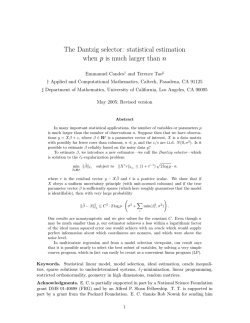
In Figure 5.5 we show two groups of data separated by a thick line (indicating the separating hyperplane H). Parallel to the separating line two others (thin) lines are depicted;
they constitute (delimit) the margin. For the data set exhibited in the figure, each margin
is supported by one support point lying exactly in the margin line; generally, for other
data sets, there could be more support points.
Figure 5.5: Support Vector Machine. The problem of finding the
separating hyperplane with the
largest margin. The data points
belong to 2 classes and are separable. File sv1.jpg
Our goal now is to find the hyperplane (i.e. weight vector a) that maximizes the margin
m (it is believed that the larger the margin, the better generalization of the classifier).
From (5.20) we see that m depends from a : taking smaller a makes the margin
larger. Therefore we assume the additional constraint {constr1}:
m В· a = 1.
(5.21)
Thus, minimizing a we maximize the margin m.
Substituting m := 1/ a , the inequalities (5.20) are converted to {constr2}:
zk g(yk ) ≥ 1, k = 1, . . . , n.
(5.22)
The hyperplane, for which the above inequalities (5.22) hold, is called canonical hyperplane.
Now let us formulate mathematically our optimization problem:
(Problem P1 by Verri [7]). Minimize the weight vector a subject to the constraints (5.22):
Problem P1
Minimize 12 a 2
subject to: zk g(yk ) ≥ 1, k = 1, . . . , n
The solution to our optimization problem is given by the saddle point of the primal
Lagrangian (primal problem) {primal}:
1
L(a, b, О±) = a
2
2
n
в€’
О±k [zk (aT yk + b) в€’ 1 ],
(5.23)
k=1
with αk ≥ 0 denoting the Lagrange multipliers.
The variables to optimize are: the weight vector a and the bias b (primal variables)
and the Lagrange constraints αk , αk ≥ 0, k = 1, . . . , n. We seek to minimize L(..) with
respect to the weight vector a and the bias b; and to maximize it with respect to the 2nd
term on the right (expressing the goal of classifying the points correctly). It may be stated
5 LINEAR DISCRIMINANT FUNCTIONS
37
that the solutions (aв€— , bв€— , aв€— ) lie at a saddle point of the Lagrangian; at the saddle point
a attains its minimum and О± attains its maximum.
Classical Lagrangian duality enables the primal problem (5.23) to be transformed to
its dual problem, which is easier to solve. The dual problem is formulated as
max W (О±) = max { min L(a, b, О±)}
О±
О±
a,b
This means that we find firstly minimum of L(a, b, α) with respect to (a,b) and next –
with the found solution a∗ – we maximize L(a∗ , α) withe respect to α.
We use here so called Kuhn–Tucker theorem, which is an extension of Lagrange’s multiplier method and allows to optimize problems in which the constraints are inequalities.
According to the Kuhn–Tucker theorem, at the solution a∗ , b, the derivatives of L with
respect to the primal variables must vanish, i.e.
∂L(a, b, α)
= 0,
∂a
∂L(a, b, α)
= 0.
∂b
This condition leads to the solution {astar}:
aв€— =
n
О±k zk yk .
(5.24)
k=1
and another constraint nk=1 О±k zk =0. We do not obtain at this stage any solution for b.
Looking at the equation (5.24) one may see that the solution vector aв€— is a linear
combination of the traning vectors, namely those vectors whose О±k are not equal to zero.
Substituting the solution aв€— into (5.23) we obtain the dual problem (Problem P2 in
Verri [7])
Problem P2
Maximize в€’ 12 О±T DО± + nk=1 О±k
n
subject to:
k=1 zk О±k = 0, k = 1, . . . , n
αk ≥ 0,
where
D = {Dij } = {zi zj (yi В· yj )}, (i, j = 1, . . . , n).
The corresponding Lagrangian – to be minimized, thus taken with the ’–’ sign – is {Lp2}
L(О±) = +
1
2
О±k О±j zk zj yjT yk в€’
k,j
n
О±k =
k=1
1 T
О± DО± в€’ 1Tn О±.
2
(5.25)
The Kuhn-Tucker’s theorem implies that the αi ’s must satisfy the so–called Karush–
Kuhn–Tucker (KKT) complementarity conditions, which are formed from the product of the Lagrange multipliers and the corresponding inequality constraints entering the
Lagrangian of the primal problem, taken with an equality sign5 . For our problem this
results in the equality {KT3 }:
О±kв€— [zk g(yk ) в€’ 1] = 0, (k = 1, . . . , n).
5
(5.26)
The Kuhn-Tucker theorem states that the Lagrange parameters can be non-zero only, if the corresponding inequality constraints – entering the primal Lagrangian – taken at the solution, are equality
constraints.
5 LINEAR DISCRIMINANT FUNCTIONS
38
The above condition implies, that either the Lagrange multipliers О±kв€— or the the expression
inside the square brackets [ ... ] have to be zero.
The bracket [ ... ] can be zero only for points lying on the margins, i.e. for the support
points. Then the О±kв€— may be strictly positive.
For other points, not being support vectors and lying beyond the margins, to satisfy
the KKT condition, the multipliers О±k must be equal to 0.
Thus most of the constraints О±k will be equal to zero. Let nSV denotes the number of
support vectors, and SV the set of their indices.
The multipliers О±k s are usually obtained from the Lagrangian (5.25) using the method
of quadratic programming 6 . Let О±в€— denote the solution of problem P2. Then the solution
aв€— given by eq. (5.24) can be rewritten as {astar1}:
aв€— =
О±kв€— zk yk .
(5.27)
kв€€SV
We need still determine the bias b. Is is established from the KKT condition eq. (5.26)
stating that at the solution the following equalities hold:
О±jв€— [zj (aв€— В· yj ) + b) в€’ 1] = 0, (j = 1, . . . , n).
Points, for which the expression in square brackets [...] is equal 0, are support vectors lying
on the margin. Thus we have
zj aв€— В· yj + bв€— zj = 1, в€Ђj в€€ SV,
wherefrom
bв€— = zj в€’ aв€— В· yj .
Taking the average, we obtain (nSV denotes the number of support vectors)
bв€— =
1
nSV
zj в€’
jв€€SV
1 в€—
a В·
yj .
nSV
jв€€SV
Substituting for aв€— the formula (5.27) we obtain
bв€— =
1
nSV
zj в€’
jв€€SV
1
(
О±в€— zk yk ) В·
yj .
nSV kв€€SV k
jв€€SV
Finally {bstar1 }:
bв€— =
1
nSV
zj в€’
jв€€SV
1
О±в€— zk (yk В· yj )].
[
nSV kв€€SV jв€€SV k
(5.28)
Thus, the separating hyperplane is determined only by few data points, the support
vectors. Other data points do not matter, provided that they are located at the proper
side of the hyperplane.
We do not need individual transformed data vectors yk , yj , only their dot product
(yk В· yj ).
6
Matlab offers for that purpose the function quadprog from the Matlab Optimization Toolbox. The
classification toolbox ’Patt’ offers for this purpose two other methods: ’perceptron’ and ’Lagrangian SVM’,
implemented directly inside the procedure ’SVM’
5 LINEAR DISCRIMINANT FUNCTIONS
39
The complexity of the resulting classifier is characterized by the number of support
vectors rather than the dimensionality of the transformed space.
As a result, it may be inferred that SVMs tend to be less prone to problems of overfitting than some other methods.
The support vectors define the optimal separating hyperplane and are the most difficult
pattern to to classify. At the same time they are the most informative for the classification
task.
It may be shown that the upper bound on the expected error rate of the classifier
depends linearly upon the expected number of support vectors.
XOR example.
5.10
Support Vector Machines II. Non-Separable Samples
In the previous subsection, dealing with separable samples, the classifier g(y) has satisfied the following margin inequalities7 :
g(yk ) ≥ +1,
for yk ∈ ω1 (= class C1 ), and g(yk ) ≤ −1,
for yk в€€ П‰2 (= class C2 ),
that – after introducing the target variables zk 8 – were combined together as eq. (5.22)
zk g(yk ) ≥ 1,
The above inequalities were derived on the assumption of separable samples. Now we will
consider the situation, when the training data for class П‰1 and П‰2 are not separable, which
means that they do not satisfy the above inequalities (5.22) stating that zk g(yk ) ≥ 1. Such
a situation is depicted in Figure 5.6. From the configuration of points presented in that
figure, obviously two data points have surpassed their margins and have deviated in the
direction of the opposite class. We have to relax for them the margin inequalities (5.22).
Figure 5.6: The case of nonseparable samples. Values provided by the separating hyperplane g(y) = 0. The data vectors
are allowed to deviate from their
margins (i.e. values g(y) = +1
or g(y) = в€’1) by a slack variable
Оѕ > 0. File sv2.jpg
7
8
in other words, the classifier g(.) is calibrated in such a way that the margin is equal to 1, see eq. 5.22
where zk = +1 for yk в€€ П‰1 (= class C1 ), and zk = в€’1 for yk в€€ П‰2 (= class C2 )
5 LINEAR DISCRIMINANT FUNCTIONS
40
Dealing the case of nonseparable samples, Cortes and Vapnik [9] introduced the following inequalities {ksi}:
zk g(yk ) ≥ 1 − ξk , with ξk ≥ 0, k = 1, . . . , n.
(5.29)
The new introduced variables are called slack variables.
The slack variables allow to take into account all samples that have a geometrical
margin less than 1/ a , and a functional margin (with respect to the function g(.)) less
then 1. For such samples the slack variables Оѕk > 0 denote the difference between the value
g(yk ) and the appropriate margin.
Additionally, we introduce another constraint stating that the sum of the slack variables
is not to big. We express the new constraint in the form
C
Оѕk .
k
The constant C plays here the role of a regularization parameter. The sum k Оѕk expresses
our tolerance in the values of the classifier g for misplaced data vectors (i.e. those that are
on the wrong side of the separating hyperplane).
Now our optimization problem is (problem P3 in Verri [7])
Problem P3
Minimize 12 a 2 + C k Оѕk
subject to: zk g(yk ) ≥ 1 − ξk ,
ξk ≥ 0
Again, to solve the problem, we use the Kuhn–Tucker theorem. The primal form of the
Lagrangian now becomes {Lp3 }:
L(a, b, Оѕ, О±, ОІ) =
1
a
2
2
n
+C
n
Оѕk в€’
k=1
О±k [zk (aT yk + b) в€’ 1 + Оѕk ] в€’
k=1
n
ОІk Оѕk . (5.30)
k=1
which may be rewritten as {Lp3a }:
L(a, b, Оѕ, О±, ОІ) =
n
n
n
n
1
a 2 +C
Оѕk в€’
О±k [zk (aT yk +b) в€’ 1 ] в€’
О±k Оѕk в€’
ОІk Оѕk . (5.31)
2
k=1
k=1
k=1
k=1
The βk ’s are Lagrange multipliers to ensure positivity of the ξ’s. As before, in the
case of separable samples, classical Lagrangian duality enables the primal problem to be
transformed to the dual problem. The dual problem is given by {duall }:
max W (О±, ОІ) = max { min L(a, b, Оѕ, О±, ОІ)}.
О±,ОІ
О±,ОІ a,b, Оѕ
(5.32)
This means that firstly we minimize L with respect to a, b, Оѕ, which results in obtaining
as solution aв€— and eventually Оѕ в€— , and next we maximize W (О±, ОІ) = L(aв€— , b, Оѕ в€— , О±, ОІ) with
respect to О±, ОІ.
Taking the derivatives of L with respect to a, b and Оѕ we obtain
n
∂L
= aв€’
О±k zk yk = 0.
∂a
k=1
n
∂L
=
О±k zk = 0.
∂b
k=1
∂L
= C1n в€’ О± в€’ ОІ = 0.
∂ξ
5 LINEAR DISCRIMINANT FUNCTIONS
41
Equating the derivatives ∂L/∂a to zero we obtain the solution for a∗ , which is the same
as in the separable case (see eq. 5.24)
Equating the derivative ∂L/∂b to zero we obtain the constraint nk=1 αk zk =0, which
again is the same as in the separable case.
Hence
aв€— =
from ∂L/∂a :
О±k zk yk ,
k
n
from ∂L/∂b :
О±k zk = 0
k=1
ОІkв€— = C в€’ О±k , k = 1, . . . , n.
from ∂L/∂ξ :
Taking into account the equality C = α + β and the inequalities α ≥ 0, β ≥ 0 we obtain
that the αk ’s satisfy the so called box constraints {boxconstr }:
∀k 0 ≤ α k ≤ C .
(5.33)
Substituting the βk ’s into the modified Lagrangian (5.31) we state that expressions containing C and ξ do vanish and we are left with the simplified Lagrangian {Lp3simple}:
L(a, b, О±) =
1
a
2
2
n
в€’
О±k [zk (aT yk + b) в€’ 1 ].
(5.34)
k=1
Substituting the solution aв€— into the simplified Lagrangian (eq. (5.34) above) we obtain
the dual problem (Problem P4 in Verri [7])
Problem P4
Maximize в€’ 12 О±T DО± + nk=1 О±k
n
subject to:
k=1 zk О±k = 0, k = 1, . . . , n
0 ≤ αk ≤ C
where
D = {Dij } = {zi zj (yi В· yj )} (i, j = 1, . . . , n)
The dual problem P4 above has the same form as the problem P2 for the separable
case, with the only change that now we have an upper bound on the αk ’s (they satisfy the
box constraints 0 ≤ αk ≤ C).
The corresponding Lagrangian – to be minimized (we have changed the sign) – can be
rewritten as {Lp4 }:
L(О±) =
1
2
О±k О±j zk zj yjT yk в€’
k,j
n
О±k ,
(5.35)
k=1
Again, the Lagrangian (eq. 5.35 above) has the sam form as the corresponding Lagrangian (eq. 5.25) in the separable case, with the only change that now we have an upper
bound on the О±k s. The solution О±в€— can be obtained, e.g., using the method of quadratic
programming (see the comments about solving equation 5.25).
5 LINEAR DISCRIMINANT FUNCTIONS
42
The Karush–Kuhn–Tucker (KKT) conditions are
I :
II :
О±kв€— (zk g(yk ) в€’ 1 + Оѕk ) = 0,
ОІkв€— Оѕk = (C в€’ О±kв€— )Оѕk = 0.
I. Analyzing the first KKT condition, we state that О±i > 0 only when [..]=0.
Patterns, for which О±k > 0 are termed the support vectors. Only these patterns enter
into the evaluation formula for the solution aв€— .
II. Analyzing the second KKT condition, we state that Оѕi > 0 only when C = О±i .
Alternatively (i.e. when О± < C), the slack variables have to be equal to 0.
Considering various values of Оѕi combined with О±i > 0 we have the cases:
• If ξi = 0, the corresponding point is on the margin, because then [zi g(yi ) = 1]
• If 0 < ξi < 1, then we have [0 < zi g(yi ) < 1], the corresponding point yi , although
having a slack, is classified correctly
• If ξ = 1, the point yi is on the separating hyperplane, because then [zi g(yi ) = 1 − 1 = 0].
• If ξ > 1, then [zi g(yi ) < 0], the point yi is on the wrong side of the separating hyperplane
and is evidently wrongly classified.
Define by SV the set of data vectors, for which 0 < αi ≤ C. These vectors are termed
support vectors.
The SV set designates the solution aв€— .
Define by SV the set of data vectors, for which 0 < О±i < C. These data vectors have
slack variables equal to zero and are located on the margin (because they satisfy zi g(yi ) = 1
by the I KKT condition).
The SV set designates the solution bв€— .
The support vectors satisfying 0 < О±k < C must have Оѕk = 0, which means that they
lie on the canonical hyperplane at a distance 1/ a from the separating hyperplane.
Non–zero slack variables can only occur when αk = C. In this case the points yk are
misclassified if Оѕk > 1. If Оѕk < 1, they are classified correctly, but lie closer to separating
hyperplane than the distance 1/ a .
If Оѕk = 0, the point yk is located on the decision boundary and might belong both to
class 1 and class 2.
The only free parameter is C. It may be chosen by varying C through a range of values
and monitoring the performance of the classifier on a separate validation set, or — using
cross validation.
The solution (aв€— ) is the same as in the separable case, see equations 5.27:
aв€— =
О±kв€— zk yk .
kв€€SV
The solution (bв€— ) is derived analogously as in the separate samples case (see equations
5.28), however using data vectors only from the set SV. We obtain then
bв€— =
1
nSV
zj в€’
jв€€SV
1
О±в€— zk (yk В· yj )].
[
nSV kв€€SV jв€€SV k
Again one may see that the evaluation of the classifier g(y) requires only the scalar
products (dot products) yiT y = (yi В· y) and never the underlying values yi and y.
5 LINEAR DISCRIMINANT FUNCTIONS
5.11
43
The kernel trick and MatLab software for SVM
Properties of kernels
The classifier g(y) requires only the evaluation of scalar products (yj В· y) = yjT y, j в€€ SV
and never the pattern y = П•(x) in its explicit form.
When using special functions П•(.) termed kernels, the scalar product can be evaluated
in a simple way as
k(xi , xj ) = П•(xi ) В· П•(xj ).
(5.36)
E.g., using the polynomial kernel k(x, y) = (x В· y)d it can be shown that it corresponds to
mapping x, y into a space spanned by all products of exactly d dimensions.
The formula (5.36) is valid for all kernels satisfying the Mercer’s theorem.
The kernels should satisfy the so called Mercer’s condition (see, e.g., Gunn[5] or ShaweTaylor and Christianini 9 ).
Example of the Polynomial kernel transformation – from Verri [7].
We have 2 points: x = (x1 , x2 ) and y = (y1 , y2 ). From these we construct polynomial
of degree 2:в€љ
в€љ
в€љ
z(x) = (1, в€љ2x1 , в€љ 2x2 , x21 , x22 ,в€љ 2x1 x2 ) and
z(y) = (1, 2y1 , 2y2 , y12 , y22 , 2y1 y2 ).
The corresponding kernel equals
K(x, y) = z(x) В· z(y) = (1 + x В· y)2 .
Software for SVM
The classification toolbox ’Patt’ by David G. Stork and Elad Yom-Tov
The ’Patt’ toolbox [3] uses the kernels:
•
•
•
•
Gaussian (RBF) RBF, one parameter: width of the Gaussian kernel
Polynomial Poly, 1 parameter: polynomial degree
Linear Linear, no parameter needed
Sigmoid Sigmoid, two parameters: [slope constant]
To solve the optimization problems P2 or P4, the function SVM offers the following solvers:
Quadprog, taken from the MatLab Optimization Toolbox vs. 6;
Perceptron, implemented directly inside the function ’SVM’; the weights are updated using
the worse classified pattern;
Lagrangian, algorithm from Mangasarian & Musicant, Lagrangian Support Vector Machines.
The function SVM may be used from the GUI, or directly by writing some macro
instructions in MatLab.
The GUI can be used only for 2-dimensional data; then we obtain a graphical visualization of the decision boundary, of the margins and support vectors.
When using data with more then d=2 variables, we obtain only numerical results, which
eventually we might visualize using own macros.
An example of calculations using own macro:
9
J. Shawe-Taylor and N. Christianini, Kernel Methods for Pattern Analysis, Cambridge University
Press, 2004
5 LINEAR DISCRIMINANT FUNCTIONS
44
% calculations using SVM from ’Patt’
% needs data of size (nxd), y of size(nx1)
% y has elements ’0’ and ’1’
C=300: % slack variable, can be ’inf’
par=’[’’Poly’’,2,’’Quadprog’’,C]’;
[test_targets,a_star]=SVM(data’,z’,data’,par);
length(find(z’~=test_targets’))
S=find(z’~=test_targets’);
disp([num2str(length(S)), ’ misclassified]’)
The svm toolbox developed by Steve Gunn
This toolbox [5] offers for use the following kernels:
%
%
%
%
%
%
%
%
%
Values for ker: ’linear’
’poly’
’rbf’
’sigmoid’
’spline’
’bspline’
’fourier’
’erfb’
’anova’
-
p1 is degree of polynomial
p1 is width of rbfs (sigma)
p1 is scale, p2 is offset
p1
p1
p1
p1
is
is
is
is
degree of bspline
degree
width of rbfs (sigma)
max order of terms
The parameters of the kernel functions are denoted by p1 and p2 and are global variables.
The calculations may be performed using the graphical GUI called ’uiclass’, which
– when called the first time – sets the global variables p1 and p2. The GUI may use the
user’s data, e.g.:
% data should be in MAT format,
% declaration of global variables is not necessary
% X=data; Y=z; save and2.mat X Y -mat;
uiclass %activates gui, which asks for data in the ’.mat’ format
Alternatively, The calculations may be performed using a macro written directly
by the user. An example:
ker=’poly’; C=300; % ’linear’, ’rbf’, ’sigmoid’; inf
[nsv, alpha, b0] = svc(data,z,ker,C);
[predictedY,err] = svcerror1(data,z,data,z,ker,alpha,b0);
mis=find(z~=predictedY);
disp([num2str(length(mis)), ’ misclassified’])
[h] = svcplot(data,z,ker,alpha,b0);% plots only 2-dimensional data
The ’data’ should have the size (nxd), the ’z’ vectors of size (nx1) represents the target
vectors, and is composed of elements ’1’ and ’-1’ denoting the 1st and 2nd class appropriately. The visualization is only possible for two-dimensional data.
6 MIXTURE MODELS
6
45
Mixture models
Defining the mixture model
Let t = (t1 , . . . , td )T denote an observational vector, t в€€ Rd . Generally, t has a probability
distribution p(t) characterized by a set of parameters Оё:
t в€ј p(t) = p(t; Оё) .
E.g. the probability distribution might be the normal distribution Nd (Вµ, Пѓ 2 ) with parameters Оё = ((Вµ), Пѓ 2 ).
In practice we may have difficulties to model the observed data using a single distribution p(t, Оё. However, often we may do it assuming that the observed data represent
de facto M different groups of data; each group (j) is modelled by the same probability
distribution p(t), using different parameter set (Оё j ). This may be written as the mixture
model {mix1}
M
ПЂj = 1
πj p(t|θ j ) , πj ≥ 0,
p(t) =
(6.1)
j
j=1
where
πj – denotes the jth mixing proportions, j = 1, . . . , M ,
p(t|θ j ) – denotes the probability distribution function governing the jth group.
How many parameters characterize the mixture?
We have to know
•
•
•
•
M , the number of components of the mixture
p(t|j), the functional form of the distribution of t in the jth group,
Оё j , the parameters characterizing the conditional distribution function p(t|j; Оё j ),
ПЂ1 , . . . , ПЂM , the mixing coefficients.
Often we assume a given value of M . We assume also the general shape of the distribution function p(t|j; .). The remaining task is then to estimate the values of the parameters
Оё 1 , . . . , Оё M and ПЂ1 , . . . , ПЂM .
Estimation of the parameters
For an independent sample of N vectors, (t1 , . . . , tN ) drawn from the distribution p(t, Оё)
we have {tsample}
tn в€ј p(tn ; Оё), n = 1, . . . , N.
(6.2)
We seek for such values of the parameters which maximize the likelihood {L}
N
N
L=
M
p(tn ) =
n=1
p(tn |j; Оё j ) ПЂj .
(6.3)
n=1 j=1
Usually the solution (i.e. the estimates of the parameters) are obtained by seeking for the
minimum of the error function E, which is defined as the negative logaritm в€’lnL {logL}
N
E = в€’lnL = в€’
N
ln p(tn ) = в€’
n=1
M
ln
n=1
p(tn |j; Оё j )ПЂj .
j=1
(6.4)
6 MIXTURE MODELS
46
The error function E, to be minimized, is a function of the parameters
E = E(t1 , . . . , tN ; Оё 1 , . . . , Оё M , ПЂ1 , . . . , ПЂM ),
with the linear constraint
M
j=1
ПЂj = 1.
We know from the general optimization theory that at the solution the gradients with
respect to the parameters should be equal to zero. This yields the following set of equations
∂E
= 0, (j = 1, . . . , M ),
∂θ j
∂E
= 0, (j = 1, . . . , M ).
∂πj
The solution is obtained in an iterative way and is usually complicated. Usually we solve
the equations using the EM algorithm.
For isotropic Gaussian distributions we may obtain a relatively simple explicit solutions
which are adjustable sequentially.
The EM algorithm
We suppose that we have a set of ’incomplete’ data vectors {x} and we wish to maximize
L(ОЁ) = p(x|ОЁ) where ОЁ = [ПЂ1 , . . . , ПЂM ; Оё 1 , . . . , Оё M ].
Let
where zi = (z1i , . . . , zM i )T is defined the following way
yiT = (xTi , zTi ),
zji =
1,
0,
if xi belongs to the jth component,
otherwise.
The EM algorithm is based on the likelihood function and proceeds in two steps:
The E-step – Expectation. We seek for the expectation of the missing values zj .
The M-step – Maximization. We maximize the likelihood L substituting for the missing
values the estimates found in the E–step.
Software
Netlab [10] is a very reliable software for calculating the mixtures.
To get familiar, one may run the demo examples.
demnlab
Choose the section ’Density Modelling and Clustering’
run the examples ’full’, ’diagonal’, ’spherical’, ’EM’
’Neuroscale’ and ’GTM’ are methods for visualization of multivariate data in a plane using
a mixture of RBF functions.
The demos for these methods may be accessed independently from the gui running ’demns1’
and ’demgtm2’ from the command window.
The demo ’demmlp2’ demonstrates the use of mixtures when building an Bayesian
classifier. The performance of the constructed Bayesian classifier is compared with that
obtained when using a multilayer perceptron (MLP).
7 COMPARING AND COMBINING CLASSIFIERS
7
47
Comparing and combining classifiers
1.
2.
3.
4.
5.
6.
7.
8.
7.1
Mc Nemar’s test
ROC curve
Averaging results provided by Committees of networks
Re-sampling, Bootstrap, Bagging
Stacked generalization
Mixture of experts
Boosting
Model comparison by Maximum Likelihood
Statistical tests of equal error rate
After Webb [2], p. 267.
Let A and B be two classifiers trained on a train set Dtrain and tested on a test set Dtest .
Consider now the performance of the two classifiers on the test set Dtest .
Let: n00 – nb of misclassified vectors by both A and B,
n01 – nb of misclassified vectors by A but not A,
n10 – nb of misclassified vectors by B but not by A,
n11 – nb of misclassified vectors by neither A nor B.
To test whether the differences between the counts {nij , i, j = 0, 1} are statistically
significant, we apply the Mc Nemar’s test. Calculate the statistics
z=
|n01 в€’ n10 | в€’ 1
в€љ
.
n01 в€’ n10
Under the null hypothesis that both classifiers have the same error rate, the statistics z
has П‡2 distribution with 1 degree of freedom:
z|H0 в€ј П‡21 .
7.2
The ROC curve
The ROC curve was described in Section 2. We are specially concerned with properly
recognizing one group of data, e.g. computer attacks.
Say, we have L classifiers serving this purpose. We may depict the behavior of these
classifiers (the ability of detecting ’false positives’ and ’true positives’) in one graph displaying the respective ROC curves.
7 COMPARING AND COMBINING CLASSIFIERS
7.3
48
Averaging results from Committees of networks
Text based on Bishop, p. 364–369
We train several (L) candidate networks and next combine their results with the hope
that this will lead to significant improvements in the predictors on new data, while involving
little additional computational effort. We hope also that the performance of such combining
will be better than the performance of the best single network.
Let yi (x) be the prediction done by the i-th network (i = 1, . . . , L).
We have:
yi (x) = h(x) + i (x),
where h(x) is the due value of the prediction and i (x is the error (deviation from h(x))
observed for given x.
Let Ei = E[{yi (x) в€’ h(x)}2 ] = E[ 2i ] be the expected error of the ith prediction. Then the
average of the expected errors of the L predictors is
EAV = L1 Li=1 Ei = L1 Li=1 E[ i ]2 . Thus
1 L
=
E[ i ]2 .
L i=1
EAV
This is the average error of the expected predictions by each of the L networks.
Now let us consider the prediction yCOM obtained by averaging the L predictions. We
have
1
ECOM = E[(
yi (x) в€’ h(x))2 ] = E[ 2i ].
L
Assuming E[ i ] = 0, E[ i j ] = 0, i = j, we obtain
ECOM
1
= 2
L
L
E[( i )2 ] =
i=1
1
EAV .
L
The formula above was derived under the assumption that the errors are independent and
uncorrelated. This is not always true. However, we may also derive the formula above
using the Cauchy inequality
L
(
( i )2 ) ≤ L
i=1
L
2
i.
i=1
Using this inequality we obtain
ECOM ≤ EAV .
We might also ask, whether taking generally a weighted linear combination of the predictions yi we might further reduced error. The problem, and how to solve it, is described
in Bishop [ ]. In any case we have
EGEN ≤ EAV ,
where EGEN denotes the expected error of the linear combination
L
yGEN (x) =
L
О±i yi (x), with
i=1
О±i = 1.
i=1
7 COMPARING AND COMBINING CLASSIFIERS
7.4
49
Re-sampling: bootstrap and bagging
Bootstrap
We perform the calculations using resampling with replacement. The process of resampling
Л† в€—(.) ,
is repeated B times. Let Оё be the statistic of interest. Then the bootstrap estimate Оё
of the statistic Оё, is simply the mean of the B estimates on the individual bootstrap data
sets:
в€—(.)
1 B Л†в€—(b)
ОёЛ† =
Оё .
B b=1
Bootstrap variance estimate
V arboot =
1
B
B
в€—(b)
[ОёЛ†
в€—(.)
в€’ ОёЛ† ]2 .
b=1
If the statistic Оё is the mean, then in the limit of B в†’ в€ћ, the bootstrap estimate of the
variance is the traditional variance of the mean.
Generally speaking, the larger the number B of bootstrap samples, the more satisfactory
is the estimate of a statistic and its variance.
Bagging
Bagging (from: ’bootstrap aggregation’, see Duda p. 476) uses multiple versions of a
training set, each created by drawing n < n samples from D with replacement.
Each of these bootstrap data sets is used to train a different component classifiers and
the final decision (classification decision) is based on the vote of each component classifiers.
Traditionally, the component classifiers are of the same general form; merely the final
parameter values differ among them due to their different sets of training parameters.
A learning algorithm carried out on a data set may be ’unstable’ if ’small’ changes in the
data lead to significantly different classifiers and relatively ’large’ changes in accuracy. In
general, bagging improves recognition for unstable classifiers because it effectively averages
over such discontinuities. There are no convincing theoretical derivations or simulation
studies showing that bagging will help all unstable classifiers, however (quoted after Duda,
p.476).
The global decision rule in bagging – a simple vote among the component classifiers
– is the most elementary method of pooling or integrating the outputs of the component
classifiers.
7.5
Stacked generalization
After Webb [2], p. 290.
Let: D – the (training) data set, L – nb. of classifiers, V – nb of partitions of the data,
{xi }, {ti }, i = 1, . . . , n – the patterns and corresponding targets contained in D.
Divide the data set D into V partitions.
Execute for v = 1, . . . , V
a) train the classifier no. j (j = 1, . . . , L) on all training data except partition v, thus
obtaining the classifier (classification rule) gj(в€’v) ;
b) test each classifier, gj(в€’v) , on all patterns in partition v.
7 COMPARING AND COMBINING CLASSIFIERS
50
This produces a data set of L predictions, gj (xi ), on each pattern (xi ) contained in the
training data set.
Then we have the following data:
Training
x1 ,
x2 ,
. .
xn ,
set
t1
t2
.
tn
New set
g1 (x1 ),
g1 (x2 ),
. .
g1 (xn ),
(predictions)
. . . , gL (x1 )
. . . , gL (x2 )
.
. . . , gL (xn )
We may now take the set gj (xi ), (j = 1, . . . , L; i = 1, . . . , n) as predictors and ti as
targets and build a new prediction rule. In case, when the predictors are categorial (no.s
of assigned classes), this may be done by correspondence analysis. Merz (1999) has done
this with an approach based on a multivariate analysis method (correspondence analysis).
7.6
Mixture of experts
The method was proposed by Jacobs et al., 1991. see Webb [2], p. 291.
We consider the problem of mapping in which the form of the mapping is different for
different regions of the input space. We assign different expert networks to tackle each of
the different regions and also an extra gating network which sees also the input vector, to
decide which of the experts should be used to determine the output. The experts and the
gating network are determined as part of the learning process.
The system is depicted in Figure 7.1.
The goal of the training procedure is to have the gating network learn an appropriate
decomposition of the input space into different regions, with one of the expert networks
responsible for generating the outputs for input vectors falling within each region.
The gating network is trained simultaneously with the constituent classifiers. The
gating network provides a ’soft’ partitioning of the input space, with experts providing
local predictions.
In the basic approach, the output of the ith expert, oi (x), is a generalized linear function
of the input, x
oi (x) = g(x; Оё i )
where Оё i is the vector of parameters associated with the ith expert and g(.) is a fixed
nonlinear function.
The gating network is also a generalized linear function, w, of the input x. The gating
network sees the input and makes a soft partitioning of the input space, into L parts, by
assigning a proper weight to the given x. The weight for the ith component network is
assigned by the function softmax as
wi = w(x, О±i ) =
exp(О±Ti x)
, i = 1, . . . , L.
L
T
k=1 exp(О±k x)
These outputs of the gating network are used to weight the outputs of the experts to give
the overall output, o(x), of the mixture of experts
L
o(x) =
wk ok (x).
k=1
7 COMPARING AND COMBINING CLASSIFIERS
51
Figure 7.1: Mixture-of-experts. The architecture consists of k component classifiers or
’experts’, each of which has trainable parameters θ i , i = 1, . . . , k. For each input x each
component classifier i gives estimates of the category membership gir = P (П‰r |x, Оё i ). The
outputs are weighted by the gating subsystem governed by parameter vector Оё 0 and are
pooled for ultimate classification. Graph and description from Duda et al., p. 496. File
duda9 19.jpg
The toolbox ’Patt’ offers two functions for mixtures of experts:
Components with DF – the outputs ok (x) of the components are calculated using the logistic discriminant function;
Components without DF – the outputs ok (x) of the components are calculated using declared classifiers gk (x; θ k ).
7.7
Boosting, AdaBoost
Proposed by Freund and Schapire (1996), boosting assigns a weight to each pattern
in the training set, reflecting its importance, and constructs a classifier using the training
set and the set of weights. As compared with bagging, it generates the training sets
sequentially, based on the results of the previous iteration. In contrast, bagging generates
the training set randomly and can generate the classifiers in parallel.
General description in [3]: AdaBoosts builds a nonlinear classifier by constructing an
ensemble of ’week’ classifiers (i.e. ones that need perform only slightly better than chance)
so that the joint decision has better accuracy on the training set. It is possible to iteratively
add classifiers so as to attain any given accuracy on the training set. In AdaBoost each
sample of the training set is selected for training the weak with a probability proportional
to how well it is classified. An incorrectly classified sample will be chosen more frequently
for the training, and will thus be more likely to be correctly classified by the new classifier.
Additional inputs: The number of boosting iterations, the name of week learner and
its parameters.
The AdaBoost algorithm implemented in the classification toolbox ’Patt’ works according the scheme described in [3], p. 112. The same algorithm, slightly modified, is presented
in Table 7.1.
7 COMPARING AND COMBINING CLASSIFIERS
52
Table 1: The AdaBoost algorithm after Duda et al. [1], p.478.
AdaBoost()
1 input D = {xi , yi }, i = 1, . . . , n, kmax
2 initialize W1 (i) = 1/n, i = 1, . . . , n,
3 k в†ђ 0;
4 repeat
5
k в†ђk+1
6
train weak learner Ck using Dk sampled from D according to Wk (i)
7
Ek в†ђ training error of Ck measured on D using Wk (i)
8
break if Ek = 0 {or Ek ≥ 0.5}
9
О±k в†ђ 12 ln[(1 в€’ Ek )/Ek ]
e в€’ О±k if gk (xi ) = yi
10
Wk+1 (i) в†ђ WZkk(i) Г—
e О±k
if gk (xi ) = yi
11
Zk is a normalizing constant
12
13
until k в†ђ kmax
14 return Ck and О±k for k = 1, . . . , kmax (ensemble of classifiers with weights)
15 The value of the final AdaBoost classifier for a new x is then estimated as
max
Л†
16
C(x)
= kk=1
ln[(1 в€’ Ek )/Ek )] Ck (x]
Initially, all samples are assigned equal weights wi = 1/n. At each stage (k) a classifier
(Ck ) is constructed using the actual weights Wk (line 5).
Then the error Ek , taken as the sum of weights of misclassified vectors from the training
set, is calculated (line 6), and an error factor О±k (line 7).
Next the weights of misclassified patterns are increased – by multiplying them by a
factor exp(αk ) – and the weights of correctly classified patterns are decreased – by multiplying them by a factor exp(αk ). This stage is described as ’boosting’ the weights. The
boosting should be applied only when Ek < 0.5. The effect is that in the next iteration
(k + 1) the higher weight pattern will influence the learning classifier more, and thus cause
the classifier focus more on the misclassification. Generally those are patterns that are
nearest to the decision boundary.
The performance of the boosting in subsequent iterations is illustrated in Figure 7.2
(extracted from Raetsch et al., Soft margins for AdaBoost, Machine Learning 42(3), 287–
320, March 2001). We may see in that Figure the evolution of the AdaBoost algorithm.
Another illustration of the performance of the AdaBoost algorithm using the ’Patt’
toolbox is shown in Figure 7.3, left. The plot shows the ’four spiral’ data containing 1000
data points and subdivided into 2 classes.
Call of the function AdaBoost in ’Patt’:
[test targetsP, E] = ada boost(train patterns, train targets, test patterns, params);
The function makes break if Ek = 0, however does not make break when Ek ≥ 0.5.
The plot of error E calculated in subsequent iterations is shown in Figure 7.3, right;
we see here oscillations around the value E = 0.5 beginning from about the 10th iteration.
The decision boundary (drawn by the classifier’s GUI) is shown in Figure 7.3, left.
7 COMPARING AND COMBINING CLASSIFIERS
53
Figure 7.2: Illustration of AdaBoost using a 2D toy data set: The color indicates the
label and the diameter is proportional to the weight of the patterns. Weighted patterns in
the first, second, third, 10th and 100th iterations are shown. The dashed lines show the
decision boundaries of the single classifiers (up to the 5th iteration). The solid line shows
the decision line of the combined classifier. In the last two plots the decision line obtained
from Bagging is shown for comparison. Figure taken from Raetsch et.al. 2001. File rae.jpg
Weighted average train error
0.65
0.6
0.55
0.5
0.45
0.4
0.35
0.3
0.25
0.2
0
10
20
30
40
50
60
70
80
90
Iteration No.
Figure 7.3: AdaBoost for the four spiral data. Learner: RBF network with 12 RBF centers.
Left: Decision boundaries after 100 iterations. File rbf100j.jpg. Right: Misclassification
error for the training data set (taken without weights) noticed in subsequent 100 iterations.
File rbfErr100.eps
100
7 COMPARING AND COMBINING CLASSIFIERS
7.8
54
Model comparison by Maximum Likelihood
Figure 7.4: The evidence (i.e. probability of generating different data sets given a model)
is shown for three models of different expressive power or complexity. Model h1 is the most
expressive, because with different values of its parameters the model can fit a wide range of
data sets. Model h3 is the most restrictive of the three. If the actual observed data is D(0) ,
then the maximum likelihood model selection states that we should choose h2 , which has
the highest evidence. Model h2 ’matches’ this particular data set better than do the other
two models, and it should be selected. Graph and description from Duda et al., p.487. File
duda9 12.jpg
8 VISUALIZATION OF HIGH-DIMENSIONAL DATA
8
55
Visualization of high-dimensional data
8.1
8.1.1
Visualization of individual data points using Kohonen’s SOM
Typical Kohonen’s map
The method of Kohonens’ self-organizing mas is a non-linear method of projection of data
from a multi-dimensional space onto (usually) a plane called the ’map’. The data vectors
are represented by their representatives, called codebooks or prototypes. We do not obtain
projections of individual data vectors. The map is a stiff one. The projections reflect only
the topological neighborhood of the prototypes and not their true distances. However,
the u–mat technique permits – by using color painting – to depict in a specific way the
approximate distances between neighboring prototypes.
8.1.2
The new method proposed by Liao et.al. 2003
The proposed method permits to project individual data points.
8.1.3
Example 1, Synthetic
8.1.4
Example 2, monitoring gearbox condition
8.1.5
Example 3, visualization of the LowHi erosion data
8.2
The concepts of volume, distance and angle in multivariate
space
Some weird facts about the concepts of ’volume’, ’distance’ and ’angle’ in multivariate
space may be found in the papers by Verleysen et al. and Herault et al. (see references
below).
8.3
CCA, Curvilinear Component Analysis
Based on the papers by Herault et al. – see references below.
8.3.1
The principle of CCA
8.3.2
Scene classification
An image is analyzed by a bank of spatial filters, according to four orientation and 5
frequency bands, ranging from very low spatial frequencies to medium ones. The global
energies of the 20 filters’ outputs constitute a 20–dimensional feature space. Using CCA,
Herault et.al. obtained the visualization shown in Figure 8.9. The obtained organization
of the data is in surprising accordance with some semantic meaning: Natural/Artificial for
each side of the grey line, and and Open/Closed along this line.
1. J. Herault, A. Guerin–Dugue, P. Villemain, and unsolved questions. ESANN’2002 proceedings, Bruges (Belgium), d-side publi., 173–184.
2. J. Herault, Aude Oliva, Anne Guerin-Dugue, Scene Categorisation by Curvilinear Component Analysis of Low Frequency Spectra. ESANN’1997 proceedings, Bruges (Belgium),
d-side publi., 96–96.
8 VISUALIZATION OF HIGH-DIMENSIONAL DATA
56
3. G. Liao, S. Liu, T. Shi and G. Zhang, Gearbox condition monitoring using self-organizing
feature maps. Proc. Instn. Mech. Engrs Vol. 218 Part C, 119–129. J. Mechanical
Engineering Science, c IMechE 2004,
4. M. Verleysen, D. FranВёcois, G. Simon, W. Wertz, On the effects of dimensionality on data
analysis with neural networks. J. Mirra (Ed.): IWANN 2003, LNCS 2687, 105–112.
5. M. Verleysen, Machine Learning of High-Dimensional Data, PHD Thesis, Universite Catholique
de Louvain, Laboratoire de Microelectronique, Louvain-la-Neuve, 2000.
lowHi 4x4Hits
Liao, data: Erosion Low and High
4
3.5
3
low
high
2.5
2
1.5
1
1
1.5
2
2.5
3
3.5
4
lowHi
lowHi
Figure 8.1: Erosion data LowHigh. Left: Kohonen map. Right: Liao’ visualization. Files
maplow.eps, liaoLH.eps
3D data: Erosion Low and High
Erosion Low High lambda=54.179
2
low
high
low
high
1.5
1
1
Canonical Discr. Variate no. 2
0.5
0
в€’0.5
в€’1
в€’1.5
0.5
0
в€’0.5
в€’2
1.5
1
2
0.5
в€’1
1
0
0
в€’0.5
в€’1
в€’1
в€’1.5
в€’2
в€’1.5
в€’2
в€’1.5
в€’1
в€’0.5
0
Canonical Discr. Variate no. 1
0.5
1
Figure 8.2: Erosion data LowHigh. Left: 3D plot. Right: Canonical discrimination. Files
3DLH.eps, canLH.eps
Full version of Chapter 8 may be found in a separated file entitled ’roadmap8’.

13.4 THE CROSS PRODUCT The Area of a Parallelogram Definition

Document

102M Lab Manual - Department of Physics - The University of Texas

Name_________________________________________

The Dantzig selector - Department of Statistics

Vector Webinar: AUTOSAR Configuration Process - How to handle

Optimisation and Inverse Problems in Imaging

Brochure - X Joint Annual Conference of ISMOCD IAE

Chapter 8. Classification: Basic Concepts

2014 Technical Notes

Using R for Data Analysis and Graphics - The Comprehensive R

WRspice Reference Manual - Whiteley Research Inc.

Manual genie pro max.pdf

cattle futures co

ngspice user manual - SourceForge

Captain underpants book o fun 1.pdf