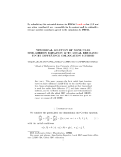
Advances in Applied Mathematics and Mechanics Adv. Appl. Math. Mech., Vol. 7, No. 1, pp. 13-30 DOI: 10.4208/aamm.2013.m359 February 2015 Solution of Two-Dimensional Stokes Flow Problems Using Improved Singular Boundary Method Wenzhen Qu and Wen Chen∗ Department of Engineering Mechanics, College of Mechanics and Materials, Hohai University, Nanjing 210098, China Received 27 September 2013; Accepted (in revised version) 29 June 2014 Available online 23 September 2014 Abstract. In this paper, an improved singular boundary method (SBM), viewed as one kind of modified method of fundamental solution (MFS), is firstly applied for the numerical analysis of two-dimensional (2D) Stokes flow problems. The key issue of the SBM is the determination of the origin intensity factor used to remove the singularity of the fundamental solution and its derivatives. The new contribution of this study is that the origin intensity factors for the velocity, traction and pressure are derived, and based on that, the SBM formulations for 2D Stokes flow problems are presented. Several examples are provided to verify the correctness and robustness of the presented method. The numerical results clearly demonstrate the potentials of the present SBM for solving 2D Stokes flow problems. AMS subject classifications: 76D07, 76M25 Key words: Singular boundary method, origin intensity factor, Stokes flow, fundamental solution. 1 Introduction The incompressible viscous flow in slow motion, known as Stokes flow, is a classical problem in fluid dynamics. It can be regarded as a subset of Navier-Stokes flows, and has been widely applied in the industry. For the numerical analysis of Stokes flow problem, three formulations are well-known: vorticity-stream vector function, vorticity-velocity approach and primitive variable (velocity-pressure) approach. Many numerical methods have been applied to the solution of the Stokes equations, such as finite difference method (FDM) [1], finite element method (FEM) [2] and boundary element method (BEM) [3]. More recently, with the development of the meshless ∗ Corresponding author. Email: [email protected] (W. Chen) http://www.global-sci.org/aamm 13 c 2015 Global Science Press 14 W. Z. Qu and W. Chen / Adv. Appl. Math. Mech., 7 (2015), pp. 13-30 method, some other simpler and fast methods have appeared in the literature, particularly the method of fundamental solution (MFS) which has been used to solving Stokes flow problems [4–6]. Over the last decade, the main advantage of the MFS, namely the simple computational implementation, has been recognized. However, a fictitious boundary for the distribution of source points is required in the MFS, which enormously restricts its application in the practical project. Some efforts have been put in the elimination of this drawback, and numerous techniques are developed. A comprehensive review with respect to these methods can be found in the [7–9]. In this work, we focus on the singular boundary method (SBM), recently proposed by Chen and his collaborators [8, 10, 11]. For the SBM, the source and collocation points are both distributed on the physical boundary, thus there is no need of fictitious boundary required in the MFS. But, the singularity of the fundamental solution is caused when the source point coincides with the collocation point. To isolate the singularity of the fundamental solution, the origin intensity factor is introduced, and thus how to determine the factor is the key issue of the SBM. Prior to this study, the SBM has since been successfully applied to potential [8] and elasticity problems [11], in which we find that the method has a well performance. The object of this paper is to extend the SBM for solving Stokes flow problems. Different from our previous SBM solution of 2D elasticity problems [11], a new regularization technique can accurately remove the singularities of the fundamental solution and its derivatives, and consequently, the origin intensity factors can be determined directly without requiring sample nodes as in [11]. Furthermore, based on the corresponding origin intensity factors, the SBM formulations for the velocity, traction and pressure are established. The rest of this paper is organized as follows. In Section 2, the governing equation of the Stokes problems is introduced, and the origin intensity factors for the velocity, traction and pressure are derived. Section 3 provides four numerical examples to assess the performance of the proposed SBM scheme. Finally, some conclusions are provided in Section 4. 2 The SBM formulation for Stokes problems In this paper, we always assume that Ω is a bounded domain in R2 , Ωe is its open complement; Γ = ∂Ω denotes their common boundary; n(x) and t(x) are the unit outward normal vector and tangential vector of Γ to domain Ω at point x, respectively. Assuming the incompressibility for the fluid medium, the governing equation for the steady-state Stokes flow problems can be expressed as follows: Momentum equation : − p,i + µui,jj = 0, Continuity equation : ui,i = 0, Boundary condition : x ∈ Ω, x ∈ Ω, ui = u¯ i , x ∈ Γu , ti = t¯i , x ∈ Γt , (2.1a) (2.1b) (2.1c) W. Z. Qu and W. Chen / Adv. Appl. Math. Mech., 7 (2015), pp. 13-30 15 where ui is the velocity, p the pressure, µ the coefficient of viscosity of the fluid, u¯ i and t¯i the given values of velocity ui and traction ti on the boundary Γu and Γt (Γ = Γu ∪ Γt ) respectively, and i, j = 1,2. The stress σij (i, j = 1,2) in the fluid can be written as σij = − pδij + µ(ui,j + u j,i ), x ∈ Ω, (2.2) and traction ti (i = 1,2) on Γ can be expressed as ti = σij n j , x ∈ Γ, (2.3) where n j is the component of the outward normal vector n. Employing indicial notation for coordinates of points x and s, i.e., x1 , x2 and s1 , s2 , respectively, the fundamental solutions of the Stokes equation are given as [6] 1 − δij lnr(x,s)+ r,i (x,s)r,j (x,s) , 4πµ 1 r,i (x,s) , Pi (x,s) = 2π r(x,s) Uij (x,s) = i, j = 1,2, (2.4a) i = 1,2, (2.4b) where r(x,s) is the Euclidean distance between the collocation point x and source point s, r,i (x,s) = ∂r(x,s) xi − si = ∂xi r(x,s) expresses the derivative of the distance r with respect to xi , and δij is the Kronecker symbol. Making use of the Eqs. (2.2)-(2.4b), the fundamental solutions of the traction and stress can be respectively expressed as 1 r,i (x,s)r,j (x,s)r,k (x,s)nk (x), πr 1 Dijk (x,s) = − r,i (x,s)r,j (x,s)r,k (x,s), πr Tij (x,s) = − i, j,k = 1,2, (2.5a) i, j,k = 1,2. (2.5b) The SBM uses the fundamental solution as the basis function of its approximation, which is similar to the MFS [7, 12–14]. However, unlike the MFS, the collocation points and source points of the SBM are coincident and placed on the physical boundary, as seen in Figs. 1(a) and (b). For the SBM, we have a fundamental assumption [11, 15] which is the existence of the origin intensity factor upon the singularity of the coincident sourcecollocation nodes for mathematically well-posed problems. With the help of the above assumption, the SBM interpolation formulations for 2D 16 W. Z. Qu and W. Chen / Adv. Appl. Math. Mech., 7 (2015), pp. 13-30 (a) (b) Figure 1: The source (collocation) point distributions: (a) for interior problems, (b) for exterior problems. Stokes flow problems can be expressed as u i ( xm ) = N α j (sn )Uij (xm ,sn )+ α j (sm )uij (xm ), (2.6a) α j (sn ) Tij (xm ,sn )+ α j (sm )tij (xm ), (2.6b) α j (sn ) Pj (xm ,sn )+ α j (sm ) p j (xm ), (2.6c) ∑ n =1,n = m ti ( xm ) = N ∑ n =1,n = m p( xm ) = N ∑ n =1,n = m where α j (sn ) is the unknown coefficient, xm and sn are the mth collocation point and the nth source point, respectively. uij (xm ), tij (xm ), p j (xm ) are defined as the origin intensity factors, namely diagonal and sub-diagonal elements of the SBM interpolation matrix. 2.1 The calculation of uij (xm ) As the collocation point xm approaches to the source point sn , the distance between these two boundary nodes trends to zero, which would cause different orders of singularities in Eqs. (2.6a)-(2.6c). By adopting an average value of the fundamental solution over a portion of the boundary, the calculated formulation of uij (xm ) can be expressed as uij (xm ) = = 1 Lm Γm Uij (xm ,s)dΓ(s) 1 − δij 4πµLm Γm lnr(xm ,s)dΓ(s)+ Γm r,i (xm ,s)r,j (xm ,s)dΓ(s) , (2.7) where Lm indicates the half distance between the source point sm−1 to the source point s m +1 . W. Z. Qu and W. Chen / Adv. Appl. Math. Mech., 7 (2015), pp. 13-30 17 Obviously, the second integral at the right side of Eq. (2.7) has no singularity, and thus it can be accurately calculated by using the standard Gaussian quadrature. But, the following special treatment is required for the first integral which has the weak singularity Γm lnr(xm ,s)dΓ(s) = = 1 −1 1 −1 J (ξ ) lnr(xm ,ξ )dξ [ J (ξ )− J (η )] ln r(xm ,ξ )dξ + J (η ) 1 −1 lnr(xm ,ξ )dξ, (2.8) in which ξ is the intrinsic coordinate that transforms the integral so that it is mapped onto the interval [−1,1], η ∈ [−1,1] represents the position of xm , and J (ξ ) denotes the Jacobian of the transformation. Now, the two integrals at the right side of Eq. (2.8) can be well calculated by using the standard Gaussian quadrature and analytical technique, respectively. 2.2 The calculation of tij (xm ) By using a subtracting and adding-back technique [16], the SBM traction formulation for interior problems can be re-expressed as follows N N ti (xm ) = ∑ α j (sn ) TijI (xm ,sn ) = n =1 α j (sn )− ∑ n =1,n = m + Ln α j (xm ) TijI (xm ,sn ) Lm α j ( xm ) N Ln TijI (xm ,sn )+ Ln TijE (sn ,xm ) , Lm n∑ =1 (2.9) where N ∑ Ln TijE (sn ,xm ) = 0, (2.10) n =1 and Ln is the half distance between source nodes sn−1 and sn+1 , the superscript I and E denote the interior domain problem and the exterior domain problem, respectively. The derivations of Eq. (2.10) are given as in Appendix. Based on the dependency of the outward normal vector on two kernel functions of interior and exterior problems [17], one can obtain the following relationship TijI (sn ,xm ) = κTijE (sn ,xm ), (2.11) where κ is equal to 1 as m = n and is equal to −1 as m = n. Substituting (2.11) into (2.9), we have ti ( xm ) = N ∑ n =1,n = m α j (sn ) TijI (xm ,sn )− α j ( xm ) Lm N ∑ n =1,n = m Ln TijI (sn ,xm )− χIm , (2.12) 18 W. Z. Qu and W. Chen / Adv. Appl. Math. Mech., 7 (2015), pp. 13-30 in which χIm = Lm TijI (xm ,sm )+ Lm TijI (sm ,xm ). (2.13) The terms TijI (xm ,sn ) and TijI (sn ,xm ) in Eq. (2.12) are regular and can be calculated directly because xm and sn are not coincident, i.e., n = m. The remaining term χIm can be approximated as the following integral χIm ≈ Γm TijI (xm ,s)+ TijI (s,xm )dΓ(s). (2.14) We can easily find that the integral (2.14) has no singularity, so it can be accurately calculated by using the standard Gaussian quadrature. Using the procedure described above, the final form of the regularized traction equation for interior problems can be written as ti ( xm ) = N α j (sn ) TijI (xm ,sn )− ∑ n =1,n = m α j ( xm ) Lm N Ln TijI (sn ,xm )− χIm ∑ (2.15) n =1,n = m and then the origin intensity factor can be calculated by the following formulation tij (xm ) = − 1 Lm N Ln TijI (sn ,xm )− χIm . ∑ (2.16) n =1,n = m Using a similar derivation, the regularized traction equation for exterior problems can be easily constructed as ti ( xm ) = N ∑ α j (sn ) TijE (xm ,sn )+ n =1,n = m α j ( xm ) Lm N ∑ Ln TijE (sn ,xm )+ χEm , (2.17) n =1,n = m where χEm ≈ Γm TijE (xm ,s)+ TijE (s,xm )dΓ(s). (2.18) Also, the origin intensity factor for exterior problems can be expressed as tij (xm ) = 1 Lm N ∑ Ln TijE (sn ,xm )+ χEm . (2.19) n =1,n = m In order to carry out integrations in Eqs. (2.8), (2.14) and (2.18), the boundary has to be discretised into boundary mesh. However, the numerical integration in the evaluation of origin intensity factors only increase negligible computing costs in terms of the total costs, while keeps essential meshless merit since mesh is only used for diagonal numerical integration. W. Z. Qu and W. Chen / Adv. Appl. Math. Mech., 7 (2015), pp. 13-30 19 2.3 The calculation of p j (xm ) By adopting a subtracting and adding-back technique, the pressure equation (2.6c) for interior problem can be expressed as p( xm ) = N α j (sn )− ∑ n =1,n = m N Ln 1 α j (xm ) PjI (xm ,sn )+ α j (xm ) ∑ Ln PjI (xm ,sn ), Lm Lm n =1 (2.20) where Ln denotes the half distance of source points sn−1 and sn+1 . Making use of the notation 1 lnr(xm ,sn ) 2π (2.21) ∂ψI (xm ,sn ) ∂ψI (xm ,sn ) m n ( x )+ t j ( xm ), j ∂n(xm ) ∂t(xm ) (2.22) ψ(xm ,sn ) = and the following relationship PjI (xm ,sn ) = the Eq. (2.20) can be rewritten as N p( xm ) = α j (sn )− ∑ n =1,n = m + Ln α j (xm ) PjI (xm ,sn ) Lm N α j ( xm ) ∂ψI (xm ,sn ) ∂ψE (xm ,sn ) + L n j ( xm ) ∑ L n n Lm ∂n(xm ) ∂n(sn ) n =1 N + t j ( xm ) ∑ L n n =1 ∂ψE (xm ,sn ) ∂ψI (xm ,sn ) + L n ∂t(xm ) ∂t(sn ) , (2.23) in which N ∑ Ln n =1 ∂ψE (xm ,sn ) = 0, ∂n(sn ) N ∑ Ln n =1 ∂ψE (xm ,sn ) = 0. ∂t(sn ) (2.24) The derivations of Eq. (2.24) are provided in Appendix. Based on the dependency of the outward normal or tangent vectors on two kernel functions of interior and exterior problems, we can obtain following relationships [17]: ∂ψI (xm ,sn ) ∂ψE (xm ,sn ) = κ , ∂n(sn ) ∂n(sn ) ∂ψI (xm ,sn ) ∂ψE (xm ,sn ) = κ , ∂t(sn ) ∂t(sn ) (2.25) in which κ is equal to 1 as n = m and is equal to −1 as n = m. Besides, for arbitrarily smooth boundary, we assume that the source point sn moves gradually close to the collocation 20 W. Z. Qu and W. Chen / Adv. Appl. Math. Mech., 7 (2015), pp. 13-30 point xm along a line segment, e.g., the tangential direction of xm , then we have  ∂ψI (xm ,sn ) ∂ψI (xm ,sn )   + = 0, lim  sn →xm ∂n(xm ) ∂n(sn ) I m n I m n    lim ∂ψ (x ,s ) + ∂ψ (x ,s ) = 0. sn →xm ∂t( xm ) ∂t(sn ) (2.26) With the help of Eqs. (2.25) and (2.26), the finally regularized pressure equation can be obtained as follows N p( xm ) = α j (sn ) PjI (xm ,sn ) ∑ n =1,n = m − N I m n I m n α j ( xm ) L n m ∂ψ ( x ,s ) m ∂ψ ( x ,s ) n ( x ) . + t ( x ) j j ∑ Lm ∂n(sn ) ∂t(sn ) n =1,n = m (2.27) It can be observed from the above equation that the origin intensity factor p j (xm ) for interior problems can be calculated by using the formulation: p j ( xm ) = − N I m n I m n Ln m ∂ψ ( x ,s ) m ∂ψ ( x ,s ) n ( x ) . + t ( x ) j j ∑ Lm n=1,n ∂n(sn ) ∂t(sn ) =m (2.28) With the similar derivation, the regularized pressure equation for exterior problems can be expressed as N p( xm ) = α j (sn ) PjE (xm ,sn )− ∑ n =1,n = m N + ∑ n =1,n = m Ln α j ( xm ) n j ( xm ) Lm ∂ψE (xm ,sn ) ∂ψE (xm ,sn ) m n ( x )+ L t j ( xm ) n j ∂n(sn ) ∂t(sn ) , (2.29) and the origin intensity factor is given as p j ( xm ) = N ∂ψE (xm ,sn ) ∂ψE (xm ,sn ) −1 m Ln n ( x )+ L t j ( xm ) n j (xm )+ ∑ n j n) n) Lm ∂n ( s ∂t ( s n =1,n = m . (2.30) 2.4 The formulations of velocity and stress in the domain Using the procedure described above, we have derived the SBM formulations for both the velocity and traction boundary conditions (2.1c). For the boundary value problem (2.1a)-(2.1c), unknown coefficients a j (sn ) ( j = 1,2, n = 1, ··· , N ) can be determined by collocating N observation points on the boundary conditions. Once all boundary unknowns W. Z. Qu and W. Chen / Adv. Appl. Math. Mech., 7 (2015), pp. 13-30 21 are solved, the velocity and stress at any inner point y can be calculated by using the following formulations N ui (y) = ∑ α j (sn )Uij (y,sn ), (2.31a) n =1 N σij (y) = ∑ αk (sn ) Dijk (y,sn ). (2.31b) n =1 As the point y approaches the boundary, the above formulations will encounter the wellknown boundary layer effect, as observed as well in the boundary element method. This drawback can be remedied by using the technique in paper [18]. In addition, the SBM formulation for 3D stokes problems can be obtained through the similar derivations. Some work along this line is already underway and will be reported in a subsequent paper. 3 Numerical examples We present four numerical experiments to demonstrate the accuracy and efficiency of the proposed SBM formulations for solving 2D Stokes flow problems. An experimental program based on the present method is written in Compaq Visual FORTRAN 6.6. In all examples, the coefficient of viscosity is µ = 0.5, Ndenotes the number of boundary nodes. In all numerical examples, the boundary nodes are uniformly distributed on the boundary unless a special description is given. 3.1 Flow caused with the uniform rotation of a circular cylinder In this case, we consider the flow in an infinite 2D medium caused with the uniform rotation of a circular cylinder, as shown in Fig. 2. The radius of the cylinder is R = 1 and the angular velocity is ωˆ = 1. The analytical solution [19] of this problem in the polar coordinate can be given as follows ur (r,θ ) = 0, ˆ 2 /r, uθ (r,θ ) = ωR ˆ 2 /r2 σrθ (r,θ ) = −2µωR and P(r,θ ) = 0. The velocity is specified on the boundary using the above solution. Figure 2: A cylinder with uniform rotation in an infinite domain. (3.1) 22 W. Z. Qu and W. Chen / Adv. Appl. Math. Mech., 7 (2015), pp. 13-30 Table 1: Results of the velocity u θ and the shear stress σrθ at the point (4,0). N 20 60 100 140 180 220 260 300 Exact solution uθ : 0.2500 Numerical Numerical (Non) 0.2518058E+00 0.2531024E+00 0.2506039E+00 0.2520482E+00 0.2503622E+00 0.2514168E+00 0.2502587E+00 0.2509977E+00 0.2502012E+00 0.2506284E+00 0.2501646E+00 0.2505215E+00 0.2501392E+00 0.2505029E+00 0.2501207E+00 0.2504913E+00 Exact solution σrθ : −0.0625 Numerical Numerical (Non) -0.6295145E-01 -0.6331438E-01 -0.6265097E-01 -0.6300217E-01 -0.6259055E-01 -0.6276409E-01 -0.6256467E-01 -0.6261948E-01 -0.6255029E-01 -0.6259028E-01 -0.6254114E-01 -0.6257649E-01 -0.6253481E-01 -0.6256601E-01 -0.6253017E-01 -0.6256158E-01 Table 1 lists the results of the velocity uθ and the shear stress σrθ at the inner point (4,0) by using the present method as the total number of boundary nodes varies from 20 to 300. As we can see, the numerical results remain in good agreement with the exact solutions. Furthermore, with an increasing number of boundary nodes, the present SBM performs stably with a fast convergence rate and the relative errors for uθ and σrθ are both less than 5% as the number of the boundary nodes reaches up to 300. We also observe that the satisfied numerical results sill can be obtained by using non-uniformly distributed boundary nodes (the ratio of the boundary node numbers in four quadrants is 3 : 2 : 3 : 2). With using 40 boundary nodes, the field solutions of uθ (r,0) and σrθ (r,0) at different points (r,0) are plotted in the Fig. 3. Good match can be observed from the comparison between the numerical and exact solutions, which indicates that satisfied results can be obtained by the present SBM even though very few boundary nodes are distributed on the boundary. Table 2 shows the numerical results of the pressure p computed at boundary points in the angle interval [0,0.5π ) using the Eq. (2.29). Obviously, the SBM formulation (2.29) for the pressure passes the test successfully. Figure 3: Velocity u θ and shear stress σrθ at the different points (r,0). W. Z. Qu and W. Chen / Adv. Appl. Math. Mech., 7 (2015), pp. 13-30 23 Table 2: Results of the pressure p at boundary points in the angle interval [0,0.5π ). θ 0.00π 0.05π 0.10π 0.15π 0.20π Exact Numerical -0.2037259E-13 -0.2223222E-13 -0.2082362E-13 -0.2034484E-13 -0.2247508E-13 0.0000000E+00 θ 0.25π 0.30π 0.35π 0.40π 0.45π Numerical -0.1925196E-13 -0.2009504E-13 -0.2307182E-13 -0.1871420E-13 -0.2002218E-13 3.2 A recirculating flow in a circular cavity We next tackle a model problem consisted of a recirculating flow in a circular cavity. The radius of the circular is assumed to be unity. The configuration and boundary conditions of the problem is depicted in Fig. 4. In the low half of the boundary, the velocity uθ = ur = 0 are prescribed, and in the upper half, the velocity uθ = 1 and ur = 0 are imposed. Figure 4: Circular cavity flow problem with boundary conditions. In this model, there are 80 boundary nodes on the circular boundary. Fig. 5 shows the velocity vector plots within the fluid obtained by using analytical formulation [20] and the proposed SBM, where 800 points {(ρ,θ )|ρ = i/21, θ = (1 + 2j)π/40, i = 1, ··· ,20; j = 1, ··· ,40} are distributed inside the domain. It can be seen that present computations give very satisfied results as compared with the exact solutions. We also can observed that the velocity becomes larger as the calculated point approaches to the upper half of boundary and reduces to zero as the calculated point approaches to the low half of boundary, which reflects the reasonable physical characteristics. Fig. 6 shows the comparison of velocity profile on the vertical centerline, where the SBM solutions are compared with the exact solutions [20] and the numerical solutions obtained by the multiquadrics method (MQ) with 612 collocation points [21]. As can be seen in Fig. 6, the present SBM produces more accurate results than the MQ scheme in the computation of velocity uθ , even if only 80 collocation points are used. 24 W. Z. Qu and W. Chen / Adv. Appl. Math. Mech., 7 (2015), pp. 13-30 (a) (b) Figure 5: Vector plot of the velocity field for a circular cavity: (a) Exact solution, (b) SBM solution. Figure 6: Velocity profile on the line x = 0 for a circular cavity. 3.3 Shear flow between two parallel plates In this case, the flow between two parallel plates is considered. The top plate is moving with a constant speed v0 in the x-direction and no slip condition is assumed between the plates and fluid. The dimension of the model is shown in Fig. 7, and H = 1, L = 3. The analytical solution [19] for this problem is u x ( x,y) = v0 y/H, uy = 0, (3.2) where v0 = 10. The mixed boundary conditions are used in this case, so the SBM formulations (2.6a) and (2.6b) can both be tested. For the upper boundary, u x = v0 and uy = 0 are specified, while for lower boundary, velocity are given as u x = uy = 0. For the two vertical boundaries, tractions are givens as tx = 0, ty = µv0 /H at x = L; and tx = 0, ty = −µv0 /H at x = 0. W. Z. Qu and W. Chen / Adv. Appl. Math. Mech., 7 (2015), pp. 13-30 25 Figure 7: Flow between two parallel plates. Table 3 lists the numerical errors of velocity u x at the point A( L/2, H/3) by using present SBM, compared with those by using the MFS, BEM and modified MFS (MMFS) [22, 23]. For the MFS solutions, the fictitious boundary has the same geometrical shape of the corresponding boundary. The distance d of the fictitious boundary away from the physical boundary is also quantified by the unit l which is the interval spacing of nodes on the physical boundary. The BEM solutions are obtained using the linear elements. The SBM, MFS and MMFS have the same boundary nodes distribution. Table 3: Relative errors (RE) of the velocity u x at the point A( L/2, H/3). N 24 40 80 160 320 640 1280 RE (MFS d = 2l) 0.6666852E-03 -0.5184799E-03 -0.4128827E-01 -0.1767471E-02 -0.5977169E-04 -0.4058019E-03 0.7539638E-03 Exact: 0.3333333E+01 RE (BEM) RE (MMFS) 0.8743401E-02 0.3847285E-01 0.3751984E-02 0.5442395E-02 0.9657298E-03 0.1307427E-02 0.4761407E-03 0.8622874E-03 0.1007384E-03 0.5429431E-03 0.7043791E-04 0.3042955E-03 0.5173159E-04 0.9575261E-04 RE (SBM) -0.1406898E-01 -0.6769428E-02 -0.2717290E-02 -0.1140705E-02 -0.4900665E-03 -0.2109516E-03 -0.8984582E-04 From this table, we can observe that the present SBM, BEM and MMFS perform very well. The BEM solutions are slightly more accurate than those calculated by the SBM. But, the SBM is easier to program, and mathematically simple than the BEM. Compared with the MMFS results, the SBM solutions are less accurate with using small number of boundary nodes, and conversely are slightly more accurate when using more boundary nodes. It is also observed that the MFS solutions with the fictitious boundary d = 2l dont show convergence. This demonstrates that the location of the source nodes is vital to the accuracy and stability of the MFS solution. Fig. 8 shows the comparison of tractions on boundary nodes with using the exact solution formulation and SBM formulation. Although only 48 boundary nodes are distributed on the boundary, we can see from the figure that satisfying results have been obtained. 26 W. Z. Qu and W. Chen / Adv. Appl. Math. Mech., 7 (2015), pp. 13-30 Figure 8: Traction profile at boundary nodes on the line y = 0. 3.4 Flow through a channel with multiple cylinders In this case, we consider a model with a 4 × 5 array of elliptic cylinders placed in the middle section of a channel {( x,y)|− 1.5 < x < 1.5, −0.5 < y < 0.5}. The semi-major axis of every elliptic cylinder is 1/20, and the semi-minor axis is 1/30. At the inlet (x = −1.5) and outlet (x = 1.5) of the channel, the flow has the following velocity profile u1 = 4v0 1 −y 2 1 +y , 2 u2 = 0, (3.3) where v0 = 1 is the maximum value of the velocity. No slip boundary conditions are assumed on the other boundaries. Note that the boundary nodes are uniformly distributed on the channel and every cylinder boundaries respectively. By using the SBM and BEM, Fig. 9 plots velocity solutions for a 4 × 5 array of elliptic cylinders with uniform and irregular distributions. The BEM solutions are obtained using the 600 linear elements (1200 boundary nodes), where channel and every cylinder boundaries are respectively discretised with 200 and 20 elements. For the SBM solutions, we also use 1200 boundary nodes, 400 of which on the channel boundary and 40 on every cylinder boundary. It can be observed that numerical results for the SBM agree pretty well with those for the BEM. 4 Conclusions This paper proposes the SBM formulations for 2D Stokes flow problems. The origin intensity factors for the velocity, traction and pressure equations are derived, which is the key work of the SBM. The numerical solutions obtained with the present method agree well with the exact solutions. Furthermore, we can observe the numerical results exhibit W. Z. Qu and W. Chen / Adv. Appl. Math. Mech., 7 (2015), pp. 13-30 27 (a) (b) (c) (d) Figure 9: The velocity field of a channel with 20 elliptic cylinders by using the BEM: (a) for uniform distribution (b) for irregular distribution; by using the SBM: (c) for uniform distribution (d) for irregular distribution. a stable convergence trend in all tested examples. All these demonstrate that the present SBM is efficient and accurate for the numerical analysis of 2D Stokes flow problems. Appendix: Derivation of Eqs. (2.10) and (2.24) According to the direct boundary integral equation [24], we have τu j (xm ) = Γ Uij (s,xm )ti (s)− Tij (s,xm )ui (s) dΓ(s), (A.1) where i, j = 1,2, ui and ti denote the velocity and traction, respectively, and τ= 1, x ∈ Ω, 0, x ∈ Ωe . (A.2) By employing the simple test method (t1 (s) = t2 (s) = 0 when u1 (s) = 1 and u2 (s) = 0), we can write Eq. (A.1) as follows Γ T11 (s,xm )dΓ(s) = −τ, Γ T12 (s,xm )dΓ(s) = 0. (A.3) In a similar way, by employing the simple test method (t1 (s) = t2 (s) = 0 when u1 (s) = 0 and u2 (s) = 1), we can write Eq. (A.1) as follows Γ T21 (s,xm )dΓ(s) = 0, Γ T22 (s,xm )dΓ(s) = −τ. (A.4) 28 W. Z. Qu and W. Chen / Adv. Appl. Math. Mech., 7 (2015), pp. 13-30 We can rewrite Eqs. (A.3) and (A.4) as Γ Tij (s,xm )dΓ(s) = −δij τ, (A.5) where δij is the Kronecker delta, i.e., Γ Γ Tij (s,xm )dΓ(s) = −δij , x ∈ Ω, (A.6a) Tij (s,xm )dΓ(s) = 0, x ∈ Ωe . (A.6b) When the field point xm approaches the boundary, we can discretize Eq. (A.6b) as follows Γ TijE (s,xm )dΓ(s) = N N ∑ n =1 Γ n TijE (s,xm )dΓ(s) ≈ ∑ Ln TijE (s,xm ) = 0, xm ∈ Γ, (A.7) n =1 where Ln is half distance between the source nodes sn−1 and sn+1 . Thus, we have N ∑ Ln TijE (s,xm ) = 0, xm ∈ Γ, (A.8) n =1 which is the Eq. (2.10) in Section 2.2. Lemma A.1 (see [25]). Assume Γ be a piecewise smooth curve, we have ∂lnr(xm ,s) 2π, xm ∈ Ω, dΓ(s) = 0, xm ∈ Ω e , ∂n(s) Γ ∂lnr(xm ,s) dΓ(s) = 0, xm ∈ Ω ∪ Ωe , ∂t(s) Γ (A.9a) (A.9b) where Γ denotes the boundary of the domain Ω as well as the outside domain Ωe , s the source points, xm the field point. Based on the Lemma A.1, we can easily obtain the following equations ∂ψE (xm ,s) dΓ(s) = 0, ∂n(s) Γ ∂ψE (xm ,s) dΓ(s) = 0, ∂t(s) Γ xm ∈ Ω e , (A.10a) ∂ψI (xm ,s) dΓ(s) = 1, ∂n(s) Γ ∂ψI (xm ,s) dΓ(s) = 0, ∂t(s) Γ xm ∈ Ω. (A.10b) ∂ψE (xm ,sn ) = 0, ∂t(sn ) xm ∈ Γ, (A.11a) ∂ψI (xm ,sn ) = 0, ∂t(sn ) xm ∈ Γ, (A.11b) In a similar way, based on the (A.10a) and (A.10b), we have N ∑ Ln n =1 N ∑ Ln n =1 ∂ψE (xm ,sn ) = 0, ∂n(sn ) ∂ψI (xm ,sn ) = 1, ∂n(sn ) N ∑ Ln n =1 N ∑ Ln n =1 where Eq. (A.11a) is the Eq. (2.24) in the previous Section 2.3. Besides, the Eq. (A.11b) can be used for the derivation of Eq. (2.27). W. Z. Qu and W. Chen / Adv. Appl. Math. Mech., 7 (2015), pp. 13-30 29 Acknowledgements The work described in this paper was supported by the National Basic Research Program of China (2010CB832702), the National Science Funds for Distinguished Young Scholars of China (11125208), the R&D Special Fund for Public Welfare Industry (Hydrodynamics, 201101014), and Programme of Introducing Talents of Discipline to Universities (111 project, Grant No. B12032). References [1] M. L I , T. TANG AND B. F ORNBERG, A compact fourth-order finite difference scheme for the steady incompressible Navier-Stokes equations, Int. J. Numer. Methods Fluids, 20 (1995), pp. 1137–1151. [2] C. TAYLOR AND P. H OOD, A numerical solution of the Navier-Stokes equations using the finite element technique, Comput. Fluids, 1 (1973), pp. 73–100. [3] H. P OWER AND L. C. W ROBEL, Boundary Integral Methods in Fluid Mechanics, Computational Mechanics Publications Southampton, 1995. [4] Y. S. S MYRLIS AND A. K ARAGEORGHIS , Some aspects of the method of fundamental solutions for certain biharmonic problems, Comput. Model. Eng. Sci., 4 (2003), pp. 535–550. [5] H. O GATA, A fundamental solution method for three-dimensional Stokes flow problems with obstacles in a planar periodic array, J. Comput. Appl. Math., 189 (2006), pp. 622–634. [6] C. J. S. A LVES AND A. S ILVESTRE, Density results using Stokeslets and a method of fundamental solutions for the Stokes equations, Eng. Anal. Boundary Elements, 28 (2004), pp. 1245–1252. [7] G. FAIRWEATHER AND A. K ARAGEORGHIS, The method of fundamental solutions for elliptic boundary value problems, Adv. Comput. Math., 9 (1998), pp. 69–95. [8] W. C HEN AND Y. G U, An improved formulation of singular boundary method, Adv. Appl. Math. Mech., 4 (2012), pp. 543–558. [9] Y. L IU, A new boundary meshfree method with distributed sources, Eng. Anal. Boundary Elements, 34 (2010), pp. 914–919. [10] W. C HEN AND F. Z. WANG, A method of fundamental solutions without fictitious boundary, Eng. Anal. Boundary Elements, 34 (2010), pp. 530–532. [11] Y. G U , W. C HEN AND C. Z. Z HANG, Singular boundary method for solving plane strain elastostatic problems, Int. J. Solids Structures, 48 (2011), pp. 2549–2556. [12] M. G OLBERG AND C. C HEN, The method of fundamental solutions for potential, Helmholtz and diffusion problems, Boundary Integral Methods Numer. Math. Aspects, (1998), pp. 103–176. [13] D. Y OUNG , S. J ANE , C. FAN , K. M URUGESAN AND C. T SAI , The method of fundamental solutions for 2D and 3D Stokes problems, J. Comput. Phys., 211 (2006), pp. 1–8. [14] D. Y OUNG , C. C HEN , C. FAN , K. M URUGESAN AND C. T SAI, The method of fundamental solutions for Stokes flow in a rectangular cavity with cylinders, Euro. J. Mech. B Fluids, 24 (2005), pp. 703–716. [15] W. C HEN AND Z. J. F U, A novel numerical method for infinite domain potential problems, Chinese Science Bulletin, 55 (2010), pp. 1598–1603. [16] M. TANAKA , V. S LADEK AND J. S LADEK , Regularization techniques applied to boundary element methods, Appl. Mech. Rev., 47 (1994), pp. 457. [17] D. L. Y OUNG , K. H. C HEN AND C. W. L EE, Novel meshless method for solving the potential problems with arbitrary domain, J. Comput. Phys., 209 (2005), pp. 290–321. 30 W. Z. Qu and W. Chen / Adv. Appl. Math. Mech., 7 (2015), pp. 13-30 [18] Y. G U , W. C HEN AND J. Z HANG, Investigation on near-boundary solutions by singular boundary method, Eng. Anal. Boundary Elements, 36 (2012), pp. 1173–1182. [19] Y. L IU, A new fast multipole boundary element method for solving 2-D Stokes flow problems based on a dual BIE formulation, Engineering Anal. Boundary Elements, 32 (2008), pp. 139–151. [20] O. R. B URGGRAF, Analytical and numerical studies of the structure of steady separated flows, J. Fluid Mech, 24 (1966), pp. 113–151. [21] D. L. Y OUNG , S. C. J ANE , C. Y. L IN , C. L. C HIU AND K. C. C HEN, Solutions of 2D and 3D Stokes laws using multiquadrics method, Engineering Anal. Boundary Elements, 28 (2004), pp. 1233–1243. [22] B. Sˇ ARLER , Solution of potential flow problems by the modified method of fundamental solutions: formulations with the single layer and the double layer fundamental solutions, Engineering Anal. Boundary Elements, (2009), pp. 1374–1382. [23] D. Y OUNG , K. C HEN , J. C HEN AND J. K AO, A modified method of fundamental solutions with source on the boundary for solving Laplace equations with circular and arbitrary domains, Comput. Model. Eng. Sci., 19 (2007), pp. 197. [24] C. P OZRIKIDIS, Boundary Integral and Singularity Methods for Linearized Viscous Flow, Cambridge University Press, 1992. [25] Y. M. Z HANG , W. D. W EN , L. M. WANG AND X. Q. Z HAO , A kind of new nonsingular boundary integral equations for elastic plane problems, Acta Mech., 36 (2004), pp. 311–321.
© Copyright 2026 Paperzz