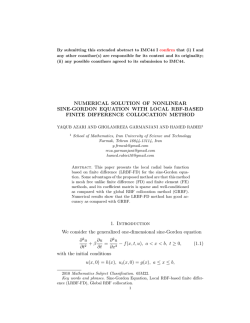
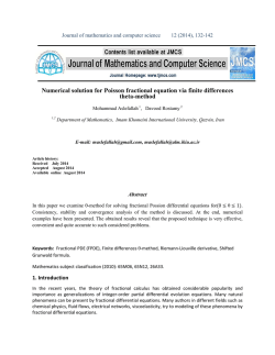
Journal of mathematics and computer science
13 (2014), 14-25
A nonlinear partial integro-differential equation arising in population dynamic
via radial basis functions and theta-method
Mohammad Aslefallah 1,2 and
1
Elyas Shivanian 1
Department of Mathematics, Imam Khomeini International University, Qazvin, Iran
2
Department of Mathematics, Karaj Branch, Islamic Azad University, Karaj, Iran
[email protected] , [email protected]
Article history:
Received July 2014
Accepted August 2014
Available online September 2014
Abstract
This paper proposes a numerical method to deal with the integro-differential reaction-diffusion
equation. In the proposed method, the time variable is eliminated by using finite difference рќњѓ в€’ method to
enjoy the stability condition. The method benefits from collocation radial basis function method, the
generallized thin plate splines (GTPS) radial basis functions are used. Therefore, it does not require any
struggle to determine shape parameter. The obtained results for some numerical examples reveal that the
proposed technique is very effective, convenient and quite accurate to such considered problems.
Keywords: Integro-differential equation, Radial basis functions, Kansa method, Finite
differences рќњѓ в€’ method.
2010 Mathematics subject classification: 34A08,35R11,65M06.
1 Introduction
Many problems in science and engineering modelled as differential equations. Solving
equations by traditional numerical methods such as finite difference (FDM), finite element (FEM) needs
generation of a regular mesh in the domain of the problem which is computationally expensive
[1,2,3,4,5]. During the last decade, meshless methods have received much attention. Due to the
difficulty of the mesh generation problem, meshless methods for simulation of the numerical problems
M. Aslefallah, E. Shivanian / J. Math. Computer Sci. 13 (2014), 14-25
are employed. Radial basis functions (RBFs) interpolation is a technique for representing a function
starting with data on scattered points [6,7,8,9]. The RBFs can be of various types, such as: polynomials of
a given degree; linear, quadratic, cubic, etc; thin plate spline (TPS), multiquadrics (MQ), inverse
multiquadrics (IMQ), Gaussian forms (GA), etc. Most differential equations do not have exact analytic
solutions, so approximation and numerical techniques must be used.
Development of constructive methods for the numerical solution of mathematical problems is a
main branch of mathematics. Meshless methods have attracted much attention in the both
mathematics and engineering community, recently. Extensive developments have been made in several
varieties of meshless techniques and applied to many applications in science and engineering. These
methods exist under different names, such as: the diffuse element method (DEM) [10], the hp-cloud
method [11], Meshless Local Petrov- Galerkin (MLPG) method [12,13,14], the meshless local boundary
integral equation (LBIE) method [15], the partition of unity method (PUM) [16], the meshless collocation
method based on radial basis functions (RBFs)[17], the smooth particle hydrodynamics (SPH)[19], the
reproducing kernel particle method (RKPM) [20], the radial point interpolation method [22], meshless
local radial point interpolation method (MLRPI) [23,24], and so on.
In this study, we implement the meshless collocation method for solving the following integrodifferential reaction-diffusion equation (also arising in population dynamic) [25,26] by using a radial
basis function (RBF):
∂𝑢(𝑥,𝑡)
∂𝑡
=
∂ 2 𝑢(𝑥,𝑡)
∂𝑥 2
+ рќ›Ѕрќ‘ў(1 в€’ рќ‘Ћрќ‘ў в€’ рќ‘ЏрќђЅ(рќ‘Ґ, рќ‘Ў)) + рќ‘“(рќ‘Ґ, рќ‘Ў),
(1)
where:
рќђЅ(рќ‘Ґ, рќ‘Ў) =
рќ‘Ґрќ‘…
‍𝜓(𝑥
рќ‘Ґрќђї
− 𝑦)𝑢(𝑦, 𝑡)𝑑𝑦
(for 𝑡 ∈ [0, 𝑇]) on a finite domain 𝑥𝐿 < 𝑥 < 𝑥𝑅 . 𝜓(𝑥) is kernel function and 𝑓(𝑥, 𝑡) is a given smooth
function.
Initial condition рќ‘ў(рќ‘Ґ, 0) = рќ‘”(рќ‘Ґ) for
рќ‘ў(рќ‘Ґрќђї , рќ‘Ў) = 0 and рќ‘ў(рќ‘Ґрќ‘… , рќ‘Ў) = 0.
рќ‘Ґрќђї < рќ‘Ґ < рќ‘Ґрќ‘… and boundary conditions are as follows:
In the special case, if 𝑏 = 0 and 𝑓(𝑥, 𝑡) = 0 we have well-known‍Fisher’s‍equation‍as:‍
∂𝑢(𝑥,𝑡)
∂𝑡
=
∂ 2 𝑢(𝑥,𝑡)
∂𝑥 2
+ рќ›Ѕрќ‘ў(1 в€’ рќ‘Ћрќ‘ў),
2 Preliminaries
For implementation of this method we need the following definitions.
Definition 2.1 ( Radial basis functions.) Considering a finite set of interpolation points
𝑋 = {𝑥1 , 𝑥2 , … , 𝑥𝑀 } ⊆ 𝑅 𝑑 and a function 𝑢: 𝑋 → 𝑅 𝑑 , according to the process of interpolation using
radial basis functions [6], the interpolant of u is constructed in the following form:
15
M. Aslefallah, E. Shivanian / J. Math. Computer Sci. 13 (2014), 14-25
(𝑆𝑢)(𝑥) =
рќ‘Ђ
𝑖=1 ‍𝜆𝑖 𝜑(∥
𝑥 − 𝑥𝑖 ∥) + 𝑝(𝑥), 𝑥 ∈ 𝑅 𝑑
where ∥. ∥ is the Euclidean norm and 𝜑(∥. ∥) is a radial function. Also, 𝑝(𝑥) is a linear combination of
polynomials on рќ‘… рќ‘‘ of total degree at most рќ‘љ в€’ 1 as follows:
рќ‘ќ(рќ‘Ґ) =
рќ‘Ђ+рќ‘™
𝑗 =𝑀+1 ‍𝜆𝑗 𝑞𝑗 (𝑥),
+рќ‘‘в€’1
рќ‘™ = (рќ‘љ
)
рќ‘‘
Moreover, the interpolant 𝑆𝑢 and additional conditions must be determined to satisfy the system:
(𝑆𝑢)(𝑥𝑖 ) = 𝑢(𝑥𝑖 )
рќ‘Ђ
𝑖=1 ‍𝜆𝑖 𝑞𝑗 (𝑥𝑖 ) = 0,
, 𝑖 = 1,2, … , 𝑀
рќ‘‘
, в€Ђрќ‘ћрќ‘— в€€ О рќ‘љ
в€’1
рќ‘‘
рќ‘‘
where О рќ‘љ
в€’1 denotes the space of all polynomials on рќ‘… of total degree at most рќ‘љ в€’ 1. Now we have a
unique interpolant (𝑆𝑢) of u if 𝜑(𝑟) is a conditionally positive definite radial basis function of order
m[28]. For any partial differential operator рќђї, рќђїрќ‘ў can be represented by:
рќђїрќ‘ў(рќ‘Ґ) =
𝑥 𝑖 ∈𝑋 ‍𝜆𝑖 𝐿𝜑(∥
𝑥 − 𝑥𝑖 ∥) + 𝐿𝑝(𝑥),
The coefficients рќњ†рќ‘– will be obtained by solving the system of linear equations.
We will use some RBFs which have the following form:
𝜑(∥ 𝑥 − 𝑥𝑖 ∥) = 𝜑(𝑟𝑖 )
Some types of RBFs presented in Table.1. (c is shape parameter)
Table 1. Some types of RBF functions
Name
Cubic
Thin plate splines
Generalized Thin plate splines
Inverse quadrics(or Cauchy)
Abbreviation
CU
TPS
GTPS
IQ
Multiquadrics
Inverse Multiquadrics
MQ
IMQ
Gaussian RBF
GA
Formula
рќњ‘(рќ‘џ) = рќ‘џ 3
рќњ‘(рќ‘џ) = рќ‘џ 2 log(рќ‘џ)
рќњ‘(рќ‘џ) = рќ‘џ 2рќ‘љ log(рќ‘џ), рќ‘љ в€€ рќ‘Ѓ
1
рќњ‘(рќ‘џ) = 2 2
рќњ‘(рќ‘џ) =
рќњ‘(рќ‘џ) =
рќ‘ђ +рќ‘џ
рќ‘ђ2 +
рќњ‘(рќ‘џ) = рќ‘’
1
рќ‘џ2
рќ‘ђ 2 +рќ‘џ 2
в€’рќ‘џ 2 /рќ‘ђ 2
Definition 2.2 𝜃 -method, (0 ≤ 𝜃 ≤ 1), is general finite-difference approximation to
рќњ• 2 рќ‘ў(рќ‘Ґ,рќ‘Ў)
рќњ•рќ‘Ґ 2
given by:
∂ 2 𝑢(𝑥,𝑡)
∂𝑥 2
в‰… рќњѓрќ›ї2,рќ‘Ґ рќ‘€рќ‘–,рќ‘— +1 + (1 в€’ рќњѓ)рќ›ї2,рќ‘Ґ рќ‘€рќ‘–,рќ‘— ,
such that we define:
16
(2)
M. Aslefallah, E. Shivanian / J. Math. Computer Sci. 13 (2014), 14-25
∇2 = 𝛿2,𝑥 𝑈𝑖,𝑗 =
(where рќ‘• = О”рќ‘Ґ =
рќ‘Ґ рќ‘… в€’рќ‘Ґ рќђї
рќ‘Ђ
1
(рќ‘€рќ‘–+1,рќ‘—
(О”рќ‘Ґ)2
в€’ 2рќ‘€рќ‘–,рќ‘— + рќ‘€рќ‘–в€’1,рќ‘— ),
рќ‘—
for рќ‘Ґ-axis and рќ‘€рќ‘–,рќ‘— = рќ‘€рќ‘– = рќ‘€(рќ‘Ґрќ‘– , рќ‘Ўрќ‘— ) represent the numerical approximation
solution) In other words:
∂ 2 𝑢(𝑥,𝑡)
∂𝑥 2
в‰…
1
(О”рќ‘Ґ)2
рќњѓ(рќ‘€рќ‘–+1,рќ‘— +1 в€’ 2рќ‘€рќ‘–,рќ‘— +1 + рќ‘€рќ‘–в€’1,рќ‘— +1 ) + (1 в€’ рќњѓ)(рќ‘€рќ‘–+1,рќ‘— в€’ 2рќ‘€рќ‘–,рќ‘— + рќ‘€рќ‘–в€’1,рќ‘— ) ,
1
Remark 2.3 Note that рќњѓ = 0 gives the explicit scheme, рќњѓ = 2 the Crank-Nicolson, and рќњѓ = 1 a fully
implicit backward time-difference method.
Remark 2.4 The laplacian operator рќ›» 2 for рќњ‘ function is given by
∇2 (𝜑(𝑟)) =
∂𝜑 ∂ 2 𝑟
∂ 2 𝜑 ∂𝑟 2
(
)
+
( ) ,
2
∂𝑟 ∂𝑥
∂𝑟 2 ∂𝑥
(3)
3 Discretization
According to definitions (2.1)and (2.2), from (1) and рќњѓ-method we get:
∂𝑢(𝑥,𝑡 𝑛 +1 )
∂𝑡
= [𝜃∇2 𝑢𝑛+1 + (1 − 𝜃)∇2 𝑢𝑛 ] + 𝛽𝑢𝑛+1 − 𝑎𝛽(𝑢𝑛 )2 − 𝑏𝛽𝑢𝑛 𝐽𝑛 + 𝑓 𝑛+1 ,
(4)
By substituting finite difference for left hand into (4) we have:
рќ‘ў рќ‘› +1 в€’рќ‘ў рќ‘›
О”рќ‘Ў
= [𝜃∇2 𝑢𝑛+1 + (1 − 𝜃)∇2 𝑢𝑛 ] + 𝛽𝑢𝑛+1 − 𝑎𝛽(𝑢𝑛 )2 − 𝑏𝛽𝑢𝑛 𝐽𝑛 + 𝑓 𝑛+1 ,
(5)
and for Δ𝑡 = �:
𝑢𝑛+1 − �𝜃∇2 𝑢𝑛+1 − �𝛽𝑢𝑛+1 = 𝑢𝑛 + �(1 − 𝜃)∇2 𝑢𝑛 − �𝑎𝛽(𝑢𝑛 )2 − �𝑏𝛽𝑢𝑛 𝐽𝑛 + �𝑓 𝑛+1 ,
(6)
In other words, we get:
(1 − �𝜃∇2 − �𝛽)𝑢𝑖𝑛+1 = 𝑢𝑖𝑛 + �(1 − 𝜃)∇2 𝑢𝑖𝑛 − �𝑎𝛽(𝑢𝑖𝑛 )2 − �𝑏𝛽𝑢𝑖𝑛 𝐽𝑖𝑛 + �𝑓𝑖𝑛+1 ,
(7)
Now, according to the mentioned method in one-dimensional case, if we collocate рќ‘Ђ different
points 𝑥1 , 𝑥2 , … , 𝑥𝑀 , then:
рќ‘ў(рќ‘Ґрќ‘– , рќ‘Ўрќ‘›+1 ) =
рќ‘Ђ
рќ‘›+1
𝜑(∥
𝑗 =1 ‍𝜆𝑗
рќ‘›+1
𝑥𝑖 − 𝑥𝑗 ∥) + 𝜆𝑛+1
рќ‘Ђ+1 рќ‘Ґрќ‘– + рќњ†рќ‘Ђ+2 ,
(8)
рќ‘Ђ
рќ‘›+1
рќ‘Ґрќ‘–
𝑗 =1 ‍𝜆𝑗
(9)
Two additional conditions can be described as:
рќ‘Ђ
рќ‘›+1
𝑗 =1 ‍𝜆𝑗
=
Finally, by combining equations (8),(9), we obtain a matrix form:
[рќ‘ў]рќ‘›+1 = рќђґ[рќњ†]рќ‘›+1
17
= 0,
M. Aslefallah, E. Shivanian / J. Math. Computer Sci. 13 (2014), 14-25
рќ‘›+1
where: [𝑢]𝑛+1 = [𝑢1𝑛+1 , 𝑢2𝑛+1 , … , 𝑢𝑀
, 0,0]𝑇
,
𝑛+1 𝑇
[рќњ†]рќ‘›+1 = [рќњ†1рќ‘›+1 , рќњ†рќ‘›+1
2 , … , 𝜆𝑀+2 ]
and the matrix рќђґ = (рќ‘Ћрќ‘–рќ‘— )(рќ‘Ђ+2)Г—(рќ‘Ђ+2) is given by:
рќњ‘11
в‹®
рќњ‘рќ‘–1
в‹®
рќђґ=
рќњ‘рќ‘Ђ1
рќ‘Ґ1
1
в‹Ї
в‹±
в‹Ї
в‹±
в‹Ї
в‹Ї
в‹Ї
рќњ‘1рќ‘—
в‹®
рќњ‘рќ‘–рќ‘—
в‹®
рќњ‘рќ‘Ђрќ‘—
рќ‘Ґрќ‘—
1
в‹Ї
в‹±
в‹Ї
в‹±
в‹Ї
в‹Ї
в‹Ї
рќњ‘1рќ‘Ђ
в‹®
рќњ‘рќ‘–рќ‘Ђ
в‹®
рќњ‘рќ‘Ђрќ‘Ђ
рќ‘Ґрќ‘Ђ
1
рќ‘Ґ1
в‹®
рќ‘Ґрќ‘–
в‹®
рќ‘Ґрќ‘Ђ
0
0
1
в‹®
1
в‹®
1
0
0
(10)
By substituting (8) into (5),(6) and considering (9) and initial and boundary conditions we obtain a
matrix form:
[рќ‘ђ]рќ‘›+1 = рќђµ[рќњ†]рќ‘›+1
where:
рќ‘›+1
[𝑐]𝑛+1 = [𝑐1𝑛+1 , 𝑐2𝑛+1 , … , 𝑐𝑀
, 0,0]𝑇
рќђї(рќњ‘11 )
в‹®
рќђї(рќњ‘рќ‘–1 )
в‹®
рќђµ=
рќђї(рќњ‘рќ‘Ђ1 )
рќ‘Ґ1
1
в‹Ї
в‹±
в‹Ї
в‹±
в‹Ї
в‹Ї
в‹Ї
(11)
and
рќђї(рќњ‘1рќ‘— )
в‹®
рќђї(рќњ‘рќ‘–рќ‘— )
в‹®
рќђї(рќњ‘рќ‘Ђрќ‘— )
рќ‘Ґрќ‘—
1
в‹Ї
в‹±
в‹Ї
в‹±
в‹Ї
в‹Ї
в‹Ї
рќђї(рќњ‘1рќ‘Ђ )
в‹®
рќђї(рќњ‘рќ‘–рќ‘Ђ )
в‹®
рќђї(рќњ‘рќ‘Ђрќ‘Ђ )
рќ‘Ґрќ‘Ђ
1
рќђї(рќ‘Ґ1 )
в‹®
рќђї(рќ‘Ґрќ‘– )
в‹®
рќђї(рќ‘Ґрќ‘Ђ )
0
0
рќђї(1)
в‹®
рќђї(1)
в‹®
рќђї(1)
0
0
(12)
where L represents an operator given by
(1 − �𝜃∇2 − �𝛽)(∗),
рќђї(в€—) = (в€—),
1<рќ‘–<рќ‘Ђ
рќ‘– = 1 or рќ‘– = рќ‘Ђ
(13)
and
рќ‘ђрќ‘–рќ‘›+1
𝑢𝑛 + �(1 − 𝜃)∇2 𝑢𝑛 − �𝑎𝛽(𝑢𝑛 )2 − �𝑏𝛽𝐽𝑖𝑛 + �𝑓 𝑛+1 ,
= рќ‘”(рќ‘Ґрќ‘– , рќ‘Ўрќ‘›+1 ),
𝑛 ≥ 0,1 < 𝑖 < 𝑀
рќ‘– = 1 or рќ‘– = рќ‘Ђ
We use the Simpson method for approximation of the integral term. By solving the system (11) we find
(рќ‘Ђ + 2) unknowns рќњ†рќ‘—рќ‘›+1 then with (8) we approximate the value of u.
4 Numerical Examples
We use the generalized thin plate splines(GTPS) which have the following form:
18
M. Aslefallah, E. Shivanian / J. Math. Computer Sci. 13 (2014), 14-25
рќњ‘(рќ‘џ) = рќ‘џ 2рќ‘љ log(рќ‘џ),
рќ‘љв€€рќ‘Ѓ
Example 4.1 Consider (1) in the special case for рќ‘Ћ = рќ‘Џ = 0, рќ›Ѕ = в€’1 (as a linear example) :
∂𝑢(𝑥,𝑡)
∂𝑡
=
∂ 2 𝑢(𝑥,𝑡)
∂𝑥 2
в€’ рќ‘ў(рќ‘Ґ, рќ‘Ў) + рќ‘“(рќ‘Ґ, рќ‘Ў),
(for 𝑡 ∈ [0, 𝑇]) on a finite domain [0,2]. Initial condition 𝑢(𝑥, 0) = 𝑔(𝑥) = 0 and boundary conditions
are:
рќ‘ў(0, рќ‘Ў) = рќ‘ў(2, рќ‘Ў) = 0.
with an exact analytical solution:
рќ‘ў(рќ‘Ґ, рќ‘Ў) = рќ‘Ў 2 рќ‘Ґ(2 в€’ рќ‘Ґ).
0≤𝑥≤2
when:
рќ‘“(рќ‘Ґ, рќ‘Ў) = 2рќ‘Ўрќ‘Ґ(2 в€’ рќ‘Ґ) + рќ‘Ў 2 рќ‘Ґ(2 в€’ рќ‘Ґ) + 2рќ‘Ў 2 ,
For рќ‘љ = 4 in GTPS, the approximated solution and error functions shown in Fig. 1 verify the reliability of
presented method. The Root mean square(RMS) of error value for some different values of рќњѓ and M are
given in Table2.
Table 2. Root mean square(RMS) of Example 4.1 at time 𝑇 = 2.
рќњѓ
0.5
0.75
1
О”рќ‘Ў
0.10
0.05
0.02
0.01
0.10
0.05
0.02
0.01
0.10
0.05
0.02
0.01
M
10
20
50
100
10
20
50
100
10
20
50
100
19
RMS
3.2745 e-3
9.3012 e-4
2.2047 e-4
9.2689 e-5
2.1991 e-3
6.8368 e-4
1.9322 e-4
8.8321 e-5
1.2820 e-3
4.9447 e-4
1.7504 e-4
8.5429 e-5
M. Aslefallah, E. Shivanian / J. Math. Computer Sci. 13 (2014), 14-25
Figure 1. Comparison between exact and numerical solutions for the Example 4.1 with рќ‘Ђ = 50, рќњѓ = 0.5
Example 4.2 Consider (1) in the special case for рќ‘Ћ = 1, рќ‘Џ = 0, рќ›Ѕ = 1 (as a nonlinear example) :
∂𝑢(𝑥,𝑡)
∂𝑡
=
∂ 2 𝑢(𝑥,𝑡)
∂𝑥 2
+ рќ‘ў(1 в€’ рќ‘ў) + рќ‘“(рќ‘Ґ, рќ‘Ў),
(for 𝑡 ∈ [0, 𝑇]) on a finite domain [−1,1]. Initial condition 𝑢(𝑥, 0) = 𝑔(𝑥) = (1 − 𝑥 4 )𝑠𝑖𝑛(𝑥) and
boundary conditions are:
рќ‘ў(в€’1, рќ‘Ў) = рќ‘ў(1, рќ‘Ў) = 0.
with an exact analytical solution:
рќ‘ў(рќ‘Ґ, рќ‘Ў) = (1 в€’ рќ‘Ґ 4 )рќ‘ рќ‘–рќ‘›(рќ‘Ґ + рќ‘Ў) .
−1≤𝑥 ≤1
when:
рќ‘“(рќ‘Ґ, рќ‘Ў) = (1 + 8рќ‘Ґ 3 в€’ рќ‘Ґ 4 )рќ‘ђрќ‘њрќ‘ (рќ‘Ґ + рќ‘Ў) + 12рќ‘Ґ 2 рќ‘ рќ‘–рќ‘›(рќ‘Ґ + рќ‘Ў) + (1 в€’ рќ‘Ґ 4 )2 рќ‘ рќ‘–рќ‘›2 (рќ‘Ґ + рќ‘Ў),
For рќ‘љ = 4 in GTPS, the approximated solution and error functions shown in Fig. 2 verify the reliability of
presented method. The Root mean square(RMS) of error value for some different values of рќњѓ and M are
given in Table3.
20
M. Aslefallah, E. Shivanian / J. Math. Computer Sci. 13 (2014), 14-25
Table 3. Root mean square(RMS) of Example 4.2 at time 𝑇 = 2.
рќњѓ
0.5
О”рќ‘Ў
0.10
0.05
0.02
0.01
0.10
0.05
0.02
0.01
0.10
0.05
0.02
0.01
M
10
20
50
100
10
20
50
100
10
20
50
100
0.75
1
RMS
1.7312 e-3
4.7132 e-4
9.1033 e-5
3.1253 e-5
9.9762 e-4
2.8700 e-4
6.5481 e-5
2.6401 e-5
5.1844 e-4
1.6413 e-4
4.9833 e-5
2.3557 e-5
Figure 2. Comparison between exact and numerical solutions for the Example 4.2 with рќ‘Ђ = 50, рќњѓ = 0.5
Example 4.3 Consider (1) for рќ‘Ћ = 1, рќ‘Џ = 1, рќ›Ѕ = 1 (as a nonlinear integro-differential example) :
∂𝑢(𝑥,𝑡)
∂𝑡
=
∂ 2 𝑢(𝑥,𝑡)
∂𝑥 2
+ рќ‘ў(1 в€’ рќ‘ў в€’ рќђЅ(рќ‘Ґ, рќ‘Ў)) + рќ‘“(рќ‘Ґ, рќ‘Ў),
(for 𝑡 ∈ [0, 𝑇]) on a finite domain [−1,1].
Where:
21
M. Aslefallah, E. Shivanian / J. Math. Computer Sci. 13 (2014), 14-25
рќђЅ(рќ‘Ґ, рќ‘Ў) =
1
‍𝑒 𝑥−𝑦 𝑢(𝑦, 𝑡)𝑑𝑦,
в€’1
Initial condition рќ‘ў(рќ‘Ґ, 0) = рќ‘”(рќ‘Ґ) = рќ‘ рќ‘–рќ‘›(2рќњ‹рќ‘Ґ) and boundary conditions are:
рќ‘ў(в€’1, рќ‘Ў) = рќ‘ў(1, рќ‘Ў) = 0.
with an exact analytical solution:
рќ‘ў(рќ‘Ґ, рќ‘Ў) = (1 в€’ рќ‘Ґ 4 )рќ‘ рќ‘–рќ‘›(рќ‘Ґ + рќ‘Ў) .
−1≤𝑥 ≤1
when:
рќ‘“(рќ‘Ґ, рќ‘Ў) = рќ‘ў(рќ‘Ґ, рќ‘Ў)рќђЅ(рќ‘Ґ, рќ‘Ў) + рќ‘•(рќ‘Ґ, рќ‘Ў),
and:
рќ‘•(рќ‘Ґ, рќ‘Ў) = (1 + 8рќ‘Ґ 3 в€’ рќ‘Ґ 4 )рќ‘ђрќ‘њрќ‘ (рќ‘Ґ + рќ‘Ў) + 12рќ‘Ґ 2 рќ‘ рќ‘–рќ‘›(рќ‘Ґ + рќ‘Ў) + (1 в€’ рќ‘Ґ 4 )2 рќ‘ рќ‘–рќ‘›2 (рќ‘Ґ + рќ‘Ў),
For рќ‘љ = 3 in GTPS, the approximated solution and error functions shown in Fig. 3 verify the reliability of
presented method. The Root mean square(RMS) of error value for some different values of рќњѓ and M are
given in Table4.
Table 4. Root mean square(RMS) of Example 4.3 at time 𝑇 = 2.
рќњѓ
0.5
0.75
1
О”рќ‘Ў
0.10
0.05
0.02
0.01
0.10
0.05
0.02
0.01
0.10
0.05
0.02
0.01
M
10
20
50
100
10
20
50
100
10
20
50
100
22
RMS
1.8278 e-3
6.2988 e-4
2.0270 e-4
9.7285 e-5
1.1707 e-3
5.0246 e-4
1.9135 e-4
9.5507 e-5
8.0165 e-4
4.3730 e-4
1.8530 e-4
9.4433 e-5
M. Aslefallah, E. Shivanian / J. Math. Computer Sci. 13 (2014), 14-25
Figure 3. Comparison between exact and numerical solutions for the Example 4.3 with рќ‘Ђ = 50, рќњѓ = 0.5
5 Conclusion
In this paper we have presented a numerical scheme based on combination of meshless
collocation radial basis function (so-called‍Kansa’s‍method) and 𝜃 −method. The 𝜃 −method has been
applied to derivative. The method has been tested on three illustrative numerical examples. The
computational results are found to be in good agreement with the exact solutions.
References
[1] L. Sabatelli, S. Keating, J. Dudley, P. Richmond: Waiting time distributions in financial
markets, European Physical Journal B, 27, (2002), 273-275.
[2] R. Schumer, D.A. Benson, M.M. Meerschaert, S.W. Wheatcraft: Eulerian derivation of the
fractional advection-dispersion equation, Journal of Contaminant Hydrology, 48, (2001), 69-88.
[3] R. Hilfer: Applications of Fractional Calculus in Physics, World Scientific, Singapore. (2000)
23
M. Aslefallah, E. Shivanian / J. Math. Computer Sci. 13 (2014), 14-25
[4] M.M. Meerschaert, C. Tadjeran: Finite Difference Approximations for two-sided spacefractional partial differential equations, Applied Numerical Mathematics, 56, (2006), 80-90.
[5]
S. Samko, A. Kibas, O. Marichev: Fractional Integrals and derivatives: Theory and
Applications, Gordon and Breach, London. (1993)
[6] MD. Buhmann: Radial basis functions: theory and implementations. Cambridge University
Press. (2003)
[7] V.R. Hosseini, W. Chen, Z. Avazzadeh: Numerical solution of fractional telegraph equation by
using radial basis functions, Eng. Anal. Boundary. Elem. ,38, (2014), 31-39.
[8] S. Abbasbandy, H.R. Ghehsareh, I. Hashim: Numerical analysis of a mathematical model for
capillary formation in tumor angiogenesis using a meshfree method based on the radial basis function,
Eng. Anal. Boundary. Elem. 36(12), (2012), 1811-1818.
[9] S. Abbasbandy, H.R. Ghehsareh, I. Hashim: A meshfree method for the solution of twodimensional cubic nonlinear schrödinger equation, Eng. Anal. Boundary. Elem. 37(6), (2013), 885-898.
[10] B. Nayroles, G. Touzot, P. Villon: Generalizing the finite element method: diffuse
approximation and diffuse elements, Comput. Mech., 10, (1992), 307-318.
[11] C. Duarte, J. Oden: An h-p adaptative method using clouds, Comput. Methods Appl. Mech.
Engrg. 139, (1996), 237-262.
[12] S.N. Atluri, T.L. Zhu: A new meshless local Petrov-Galerkin (MLPG) approach in
computational mechanics, Comput. Mech. 22 (2), (1998), 117-127.
[13] S. Abbasbandy, V. Sladek, A. Shirzadi, J. Sladek: Numerical Simulations for Coupled Pair of
Diffusion Equations by MLPG Method, CMES Compt. Model. Eng. Sci. 71 (1), (2011), 15-37.
[14] A. Shirzadi, L. Ling, S. Abbasbandy: Meshless simulations of the two-dimensional fractionaltime convectiondiffusion- reaction equations, Eng. Anal. Bound. Elem. 36, (2012), 1522-1527.
[15] T. Zhu, J.D. Zhang, S.N. Atluri: A local boundary integral equation (LBIE) method in
computational mechanics and a meshless discretization approach, Comput. Mech. 21, (1998), 223-235.
[16] J.M. Melenk, I. Babuska: The partition of unity finite element method: basic theory and
applications, Comput. Methods Appl. Mech. Engrg. 139, (1996), 289-314.
[17] E.J. Kansa: Multiquadrics-a scattered data approximation scheme with applications to
computational fluid dynamics-II, J. Comput. Math. Appl. 19, (1990), 147-161.
[18] M. Aslefallah, D. Rostamy: A Numerical Scheme For Solving Space-Fractional Equation By
Finite Differences Theta-Method, Int. J. of Adv. in Aply. Math. and Mech., 1(4) , (2014),1-9.
[19] L.B. Lucy: A numerical approach to the testing of fusion process, Astron. J. 88, (1977),
1013-1024.
24
M. Aslefallah, E. Shivanian / J. Math. Computer Sci. 13 (2014), 14-25
[20] W.K. Liu, S. Jun, Y.F. Zhang: Reproducing kernel particle methods, Int. J. Numer. Methods
Fluids, 21, (1995), 1081-1106.
[21] M. Aslefallah, D. Rostamy, K. Hosseinkhani: Solving time-fractional differential diffusion
equation by theta-method, Int. J. of Adv. in Aply. Math. and Mech., 2(1) , (2014),1-8.
[22] G.R. Liu: Mesh Free Methods: Moving beyond the Finite Element Method, CRC Press.(2003)
[23] E. Shivanian: Analysis of meshless local radial point interpolation (MLRPI) on a nonlinear
partial integro-differential equation arising in population dynamics, Eng. Anal. Boundary. Elem. 37,
(2013), 1693-1702.
[24] M. Dehghan, A. Ghesmati: Numerical simulation of two-dimensional sine-gordon solitons
via a local weak meshless technique based on the radial point interpolation method (RPIM), Comput.
Phys. Commun. 181, (2010), 772-786.
[25] N. Apreutesei, N. Bessonov, V. Volpert, V. Vougalter: Spatial structures and generalized
travelling waves for an integro-differential equation, Discrete and Continuous Dynamical Systems Series
B, 13, (2010), 537-557.
[26] F. Fakhar-Izadi, M. Dehghan: An efficient pseudo-spectral LegendreGalerkin method for
solving a nonlinear partial integro-differential equation arising in population dynamics. Math. Methods
Appl. Sci. 36(12), (2013), 1485-1511.
[27] M. Aslefallah, D. Rostamy: Numerical solution for Poisson fractional equation via finite
differences theta-method, J. Math. Computer Sci. , TJMCS, 12(2) , (2014), 132-142.
[28] C.A. Micchell: Interpolation of scattered data; distance matrices and conditionally positive
definite functions, Constr. Approx., 2, (1986), 11-22.
25

Numerical Solutions of Huxley Equation By Haar Wavelet Method Ö

Abstract

裏表紙 - 大豊町

NUMERICAL SOLUTION OF NONLINEAR SINE - ResearchGate

数学と現象： - 宮崎大学 情報基盤センター

MATH 100 ELEMENTS OF FINITE MATHEMATICS

Vol12 Iss2 132-142 Numerical solution for Poisson frac

final program - INT

ASSOCIAZIONE NAZIONALE MECCANICA - GIMC

PSM Circular No. K of 2014

308, 2nd Floor, August Kranti Bhawan, Bhikaji Cama Place, New Delhi

Effective Virtual Teams for New Product Development

Rational Laguerre Functions and Their Applications - JMCS

13-30 - Global Science Press

Introduction to Metric and Topological Spaces by Wilson Sutherland

Catalog and Student Handbook - Chattahoochee Valley Community

Catalog and Student Handbook - Chattahoochee Valley Community

74-88 - Global Science Press

Chapter 33 Interference and Diffraction