QGIS User Guide
リリース 2.2
QGIS Project
2014 年 12 月 04 日
Contents
1 はじめに
3
2 記述ルール
2.1 GUI 記述ルール . . . . . . . . . . . . . . . . . . . . . . . . . . . . . . . . . . . . . . . . . . .
2.2 テキストやキーボードの記述ルール . . . . . . . . . . . . . . . . . . . . . . . . . . . . . . . .
2.3 プラットフォーム特有の操作方法 . . . . . . . . . . . . . . . . . . . . . . . . . . . . . . . . .
5
5
5
6
3 序文
7
4 特徴
4.1
4.2
4.3
4.4
4.5
4.6
4.7
4.8
5
.
.
.
.
.
.
.
.
.
.
.
.
.
.
.
.
.
.
.
.
.
.
.
.
.
.
.
.
.
.
.
.
.
.
.
.
.
.
.
.
.
.
.
.
.
.
.
.
.
.
.
.
.
.
.
.
.
.
.
.
.
.
.
.
.
.
.
.
.
.
.
.
.
.
.
.
.
.
.
.
.
.
.
.
.
.
.
.
.
.
.
.
.
.
.
.
.
.
.
.
.
.
.
.
.
.
.
.
.
.
.
.
.
.
.
.
.
.
.
.
.
.
.
.
.
.
.
.
.
.
.
.
.
.
.
.
.
.
.
.
.
.
.
.
.
.
.
.
.
.
.
.
.
.
.
.
.
.
.
.
.
.
.
.
.
.
.
.
.
.
.
.
.
.
.
.
.
.
.
.
.
.
.
.
.
.
.
.
.
.
.
.
.
.
.
.
.
.
.
.
.
.
.
.
.
.
.
.
.
.
.
.
.
.
.
.
9
9
9
10
10
10
11
11
12
What’s new in QGIS 2.2
5.1 アプリケーションとプロジェクトオプション
5.2 データプロバイダ . . . . . . . . . . . . . . . .
5.3 Digitising . . . . . . . . . . . . . . . . . . . . .
5.4 General . . . . . . . . . . . . . . . . . . . . . .
5.5 マップコンポーザ . . . . . . . . . . . . . . . .
5.6 QGIS サーバ . . . . . . . . . . . . . . . . . . .
5.7 シンボロジー . . . . . . . . . . . . . . . . . .
5.8 ユーザーインターフェース . . . . . . . . . . .
.
.
.
.
.
.
.
.
.
.
.
.
.
.
.
.
.
.
.
.
.
.
.
.
.
.
.
.
.
.
.
.
.
.
.
.
.
.
.
.
.
.
.
.
.
.
.
.
.
.
.
.
.
.
.
.
.
.
.
.
.
.
.
.
.
.
.
.
.
.
.
.
.
.
.
.
.
.
.
.
.
.
.
.
.
.
.
.
.
.
.
.
.
.
.
.
.
.
.
.
.
.
.
.
.
.
.
.
.
.
.
.
.
.
.
.
.
.
.
.
.
.
.
.
.
.
.
.
.
.
.
.
.
.
.
.
.
.
.
.
.
.
.
.
.
.
.
.
.
.
.
.
.
.
.
.
.
.
.
.
.
.
.
.
.
.
.
.
.
.
.
.
.
.
.
.
.
.
.
.
.
.
.
.
.
.
.
.
.
.
.
.
.
.
.
.
.
.
.
.
.
.
.
.
.
.
.
.
13
13
13
13
14
14
15
15
16
データを見る . . . . . . . . . . . . . . .
データの検索と表示地図の構成 . . . . .
データの作成、編集、管理と出力 . . . .
データ解析 . . . . . . . . . . . . . . . . .
インターネットへの地図公開 . . . . . .
プラグインを利用した QGIS 機能の拡張
Python コンソール . . . . . . . . . . . . .
既知の問題 . . . . . . . . . . . . . . . . .
6 はじめましょう
6.1 インストール . . . . . . .
6.2 サンプルデータ . . . . . .
6.3 サンプルセッション . . .
6.4 QGIS の起動と終了 . . . .
6.5 コマンドラインオプション
6.6 プロジェクト . . . . . . .
6.7 出力 . . . . . . . . . . . .
.
.
.
.
.
.
.
.
.
.
.
.
.
.
.
.
.
.
.
.
.
.
.
.
.
.
.
.
.
.
.
.
.
.
.
.
.
.
.
.
.
.
.
.
.
.
.
.
.
.
.
.
.
.
.
.
.
.
.
.
.
.
.
.
.
.
.
.
.
.
.
.
.
.
.
.
.
.
.
.
.
.
.
.
.
.
.
.
.
.
.
.
.
.
.
.
.
.
.
.
.
.
.
.
.
.
.
.
.
.
.
.
.
.
.
.
.
.
.
.
.
.
.
.
.
.
.
.
.
.
.
.
.
.
.
.
.
.
.
.
.
.
.
.
.
.
.
.
.
.
.
.
.
.
.
.
.
.
.
.
.
.
.
.
.
.
.
.
.
.
.
.
.
.
.
.
.
.
.
.
.
.
.
.
.
.
.
.
.
.
.
.
.
.
.
.
.
.
.
.
.
.
.
.
.
.
.
.
.
.
.
.
.
.
.
.
.
.
.
.
.
.
.
.
.
.
.
.
.
.
.
.
.
.
.
.
.
.
.
.
.
.
.
.
.
.
.
.
.
.
.
.
.
.
.
.
.
.
.
.
.
.
.
.
.
.
.
.
.
.
.
.
.
.
.
17
17
17
18
19
19
21
22
.
.
.
.
.
.
.
.
.
.
.
.
.
.
.
.
.
.
.
.
.
.
.
.
.
.
.
.
.
.
.
.
.
.
.
.
.
.
.
.
.
.
.
.
.
.
.
.
.
.
.
.
.
.
.
.
.
.
.
.
.
.
.
.
.
.
.
.
.
.
.
.
.
.
.
.
.
.
.
.
.
.
.
.
.
.
.
.
.
.
.
.
.
.
.
.
.
.
.
.
.
.
.
.
.
.
.
.
.
.
.
.
.
.
.
.
.
.
.
.
.
.
.
.
.
.
.
.
.
.
.
.
.
.
.
.
.
.
.
.
.
.
.
.
.
.
.
.
.
.
.
.
.
.
.
.
.
.
.
.
.
.
.
.
.
.
.
.
.
.
.
.
.
.
.
.
.
.
.
.
.
.
.
.
.
23
24
29
29
31
32
8 一般ツール
8.1 キーボードショートカット . . . . . . . . . . . . . . . . . . . . . . . . . . . . . . . . . . . . .
33
33
7
QGIS GUI
7.1 メニューバー .
7.2 ツールバー . . .
7.3 地図凡例 . . . .
7.4 地図ビュー . . .
7.5 ステータスバー
.
.
.
.
.
.
.
.
.
.
.
.
.
.
.
.
.
.
.
.
.
.
.
.
.
.
.
.
.
.
i
8.2
8.3
8.4
8.5
8.6
8.7
8.8
8.9
コンテキストヘルプ .
レンダリング . . . . .
計測 . . . . . . . . . .
地物情報表示 . . . . .
整飾 . . . . . . . . . .
アノテーションツール
空間ブックマーク . . .
プロジェクトの入れ子
.
.
.
.
.
.
.
.
.
.
.
.
.
.
.
.
.
.
.
.
.
.
.
.
.
.
.
.
.
.
.
.
.
.
.
.
.
.
.
.
.
.
.
.
.
.
.
.
.
.
.
.
.
.
.
.
.
.
.
.
.
.
.
.
.
.
.
.
.
.
.
.
.
.
.
.
.
.
.
.
.
.
.
.
.
.
.
.
.
.
.
.
.
.
.
.
.
.
.
.
.
.
.
.
.
.
.
.
.
.
.
.
.
.
.
.
.
.
.
.
.
.
.
.
.
.
.
.
.
.
.
.
.
.
.
.
.
.
.
.
.
.
.
.
.
.
.
.
.
.
.
.
.
.
.
.
.
.
.
.
.
.
.
.
.
.
.
.
.
.
.
.
.
.
.
.
.
.
.
.
.
.
.
.
.
.
.
.
.
.
.
.
.
.
.
.
.
.
.
.
.
.
.
.
.
.
.
.
.
.
.
.
.
.
.
.
.
.
.
.
.
.
.
.
.
.
.
.
.
.
.
.
.
.
.
.
.
.
.
.
.
.
.
.
.
.
.
.
.
.
.
.
.
.
.
.
.
.
.
.
.
.
.
.
.
.
.
.
.
.
.
.
.
.
.
.
.
.
.
.
.
.
.
.
.
.
.
.
.
.
.
.
.
.
.
.
.
.
.
.
.
.
.
.
33
34
35
37
38
41
42
43
QGIS 設定
9.1 パネルとツールバー . . .
9.2 プロジェクトのプロパティ
9.3 オプション . . . . . . . . .
9.4 カスタマイゼーション . .
.
.
.
.
.
.
.
.
.
.
.
.
.
.
.
.
.
.
.
.
.
.
.
.
.
.
.
.
.
.
.
.
.
.
.
.
.
.
.
.
.
.
.
.
.
.
.
.
.
.
.
.
.
.
.
.
.
.
.
.
.
.
.
.
.
.
.
.
.
.
.
.
.
.
.
.
.
.
.
.
.
.
.
.
.
.
.
.
.
.
.
.
.
.
.
.
.
.
.
.
.
.
.
.
.
.
.
.
.
.
.
.
.
.
.
.
.
.
.
.
.
.
.
.
.
.
.
.
.
.
.
.
.
.
.
.
.
.
.
.
.
.
.
.
.
.
.
.
45
45
46
46
54
10 投影法の利用方法
10.1 投影法サポート概要 . . . . . . . . . .
10.2 グローバル投影法指定 . . . . . . . . .
10.3 オンザフライ再投影 (OTF) を定義する
10.4 カスタム空間参照システム . . . . . . .
10.5 デフォルト datum 変換 . . . . . . . . .
.
.
.
.
.
.
.
.
.
.
.
.
.
.
.
.
.
.
.
.
.
.
.
.
.
.
.
.
.
.
.
.
.
.
.
.
.
.
.
.
.
.
.
.
.
.
.
.
.
.
.
.
.
.
.
.
.
.
.
.
.
.
.
.
.
.
.
.
.
.
.
.
.
.
.
.
.
.
.
.
.
.
.
.
.
.
.
.
.
.
.
.
.
.
.
.
.
.
.
.
.
.
.
.
.
.
.
.
.
.
.
.
.
.
.
.
.
.
.
.
.
.
.
.
.
.
.
.
.
.
.
.
.
.
.
.
.
.
.
.
.
.
.
.
.
.
.
.
.
.
55
55
55
57
58
59
9
.
.
.
.
.
.
.
.
11 QGIS ブラウザ
12 ベクタデータの操作
12.1 サポートされるデータ形式 . .
12.2 ベクタプロパティダイアログ
12.3 編集 . . . . . . . . . . . . . .
12.4 クエリビルダー . . . . . . . .
12.5 フィールド計算機 . . . . . . .
61
.
.
.
.
.
.
.
.
.
.
.
.
.
.
.
.
.
.
.
.
.
.
.
.
.
.
.
.
.
.
.
.
.
.
.
.
.
.
.
.
.
.
.
.
.
.
.
.
.
.
.
.
.
.
.
.
.
.
.
.
.
.
.
.
.
.
.
.
.
.
.
.
.
.
.
.
.
.
.
.
.
.
.
.
.
.
.
.
.
.
.
.
.
.
.
.
.
.
.
.
.
.
.
.
.
.
.
.
.
.
.
.
.
.
.
.
.
.
.
.
.
.
.
.
.
.
.
.
.
.
.
.
.
.
.
.
.
.
.
.
.
.
.
.
.
.
.
.
.
.
.
.
.
.
.
.
.
.
.
.
.
.
.
.
.
.
.
.
.
.
63
. 63
. 76
. 103
. 120
. 121
13 ラスタデータの操作
127
13.1 ラスターデータの操作 . . . . . . . . . . . . . . . . . . . . . . . . . . . . . . . . . . . . . . . 127
13.2 ラスタのプロパティダイアログ . . . . . . . . . . . . . . . . . . . . . . . . . . . . . . . . . . 128
13.3 ラスタ計算機 . . . . . . . . . . . . . . . . . . . . . . . . . . . . . . . . . . . . . . . . . . . . 135
14 OGC データの操作
139
14.1 OGC データクライアントとしての QGIS . . . . . . . . . . . . . . . . . . . . . . . . . . . . . 139
14.2 OGC データサーバとしての QGIS . . . . . . . . . . . . . . . . . . . . . . . . . . . . . . . . . 148
15 GPS データの操作
153
15.1 GPS プラグイン . . . . . . . . . . . . . . . . . . . . . . . . . . . . . . . . . . . . . . . . . . . 153
15.2 Live GPS トラッキング . . . . . . . . . . . . . . . . . . . . . . . . . . . . . . . . . . . . . . . 157
16 GRASS GIS の統合
16.1 GRASS プラグインの起動 . . . . . . . . . . .
16.2 GRASS ラスタとベクタレイヤのロード . . .
16.3 GRASS LOCATION と MAPSET . . . . . . . .
16.4 GRASS LOCATION へデータをインポート . .
16.5 GRASS ベクターデータモデル . . . . . . . . .
16.6 新しい GRASS ベクターレイヤーの作成 . . .
16.7 GRASS ベクタレイヤのデジタイジングと編集
16.8 GRASS 領域ツール . . . . . . . . . . . . . . .
16.9 GRASS ツールボックス . . . . . . . . . . . .
.
.
.
.
.
.
.
.
.
.
.
.
.
.
.
.
.
.
.
.
.
.
.
.
.
.
.
.
.
.
.
.
.
.
.
.
.
.
.
.
.
.
.
.
.
.
.
.
.
.
.
.
.
.
.
.
.
.
.
.
.
.
.
.
.
.
.
.
.
.
.
.
.
.
.
.
.
.
.
.
.
.
.
.
.
.
.
.
.
.
.
.
.
.
.
.
.
.
.
.
.
.
.
.
.
.
.
.
.
.
.
.
.
.
.
.
.
.
.
.
.
.
.
.
.
.
.
.
.
.
.
.
.
.
.
.
.
.
.
.
.
.
.
.
.
.
.
.
.
.
.
.
.
.
.
.
.
.
.
.
.
.
.
.
.
.
.
.
.
.
.
.
.
.
.
.
.
.
.
.
.
.
.
.
.
.
.
.
.
.
.
.
.
.
.
.
.
.
.
.
.
.
.
.
.
.
.
.
.
.
.
.
.
.
.
.
.
.
.
.
.
.
.
.
.
.
.
.
.
.
.
.
.
.
163
163
164
164
167
167
168
168
171
171
17 QGIS プロセッシングフレームワーク
17.1 はじめに . . . . . . . . . . . . . . . .
17.2 ツールボックス . . . . . . . . . . . .
17.3 グラフィカルモデラー . . . . . . . .
17.4 バッチプロセシングインタフェース .
.
.
.
.
.
.
.
.
.
.
.
.
.
.
.
.
.
.
.
.
.
.
.
.
.
.
.
.
.
.
.
.
.
.
.
.
.
.
.
.
.
.
.
.
.
.
.
.
.
.
.
.
.
.
.
.
.
.
.
.
.
.
.
.
.
.
.
.
.
.
.
.
.
.
.
.
.
.
.
.
.
.
.
.
.
.
.
.
.
.
.
.
.
.
.
.
.
.
.
.
.
.
.
.
181
181
182
191
197
ii
.
.
.
.
.
.
.
.
.
.
.
.
.
.
.
.
.
.
.
.
17.5
17.6
17.7
17.8
処理アルゴリズムをコンソールから使う
履歴マネージャ . . . . . . . . . . . . . .
外部アプリケーションの設定 . . . . . .
The SEXTANTE Commander . . . . . . .
18 プリントコンポーザ
18.1 最初のステップ . . . . .
18.2 レンダリングモード . .
18.3 コンポーザアイテム . .
18.4 アイテムの管理 . . . . .
18.5 取り消しと再実行ツール
18.6 地図帳の生成 . . . . . .
18.7 出力の作成 . . . . . . . .
18.8 コンポーザの管理 . . . .
.
.
.
.
.
.
.
.
.
.
.
.
.
.
.
.
.
.
.
.
.
.
.
.
.
.
.
.
.
.
.
.
.
.
.
.
.
.
.
.
.
.
.
.
.
.
.
.
.
.
.
.
.
.
.
.
.
.
.
.
.
.
.
.
.
.
.
.
.
.
.
.
.
.
.
.
.
.
.
.
.
.
.
.
.
.
.
.
.
.
.
.
.
.
.
.
.
.
.
.
.
.
.
.
.
.
.
.
.
.
.
.
.
.
.
.
199
204
205
212
.
.
.
.
.
.
.
.
.
.
.
.
.
.
.
.
.
.
.
.
.
.
.
.
.
.
.
.
.
.
.
.
.
.
.
.
.
.
.
.
.
.
.
.
.
.
.
.
.
.
.
.
.
.
.
.
.
.
.
.
.
.
.
.
.
.
.
.
.
.
.
.
.
.
.
.
.
.
.
.
.
.
.
.
.
.
.
.
.
.
.
.
.
.
.
.
.
.
.
.
.
.
.
.
.
.
.
.
.
.
.
.
.
.
.
.
.
.
.
.
.
.
.
.
.
.
.
.
.
.
.
.
.
.
.
.
.
.
.
.
.
.
.
.
.
.
.
.
.
.
.
.
.
.
.
.
.
.
.
.
.
.
.
.
.
.
.
.
.
.
.
.
.
.
.
.
.
.
.
.
.
.
.
.
.
.
.
.
.
.
.
.
.
.
.
.
.
.
.
.
.
.
.
.
.
.
.
.
.
.
.
.
.
.
.
.
.
.
.
.
.
.
.
.
.
.
.
.
.
.
.
.
.
.
.
.
.
.
.
.
.
.
.
.
.
.
.
.
.
.
.
.
.
.
.
.
.
.
.
.
.
.
.
.
215
217
220
221
235
237
237
239
240
19 プラグイン
19.1 QGIS プラグイン . . . . . . . . . .
19.2 QGIS コアプラグインを利用する .
19.3 座標取得プラグイン . . . . . . . .
19.4 DB マネージャプラグイン . . . . .
19.5 Dxf2Shp コンバータープラグイン .
19.6 eVis プラグイン . . . . . . . . . . .
19.7 fTools プラグイン . . . . . . . . . .
19.8 GDAL ツールズプラグイン . . . . .
19.9 ジオレファレンサプラグイン . . .
19.10 データ補間プラグイン . . . . . . .
19.11 オフライン編集プラグイン . . . . .
19.12 Oracle Spatial GeoRaster プラグイン
19.13 ラスター地形解析プラグイン . . .
19.14 ヒートマッププラグイン . . . . . .
19.15 道路グラフプラグイン . . . . . . .
19.16 空間検索プラグイン . . . . . . . .
19.17 SPIT プラグイン . . . . . . . . . . .
19.18 SQL Anywhere プラグイン . . . . .
19.19 トポロジチェッカープラグイン . .
19.20 地域統計プラグイン . . . . . . . .
.
.
.
.
.
.
.
.
.
.
.
.
.
.
.
.
.
.
.
.
.
.
.
.
.
.
.
.
.
.
.
.
.
.
.
.
.
.
.
.
.
.
.
.
.
.
.
.
.
.
.
.
.
.
.
.
.
.
.
.
.
.
.
.
.
.
.
.
.
.
.
.
.
.
.
.
.
.
.
.
.
.
.
.
.
.
.
.
.
.
.
.
.
.
.
.
.
.
.
.
.
.
.
.
.
.
.
.
.
.
.
.
.
.
.
.
.
.
.
.
.
.
.
.
.
.
.
.
.
.
.
.
.
.
.
.
.
.
.
.
.
.
.
.
.
.
.
.
.
.
.
.
.
.
.
.
.
.
.
.
.
.
.
.
.
.
.
.
.
.
.
.
.
.
.
.
.
.
.
.
.
.
.
.
.
.
.
.
.
.
.
.
.
.
.
.
.
.
.
.
.
.
.
.
.
.
.
.
.
.
.
.
.
.
.
.
.
.
.
.
.
.
.
.
.
.
.
.
.
.
.
.
.
.
.
.
.
.
.
.
.
.
.
.
.
.
.
.
.
.
.
.
.
.
.
.
.
.
.
.
.
.
.
.
.
.
.
.
.
.
.
.
.
.
.
.
.
.
.
.
.
.
.
.
.
.
.
.
.
.
.
.
.
.
.
.
.
.
.
.
.
.
.
.
.
.
.
.
.
.
.
.
.
.
.
.
.
.
.
.
.
.
.
.
.
.
.
.
.
.
.
.
.
.
.
.
.
.
.
.
.
.
.
.
.
.
.
.
.
.
.
.
.
.
.
.
.
.
.
.
.
.
.
.
.
.
.
.
.
.
.
.
.
.
.
.
.
.
.
.
.
.
.
.
.
.
.
.
.
.
.
.
.
.
.
.
.
.
.
.
.
.
.
.
.
.
.
.
.
.
.
.
.
.
.
.
.
.
.
.
.
.
.
.
.
.
.
.
.
.
.
.
.
.
.
.
.
.
.
.
.
.
.
.
.
.
.
.
.
.
.
.
.
.
.
.
.
.
.
.
.
.
.
.
.
.
.
.
.
.
.
.
.
.
.
.
.
.
.
.
.
.
.
.
.
.
.
.
.
.
.
.
.
.
.
.
.
.
.
.
.
.
.
.
.
.
.
.
.
.
.
.
.
.
.
.
.
.
.
.
.
.
.
.
.
.
.
.
.
.
.
.
.
.
.
.
.
.
.
.
.
.
.
.
.
.
.
.
.
.
.
.
.
.
.
.
.
.
.
.
.
.
.
.
.
.
.
.
.
.
.
.
.
.
.
.
.
.
.
.
.
.
.
.
.
.
.
.
.
.
.
.
.
.
.
.
.
.
.
.
.
.
.
.
.
.
.
.
.
.
.
.
.
.
.
.
.
.
.
.
.
.
.
.
.
.
.
.
.
.
.
.
.
.
.
.
.
.
.
.
243
243
247
248
248
249
250
259
263
266
270
271
272
274
275
277
280
281
283
283
286
20 ヘルプとサポート
20.1 メーリングリスト
20.2 IRC . . . . . . . .
20.3 BugTracker . . . .
20.4 Blog . . . . . . .
20.5 プラグイン . . . .
20.6 Wiki . . . . . . .
.
.
.
.
.
.
.
.
.
.
.
.
.
.
.
.
.
.
.
.
.
.
.
.
.
.
.
.
.
.
.
.
.
.
.
.
.
.
.
.
.
.
.
.
.
.
.
.
.
.
.
.
.
.
.
.
.
.
.
.
.
.
.
.
.
.
.
.
.
.
.
.
.
.
.
.
.
.
.
.
.
.
.
.
.
.
.
.
.
.
.
.
.
.
.
.
.
.
.
.
.
.
.
.
.
.
.
.
.
.
.
.
.
.
.
.
.
.
.
.
.
.
.
.
.
.
.
.
.
.
.
.
.
.
.
.
.
.
.
.
.
.
.
.
.
.
.
.
.
.
.
.
.
.
.
.
.
.
.
.
.
.
.
.
.
.
.
.
.
.
.
.
.
.
.
.
.
.
.
.
.
.
.
.
.
.
.
.
.
.
.
.
287
287
288
288
289
289
289
.
.
.
.
.
.
.
.
.
.
.
.
.
.
.
.
.
.
.
.
.
.
.
.
.
.
.
.
.
.
.
.
.
.
.
.
.
.
.
.
.
.
.
.
.
.
.
.
.
.
.
.
.
.
.
.
.
.
.
.
.
.
.
.
.
.
.
.
.
.
.
.
.
.
.
.
.
.
.
.
.
.
.
.
.
.
.
.
.
.
.
.
.
.
.
.
.
.
.
.
21 付録
291
21.1 GNU General Public License . . . . . . . . . . . . . . . . . . . . . . . . . . . . . . . . . . . . 291
21.2 GNU Free Documentation License . . . . . . . . . . . . . . . . . . . . . . . . . . . . . . . . . 294
22 文献と Web 参照
301
iii
iv
QGIS User Guide, リリース 2.2
.
.
Contents
1
Chapter 1
はじめに
このドキュメントは QGIS のオリジナルユーザーガイドです. このドキュメントで説明されるソフトウェア
とハードウェアは, ほとんどの場合は登録商標であり, そのあつかいは法に従うものとします. QGIS のライ
センスは GNU の General Public License（GPL）に従います. 詳細は QGIS Homepage http://www.qgis.org を
参照して下さい.
このドキュメントの詳細, データ, 結果等は著者と編集者の最善の知識と責任により記述され, 検証されてい
ます. それにもかかわらず, 内容に関して誤りがある可能性があります.
従って, すべてのデータは義務や保証を負うわけではありません. 著者, 編集者ならびに出版者は, 誤りとそ
こから生じる結果について, いかなる責任も負いません. 誤りがあれば指摘をいただくことをいつでも歓迎
します.
こ の 文 書 は reStructuredText と し て 入 力 さ れ て い ま す。こ れ は reST コ ー ド と し て ‘github
<https://github.com/qgis/QGIS-Documentation>‘で 公 開 さ れ て お り、オ ン ラ イ ン の HTML 版 と PDF 版
は http://www.qgis.org/ja/docs/ で公開されています。同様に、この文書の翻訳版は QGIS プロジェクトの文
書エリアで、様々な文書形式でダウンロードすることができます。この文書に貢献する方法や翻訳につい
てのさらなる情報は、以下のサイトをご覧下さい。http://www.qgis.org/wiki/
このドキュメントにおけるリンク
このドキュメントには内部リンクと外部リンクがあります. 外部リンクをクリックするとインターネットの
アドレスを開きますが, 内部リンクをクリックするとこのドキュメント内を移動します. PDF フォームでは,
内部リンクは青色で表示され, 外部リンクは赤色で表示され、いずれもシステムブラウザにより処理されま
す.HTML フォームでは, 内部, 外部リンク双方ともブラウザは同様の表示と処理を行います.
ユーザ, インストールとコーディングガイドの著者と編集者:
Copyright (c) 2004 - 2014 QGIS Development Team
インターネット: http://www.qgis.org
このドキュメントのライセンス
GNU Free Documentation License V1.3 または、フリーソフトウェア財団によって発行されたそれ以降のバー
ジョンの規約に基づき, 同ライセンスに必要とされる形式に沿っていない表紙、背表紙、不可変更部分を除
いて、このドキュメントに対する複製, 頒布, および/または 改変を許可しています. ライセンスのコピー
は, 付録 GNU Free Documentation License に含まれています.
.
3
Chapter 2
記述ルール
このセクションではこのマニュアル全般にわたる統一した記述ルールについて列挙します.
2.1 GUI 記述ルール
GUI の記述スタイルは GUI の外観をまねるように意図されています. 一般的に これの目的は non-hover の
外観を利用することです, ですからユーザーは GUI の外観を見てマニュアルの操作手引きと同じようなも
のを見出せます.
• メニューオプション: レイヤ → ラスタレイヤの追加 または 設定 → ツールバー → デジタイジング
• ツール:
ラスタレイヤの追加
• ボタン : [デフォルトとして保存]
• ダイアログボックスタイトル: レイヤプロパティ
• タブ: 一般情報
描画
• チェックボックス:
• ラジオボタン:
Postgis SRID
EPSG ID
• 数値選択:
• 文字列選択:
• ファイルのブラウズ:
• 色選択:
• スライダ:
• テキスト入力:
影はクリック可能な GUI コンポーネントを表します.
2.2 テキストやキーボードの記述ルール
このマニュアルではテキストに関するスタイル, キーボードコマンド, クラスやメソッドのコーディングを
別のエンティティにするスタイルを含みます. これらは QGIS 内の実際のテキストやコードの見かけには依
存しません.
• ハイパーリンク: http://qgis.org
5
QGIS User Guide, リリース 2.2
• キーボード押下の組み合わせ: press Ctrl+B, Ctrl キー押下とホールドと B キーを同時に押すことを
意味します.
• ファイル名: lakes.shp
• クラス名: NewLayer
• メソッド: classFactory
• サーバ: myhost.de
• ユーザ入力テキスト: qgis --help
プログラムコードの行は固定幅フォントで表示されます
PROJCS["NAD_1927_Albers",
GEOGCS["GCS_North_American_1927",
2.3 プラットフォーム特有の操作方法
GUI シーケンスと少量のテキストはインラインで記述できます inline: Click
File
QGIS → Quit to
close QGIS. Linux, Unix と Windows プラットフォーム上の操作を示します, ファイルメニューを最初にク
リックして終了することを表してます, Macintosh OS X プラットフォームでは QGIS メニューを最初にク
リックして終了することを示してます.
大量のテキストをリストとしてフォーマットされていてもいいです:
•
これを実行します;
•
あれを実行します
•
何か他のものを実行します
またはパラグラフとして:
Linux、Unix、Macintosh OSX プラットフォーム向けの解説です. 文章中の解説手順に基づいて作業し
てください.
Windows プラットフォーム向けの解説です. 文章中の解説手順に基づいて作業してください.
ユーザーガイド中のスクリーンショットはいろいろなプラットフォームで作成されています. その時のプラッ
トフォームはプラットフォームの種別を示すアイコンが図のキャプションの最後に表示されます.
.
6
Chapter 2. 記述ルール
Chapter 3
序文
地理情報システム (GIS) のすばらしい世界へようこそ!
QGIS はオープンソースの地理情報システムです. このプロジェクトは 2002 年 5 月に開始され, 同じ年の 6 月
SourceForge のプロジェクトを立ち上げました. (かつては高価で独占的ソフトであった)GIS ソフトウェアを
作成する作業は困難を伴いました. このソフトウェアはだれでもパーソナルコンピュータを使って地理情報
に関する基本的作業に使う有効な手段になります. QGIS は現在多くの Unix プラットフォーム,Windows,OS
X で動作します. QGIS は Qt toolkit (http://qt.digia.com) と C++ を利用して開発されています. これに
よって QGIS は軽快で使いやすいグラフィカルユーザーインターフェース (GUI) を利用できるようになり
ました.
QGIS は GIS の一般的は機能や特徴をそなえた使いやすいシステムになることをねらってます. プロジェク
トの最初の開発目標は GIS データの表示システムでした. QGIS はこの目標を達成し多くの人が日常的に
GIS のデータを見ることができるようになりました. QGIS は多くの種類のラスタデータとベクタデータを
サポートします. またプラグイン方式を利用することで新たなデータ形式に簡単に対応できます.
QGIS は GNU General Public License (GPL) でリリースされています. QGIS はこの ライセンスで開発され
ているのであなたはソースコードを調べたり改造することができます. いつでも無料で GIS プログラムにア
クセスでき, 自由に改造できます. その場合 QGIS のライセンスの全てを適用する必要があります. ライセン
スの詳細は Appendix GNU General Public License を参照して下さい.
ちなみに: 最新版ドキュメンテーション
最新版のこのドキュメントは QGIS ウェッブサイト http://www.qgis.org/ja/docs/ で参照できます
.
7
Chapter 4
特徴
QGIS は多くの GIS 共通機能を本体のコア機能と多くのプラグインで提供してます. ここでは簡潔に 6 つの
カテゴリーに分けて特徴とプラグインについて説明します. その後に組み込み Python コンソールについて
最初の説明があります.
4.1 データを見る
異なる形式, 投影法のベクタ, ラスタデータを内部形式に変換することなくそのまま 閲覧したりオーバーレ
イ表示することができます. 利用できるデータ形式は以下の通りです:
• PostGIS や SpatiaLite、MSSQL Spatial、Oracle Spatial などを使用して空間情報が利用可能になってい
るテーブルやビューを利用できます. ベクタフォーマットはインストールされた OGR ライブラリに
よってサポートされ,ESRI shape ファイル,MapInfo,SDTS,GML, その他多くのものが利用できます ベ
クタデータの操作 のセクションを参照してください.
• GeoTiff, Erdas Img., ArcInfo Ascii Grid, JPEG, PNG のようなラスタとイメージ形式はインストールさ
れている GDAL(Geospatial Data Abstraction Library) ライブラリにサポートされています, 詳しくは ラ
スタデータの操作 セクションを参照して下さい.
• GRASS データベース (location/mapset) の GRASS ラスタとベクタ. GRASS GIS の統合 参照.
• オンライン空間データは WMS, WMTS, WCS, WFS, WFS-T のような OGC Web サービスとして提供
されます, OGC データの操作 を参照して下さい.
• OpenStreetMap data. See section plugins_osm.
4.2 データの検索と表示地図の構成
フレンドリーな GUI によって地図の作成が出来, インタラクティブな空間データを検索することができま
す.GUI に含まれている数多くの便利なツールが利用可能です. 例えば:
• QGIS ブラウザ
• オンザフライ再プロジェクション
• DB マネージャ
• マップコンポーザ
• 全体図パネル
• 空間ブックマーク
• 注記ツール
• 地物情報表示/地物選択
9
QGIS User Guide, リリース 2.2
• 属性の編集/表示/検索
• データ定義の地物ラベリング
• データ定義のベクタとラスタシンボロジツール
• グリッドレイヤを使った地図帳の構成
• 地図のための北向き矢印 スケールバーと著作権ラベル
• プロジェクトの保存と読み込みのサポート
4.3 データの作成、編集、管理と出力
ベクタとラスタのレイヤを作成, 編集, 管理して多くの形式でエキスポートすることができます. QGIS は以
下のものを提供しています:
• OGR でサポートされる形式とグラスベクタレイヤ用のデジタイジングツール
• Shapefile と GRASS ベクタレイヤの作成と編集機能
• イメージをジオコードするジオレファレンサプラグイン
• GPX 形式に入出力したり、GPX を他の GPX フォーマットに変換したり、あるいは GPS ユニット
(Linux 上で、usb: has been addedto list of GPS devices) に直接ダウンロード/アップロードするための
GPS ツール
• OpenStreetMap データの可視化と編集のサポート
• DB マネージャプラグインを使った shapefile から空間データベースを作る機能
• 空間データベーステーブルの扱い改善
• ベクタ属性テーブルを管理するツール
• スクリーンショットをジオリファレンスされたイメージとして保存するオプション
4.4 データ解析
空間データベースやその他の OGR にサポートされているフォーマットを用いて空間データ解析を行うこと
が出来ます. QGIS は現在, ベクタ分析, サンプリング, ジオプロセッシング, ジオメトリ, データベースマネ
ジメントツールを提供しています. また 400 以上のモジュールによる完全な GRASS 機能を内蔵されている
GRASS ツールで用いることも出来ます ( GRASS GIS の統合 セクションを参照してください). また、ネイ
ティブに呼び出す, あるいは QGIS から呼び出すことができる GDAL や SAGA,GRASS,fTools その他のサー
ドパーティーの強力な地理空間解析フレームワークを提供するプロセッシングプラグインを用いることも
出来ます ( はじめに セクションを参照してください).
4.5 インターネットへの地図公開
QGIS は WMS, WMTS, WMS-C または WFS と WFS-T クライアントとして利用できます, そして WMS
,WCS または WFS サーバ (セクション OGC データの操作 参照) として利用できます. 加えて UMN MapServer
または GeoServer がインストールされているウェッブサーバを使ってそれらのデータをインターネットに公
開できます.
10
Chapter 4. 特徴
QGIS User Guide, リリース 2.2
4.6 プラグインを利用した QGIS 機能の拡張
QGIS は拡張可能なプラグインアーキテクチャとプラグインをつくるためのライブラリによってあなたの特
別な要求にも答えられるようになっています. あなたは C++や Python を使って新たなアプリケーションを
作ることさえ可能です!
4.6.1 コアプラグイン
コアプラグインに含まれるもの:
1. 座標取得 (マウスで指示した位置の座標を異なる CRS で返します)
2. データベース管理 (交換, 編集とレイヤとテーブルの閲覧,SQL クエリの実行)
3. グラフオーバーレイ (ベクタレイヤの上にグラフを配置します)
4. Dxf2Shp コンバータ (DXF ファイルを shapefile に変換します)
5. eVIS (イベントを可視化します)
6. fTools (ベクタデータの解析と管理を行います)
7. GDAL ツールス (QGIS への GDAL ツールスの統合)
8. ジオリファレンサー GDAL (GDAL を利用してラスタにプロジェクション情報を付加します)
9. GPS ツール (GPS データのロードとインポート)
10. GRASS (統合された GRASS GIS)
11. ヒートマップ (ポイントデータからラスタヒートマップをつくる機能)
12. 補間プラグイン (ベクタレイヤの頂点を利用して補間を行う)
13. オフライン編集 (データベースのオフライン編集と同期を行います)
14. Oracle Spatial Georaster
15. プロセッシング（元 SEXTANTE）
16. ラスタ地形解析 (ラスタベース地形解析)
17. ロードグラフプラグイン (最短経路ネットワーク解析)
18. 空間検索プラグイン
19. SPIT(Shape ファイルを PostgreSQL/PostGIS にインポートする)
20. SQL Anywhere プラグイン（SQL Anywhere データベースにベクタレイヤを保存する）
21. トポロジチェッカー (ベクタレイヤ内のトポロジーエラーを検出する)
22. 地域統計プラグイン (ベクタレイヤの各ポリゴンでラスタのカウント, 合計, 平均を算出します)
4.6.2 外部 Python プラグイン
QGIS はコミュニティで作成され増大し続けている外部 Python プラグインを提供しています. これらのプラ
グインは公式プラグインリポジトリに登録されていて Python プラグインインストーラーによって簡単にイ
ンストールすることが出来ます The Plugins Menus セクションを参照してください.
4.7 Python コンソール
スクリプトのためには、内蔵されている Python コンソールが利用可能です. これはメニュー: プラグイン
→ Python コンソール から開くことが出来ます. コンソールは非モーダルユーティリティウィンドウとして
開きます. QGIS 環境との相互作用のために qgis.utils.iface 変数があり, これは QgsInterface の
4.6. プラグインを利用した QGIS 機能の拡張
11
QGIS User Guide, リリース 2.2
インスタンスになります. このインターフェースはマップキャンバスやメニュー, ツールバー, そしてその他
の QGIS アプリケーションのパーツへのアクセスを許可します.
Python コンソールと QGIS プラグインとアプリケーションのプログラミングについての更に詳しい情報は、
http://www.qgis.org/html/ja/docs/pyqgis_developer_cookbook/index.html を参照してください.
4.8 既知の問題
4.8.1 ファイル数の制限
もしあなたが大きな QGIS プロジェクトを開いていて多くののレイヤが正常だけどいくつかのレイヤがお
かしい場合たぶんこの問題に遭遇します. Linux (そして他の OS でも同じように) ではあるプロセスが開け
るファイルの数の制限があります. プロセスごとのリソースの制限は継承されます. シェルに組み込まれて
いる ulimit コマンドを使うと, 現在のシェルプロセスについてその制限を変更することができます; あた
らしい制限はすべての子プロセスに継承されます.
現状の ulimit を次のようにタイプすると見ることができます
user@host:~$ ulimit -aS
以下のコマンドをコンソールで入力するとプロセス毎に許されているファイルオープン数を表示すること
ができます
user@host:~$ ulimit -Sn
To change the limits for an existing session, you may be able to use something like
user@host:~$ ulimit -Sn #number_of_allowed_open_files
user@host:~$ ulimit -Sn
user@host:~$ qgis
問題をずっと解決するためには
ほとんどの Linux システムではログイン時のリソースの制限は pam_limits モジュールで行われその設
定は /etc/security/limits.conf か /etc/security/limits.d/*.conf の記述にしたがって
います. もしあなたがルート権限を持っているなら (または sudo を使って) それらのファイルを編集するべ
きです, しかし再度ログインするまで変更は有効になりません.
更なる情報:
http://www.cyberciti.biz/faq/linux-increase-the-maximum-number-of-open-files/ http://linuxaria.com/article/openfiles-in-linux?lang=en
.
12
Chapter 4. 特徴
Chapter 5
What’s new in QGIS 2.2
Please note that this is a release in our ‘cutting edge’ release series. As such, it contains new features and extends
the programmatic interface over QGIS 2.0. We recommend that you use this version over previous releases.
This release includes hundreds of bug fixes and many new features and enhancements that will be described in
this manual. You may also review the visual changelog at http://changelog.linfiniti.com/qgis/version/21/.
5.1 アプリケーションとプロジェクトオプション
• Support for measurement in nautical miles: You can now measure distances using nautical miles. To
enable this, use the Settings → Options → Map Tools option panel.
5.2 データプロバイダ
• One-to-many relations support: This release supports the ability to define 1:n relations. The relations are
defined in the project properties dialog. Once relations exist for a layer, a new user interface element in the
form view (e.g., when identifying a feature and opening its form) will list the related entities. This provides
a powerful way to express, for instance, the inspection history on a length of pipeline or road segment.
• DXF Export tool: A new tool for exporting DXFs has been added to the Project menu.
• Paste as new vector layer: It is a common activity in a GIS to create a sub-selection and then to create
a new layer from the selection. In QGIS you can already do Save Selection As to save a layer from your
selection; now, functionality is offered that allows you to create a new file or memory layer from whatever
is in your clipboard. Simply select some features, copy them to your clipboard and then do Edit → Paste
Features As and choose either ‘New Vector Layer’ or ‘New Memory Layer’ from the submenu. The best
part of this new feature is that if you have some Well Known Text (WKT) features in your clipboard from
another app, you can simply paste them into QGIS as a new layer now.
• WMS legend graphic in table of contents and composer: Prior to QGIS 2.2 the WMS data provider was
not able to display a legend in the table of contents’ layer list. Similarly no legend could be displayed in the
map composer. QGIS 2.2 addresses both of these issues.
5.3 Digitising
• Fill ring digitizing tool: This new tool is used to cut holes in polygons and automatically fill them with new
features. If you hold down Ctrl when finalising the feature, the attributes will be taken from the parent
feature.
13
QGIS User Guide, リリース 2.2
5.4 General
• Recent expressions saved: The expression builder will now remember the last 20 used expressions.
• Paste WKT from clipboard: QGIS can now paste and create a new feature based on WKT that is found in
the clipboard. Simply copy some WKT and paste into an editable layer. You can also create a new layer by
selecting Edit → Paste As → New Memory Layer.
5.5 マップコンポーザ
• Zebra map border improvements: You can now set the colours of the Zebra border on the map element
in the map composer.
• Element rotation support: Every type of element in the composer can now be rotated, including scale
bars, tables and legends. For example, you can rotate a label on the composition so that it fits into your page
layout better (as illustrated). Resizing of rotated elements has also been improved.
• Composer scale added and ruler improvements: The appearance of rulers has been improved by adjusting
the scale logic and by adding smaller ruler divisions, and by making vertical rulers use rotated text. There is
also a new composer action for hiding/showing rulers. You can now quickly zoom to 100% page scale using
the new Zoom to 100% tool on the toolbar. The composer window now lets you quickly switch the page
scaling via a new scale combobox in the status bar. In addition, a new indicator has been added to show
you the precise pixel position of your cursor. The [Close] and [Help] buttons have been removed from the
bottom of the composer window to give you the maximum amount of screen space for working with your
compositions.
• World file generation: In the composer, you can now create georeferenced maps! Simply ensure that
you choose the correct map element in the Composition tab and then export your map as a PNG file. An
accompanying world file will be written, allowing you to load your exported composition in QGIS as a
raster layer.
• Working with multiple items: Support has been added for moving and resizing multiple items simultaneously. You can now hold Shift while resizing to maintain an item’s ratio while resizing, or hold Ctrl
to resize from the item’s centre. These shortcut keys also apply to moving items, so holding Shift while
moving an item constrains the movement to horizontal or vertical movement, and holding Ctrl temporarily
disables item snapping. You can also hold Shift while pressing a cursor key to shift all selected items by
a larger amount.
• Atlas enhancements: You can now preview the individual pages of the map atlas that will be generated in
the composer. While in atlas preview mode, you can output the current page without outputting the entire
atlas. You can also tweak the map extent or scale for each feature while previewing the atlas page. Atlas
map settings have been moved from the atlas panel to the map properties panel, so now, more than one map
can be controlled by the atlas generation. There’s a new option to automatically centre an overview map,
which comes in handy when creating atlas-based maps. More context information is also now available so
that you can adjust your symbology based on whether the feature is the current atlas feature or not.
• Improved item selection: You can now select more than one item by clicking and dragging a box to select
multiple items, and there are shortcuts for adding to a selection (holding Shift while dragging), subtracting
from a selection (holding Ctrl while dragging) and switching to “within” selection mode (holding Alt
while dragging). Shift-clicking an already-selected item will remove it from the selection. There are also
shortcuts and menu items for selecting all items, clearing a selection, and inverting a selection. It’s also now
possible to select items that are hidden below other items by Ctrl-clicking an item, or by using ‘Select Next
Item Above/Below’ in the new composer Edit menu.
• Better navigation of compositions: QGIS 2.2 includes many improvements to help you navigate your
compositions. You can now zoom in or out from a composition by using the mouse scroll wheel. A
dedicated pan tool has been added, which allows you to drag the composition around, and you can also
switch immediately to pan mode by holding the space bar or by holding the mouse scroll wheel. There’s
also a new zoom tool, which allows you to precisely zoom to a specific area of your composition. You can
14
Chapter 5. What’s new in QGIS 2.2
QGIS User Guide, リリース 2.2
also switch to zoom mode at any time by pressing and holding Ctrl-Space and drawing a zoom region on
the composition.
• Improved styling of pages and shapes: You can now control the style of the composition background using
the full range of QGIS’ symbology options. It’s now possible to export compositions with a transparent (or
semi-transparent) background. Shape items (rectangles, triangles and ellipses) can also be styled using the
same options as polygon map layers. You can even style the page background or shapes by using datadefined settings based on the current atlas feature! There’s also a new option for rounding the corners of
rectangle shapes.
5.6 QGIS サーバ
• WCS Support added to QGIS Server: QGIS Server already supports various standards, including Web
Map Service (WMS version 1.3.0 and 1.1.1), Web Feature Service (WFS version 1.0.0) and Web Feature
Service with Transaction (WFS-T). With this new release of QGIS, you can now serve raster layers using
the Web Coverage Service (WCS version 1.0.0) standard.
5.7 シンボロジー
• Gradient fill support: The new gradient fill feature lets you create better cartography than ever before. The
feature has numerous options providing for great flexibility in how you apply gradients to your features.
These include:
– Two-colour or ramp-based fills
– Canvas- or object-based origin for your gradients
– Gradients originating from the centroid of a feature
– Conical, linear and radial gradient types
– Data-defined options (i.e., to use an expression or a table
column) for all gradient properties
• Label support for palleted rasters: Rasters that use a fixed colour pallette (for instance, a land cover map)
can now have category labels assigned which will be shown in the map legend and in the composer legend.
• Colour ramps can be inverted: A new option has been added to symbology dialogs that deal with colour
ramps to allow you to invert the colour ramp when it is created.
• Copy and Paste in rule-based renderer: In the rule-based renderer, you can now right-click on a rule and
then copy and paste the rule as a new rule.
• On-the-fly feature generalisation: QGIS 2.2 introduces support for on-the-fly feature generalisation. This
can improve rendering times when drawing many complex features at small scales. This feature can be
enabled or disabled in the layer settings. There is also a new global setting that enables generalisation by
default for newly added layers. Note: Feature generalisation may introduce artefacts into your rendered
output in some cases. These may include slivers between polygons and inaccurate rendering when using
offset-based symbol layers.
• Anchor points can be set for marker layers: When defining symbology with marker layers (e.g., a point
layer symbolized with SVG markers) you can now specify what part of the image should correspond to the
‘anchor point’. For example, you can indicate that the bottom-left corner of the image should coincide with
the position of the feature. You can also use the data-defined properties to have this property set at render
time based on an attribute in the data table for that layer (or an arbitrary expression).
• Thematic maps based on expressions: Categorized and graduated thematic maps can now be created
using the result of an expression. In the Properties dialog for vector layers, the attribute chooser has been
augmented with an expression builder. So now, you no longer need to write the classification attribute to
5.6. QGIS サーバ
15
QGIS User Guide, リリース 2.2
a new column in your attribute table if you want the classification attribute to be a composite of multiple
fields, or a formula of some sort.
• Expression support in symbol diagrams for size and attributes: You can now use an expression to define
the size and attributes when using the diagramming capabilities of QGIS.
• Else rule in rule-based renderer: The rule-based renderer now supports an Else rule that will be run if
none of the other rules on that level match. Else rules can be nested just like any other rules. An example
might be:
type = ’water’ (style grey) ELSE (style red)
• Inner stroke support for polygons: Support has been added for polygon strokes to be limited to the interior
of the polygon (so as not to overflow into a neighbouring polygon).
5.8 ユーザーインターフェース
• Improved properties dialogs: All properties dialogs have had their main property menus updated so that
they look slicker, with an inverse-coloured side bar. This is purely cosmetic but should make it easier to
know what your current context is in a dialog.
• Expression dialog improvements: We have made some tweaks to the expression dialog - power users can
now hide the operator buttons. There are also now splitters between the function list and function help areas,
and between the expression and function list area.
• New keybindings: We have updated the keyboard shortcuts in QGIS to make it more efficient to carry out
repetitive tasks.
– Ctrl-d: Remove selected layers in table of contents
– >: Select next vertex when using the node tool
– <: Select previous vertex when using the node tool
– Delete or Backspace: Delete the selected features (you can undo these actions), or nodes when
using the node tool
– F5: Update the canvas (instead of Ctrl-r)
.
16
Chapter 5. What’s new in QGIS 2.2
Chapter 6
はじめましょう
本章では QGIS のインストール, QGIS ウェブページにあるサンプルデータ, 最初の実行と, ラスタとベクタ
のレイヤの表示を行うサンプル実行について説明します.
6.1 インストール
QGIS のインストールはとても簡単です. MS Windows 用と Mac OS X 用の標準インストールパッケージ
があります. 各種 GNU/Linux 用バイナリパッケージ (rpm と deb) とインストールマネージャに追加する
ソフトウェアレポジトリが提供されています. バイナリパッケージの最新の情報は QGIS ウェブサイト
http://download.qgis.org にあります.
6.1.1 ソースからのインストール
もしあなたが QGIS をソースコードからビルドしたい場合インストール手順を参照して下さい. それら
は QGIS ソースコードの中で ‘INSTALL’ という名前のファイルで配布されています. またオンラインでは
http://htmlpreview.github.io/?https://raw.github.com/qgis/QGIS/master/doc/INSTALL.html にあります
6.1.2 外部メディアへのインストール
QGIS ではデフォルトの作業環境パス (例. ~/.qgis2 Linux の場合) を上書きする -configpath オプション
があります. ユーザー設定と QSettings もこのディレクトリに設定されます. たとえばこのオプションを使
うとユーザーは QGIS のインストレーションをすべての外部プラグインと設定込みで USB フラッシュメモ
リ等で持ち運ぶことができます. システムメニュー のセクションにさらに情報があります.
6.2 サンプルデータ
ユーザガイドには、 QGIS サンプルデータセットをもとにした例があります.
Windows インストーラには QGIS サンプルデータセットをダウンロードするオプションがあります. こ
れにチェックを入れると My Documents フォルダにサンプルデータがダウンロードされ GIS Database
フォルダにデータが作成されます. Windows エキスプローラをこのフォルダに移動すると便利です. サンプ
ルデータセットインストールチェックボックスを選択しないことも QGIS 初期インストールで指定すること
ができます
• あながお持ちの GIS データを利用する場合;
• Download sample data from http://download.osgeo.org/qgis/data/qgis_sample_data.zip
• QGIS をアンインストールしてデータインストールオプションをチェックして再インストールして下
さい (上記の方法がうまくいかない場合のみ推奨する方法です).
17
QGIS User Guide, リリース 2.2
GNU/Linux と Mac OSX の rpm, deb または dmg 等のパッケージではデータセットのインストールは
用意されていません. サンプルデータセットを利用したい場合は qgis_sample_data の ZIP アーカイブ
を http://download.osgeo.org/qgis/data/qgis_sample_data.zip からダウンロードして、あなたのシステム上で
unzip を行ってください.
Alaska データセットにはユーザガイドのスクリーンショットで使われているがすべての GIS データセット
が含まれています, また小規模な GRASS データベースが含まれています. QGIS サンプルデータセットの投
影法は Alaska Albers Equal Area で 単位は feet です. EPSG コードは 2964 です.
PROJCS["Albers Equal Area",
GEOGCS["NAD27",
DATUM["North_American_Datum_1927",
SPHEROID["Clarke 1866",6378206.4,294.978698213898,
AUTHORITY["EPSG","7008"]],
TOWGS84[-3,142,183,0,0,0,0],
AUTHORITY["EPSG","6267"]],
PRIMEM["Greenwich",0,
AUTHORITY["EPSG","8901"]],
UNIT["degree",0.0174532925199433,
AUTHORITY["EPSG","9108"]],
AUTHORITY["EPSG","4267"]],
PROJECTION["Albers_Conic_Equal_Area"],
PARAMETER["standard_parallel_1",55],
PARAMETER["standard_parallel_2",65],
PARAMETER["latitude_of_center",50],
PARAMETER["longitude_of_center",-154],
PARAMETER["false_easting",0],
PARAMETER["false_northing",0],
UNIT["us_survey_feet",0.3048006096012192]]
もし QGIS を GRASS のグラフィカルなフロントエンドとして利用したい場合, サンプルロケーション (例.
Spearfish または SouthDakota) を 公式 GRASS GIS ウェッブサイト http://grass.osgeo.org/download/sampledata/ で見つけることができます.
6.3 サンプルセッション
Now that you have QGIS installed and a sample dataset available, we would like to demonstrate a short
and simple QGIS sample session. We will visualize a raster and a vector layer. We will use the
landcover raster layer, qgis_sample_data/raster/landcover.img, and the lakes vector layer,
qgis_sample_data/gml/lakes.gml.
6.3.1 QGIS の起動
•
QGIS を起動するにはコマンドプロンプトで “QGIS” とタイプするか プリコンパイルされたバイ
ナリを利用する場合はアプリケーションメニューから起動できます.
•
QGIS を起動するにはスタートメニューまたはデスクトップのショートカットを使うか QGIS プロ
ジェクトファイルをダブルクリックして下さい.
•
アプリケーションフォルダーにあるアイコンをダブルクリックしてください.
6.3.2 ラスタレイヤとベクタレイヤのサンプルデータセットからのロード
1. Click on the
Load Raster
icon.
2. フォルダ qgis_sample_data/raster/, を開いて ERDAS Img file landcover.img を選択した
後 [Open] をクリックして下さい.
18
Chapter 6. はじめましょう
QGIS User Guide, リリース 2.2
3. If the file is not listed, check if the Files of type
combo box at the bottom of the dialog is set on the
right type, in this case “Erdas Imagine Images (*.img, *.IMG)”.
4. ここで
Load Vector
アイコンをクリックします.
5. Add Vector Layer ダイアログで
File がソースタイプとして選択されている必要があります . ここ
で [Browse] をクリックしてベクタレイヤを選択して下さい.
6. Browse to the folder qgis_sample_data/gml/, select ‘Geography Markup Language [GML] [OGR]
(.gml,.GML)’ from the Files of type
combo box, then select the GML file lakes.gml and click
[Open]. In the Add vector layer dialog, click [OK].
7. いくつかの湖が表示されている場所を拡大して下さい.
8. 地図凡例にある lakes layer をダブルクリックして Properties ダイアログを開いて下さい.
9. Style タブをクリックして塗りつぶし色として青を選択して下さい.
10. Labels タブをクリックして
Label this layer with チェックボックスをチェックしてラベル表示を有
効にして下さい. “NAMES” フィールドをラベルが含まれているフィールドとして選択して下さい.
11. ラベルを読みやすくするために白のふちどり (バッファ) をラベルのまわりに設定することができま
す. リストの左にある “バッファ” をクリックして
テキストバッファを描く をチェックしてくださ
い. そして 3 をバッファサイズとして選択して下さい.
12. Click [Apply]. Check if the result looks good, and finally click [OK].
You can see how easy it is to visualize raster and vector layers in QGIS. Let’s move on to the sections that follow
to learn more about the available functionality, features and settings, and how to use them.
6.4 QGIS の起動と終了
あなたはセクション サンプルセッション で QGIS の起動方法を学んだはずです. ここではその部分の復習
と QGIS が提供 しているコマンドラインオプションについて説明します.
•
QGIS が PATH に設定されている場所にインストールされている場合コマンド プロンプトで: qgis
とタイプするかデスクトップまたはアプリケーションメニューにあるリンク (またはショートカット)
をダブルクリックすると QGIS を起動することができます.
•
QGIS を起動するにはスタートメニューまたはデスクトップのショートカットを使うか QGIS プロ
ジェクトファイルをダブルクリックして下さい.
•
アプリケーションフォルダーにあるアイコンをダブルクリックしてください. もし shell から QGIS を
起動したい場合は次のコマンドを実行して下さい, /path-to-installation-executable/Contents/MacOS/Qgis.
QGIS を終了するためには以下のメニューオプションをクリックしてください
たはショートカット Ctrl+Q.
File
QGIS → Quit ま
6.5 コマンドラインオプション
QGIS はコマンドラインから起動すると多くのオプションを指定できます. オプションの リストは qgis
--help とコマンドラインで入力すると見ることができます. QGIS で利用できるステートメントは以下の
とおりです:
qgis --help
QGIS - 2.2.0-Valmiera ’Valmiera’ (exported)
QGIS is a user friendly Open Source Geographic Information System.
Usage: qgis [OPTION] [FILE]
options:
6.4. QGIS の起動と終了
19
QGIS User Guide, リリース 2.2
[--snapshot filename]
[--width width]
[--height height]
[--lang language]
[--project projectfile]
[--extent xmin,ymin,xmax,ymax]
[--nologo]
[--noplugins]
[--nocustomization]
[--customizationfile]
[--optionspath path]
[--configpath path]
[--code path]
[--help]
emit snapshot of loaded datasets to given file
width of snapshot to emit
height of snapshot to emit
use language for interface text
load the given QGIS project
set initial map extent
hide splash screen
don’t restore plugins on startup
don’t apply GUI customization
use the given ini file as GUI customization
use the given QSettings path
use the given path for all user configuration
run the given python file on load
this text
FILES:
Files specified on the command line can include rasters,
vectors, and QGIS project files (.qgs):
1. Rasters - Supported formats include GeoTiff, DEM
and others supported by GDAL
2. Vectors - Supported formats include ESRI Shapefiles
and others supported by OGR and PostgreSQL layers using
the PostGIS extension
ちなみに: コマンドライン引数利用例
あなたは QGIS を１個かそれ以上のデータファイルをコマンドラインで指定して起動することができ
ます. たとえば qgis_sample_data ディレクトリにいると仮定すると QGIS を１個のベクタレイヤ
と１個のラスタファイルをロードしながら起動する場合以下のような指定でできます command: qgis
./raster/landcover.img ./gml/lakes.gml
コマンドラインオプション --snapshot
このオプションを使うと PNG 形式でカレントビューのスナップショットを作れますこの機能によってたく
さんのプロジェクトをもっている場合でも簡単にスナップショットを作ることができます
このオプションを使うと 800x600 ピクセルの PNG ファイルが作成されます. --width と ‘‘–height‘‘ をコマ
ンドライン引数に加えることでサイズの調整ができます. --snapshot の後にファイル名を指定できます.
コマンドラインオプション --lang
あなたのローカルでは QGIS 正しいローカライゼーションを選択します. もし言語を変更したい場合は言語
コードを指定できます. たとえば ‘‘–lang=it‘‘ では QGIS はイタリアのローカリゼーションで起動します.
現在サポートされている言語のリストは http://hub.qgis.org/wiki/quantum-gis/GUI_Translation_Progress で提
供さています.
コマンドラインオプション --project
QGIS をすでに存在するプロジェクトファイルとともに起動することが可能です. それは コマンドラインに
--project オプションをつけてその後にプロジェクト名を追加する だけで実行できます. そうするとプロ
ジェクトファイルに記述されたレイヤをロードして QGIS が起動します.
コマンドラインオプション --extent
ある地図の領域を指定して QGIS を起動する場合はこのオプションを使います. この場合 下記のようにカン
マで区切られた書式の領域指定で領域を包含する長方形を指定する 必要があります:
--extent xmin,ymin,xmax,ymax
コマンドラインオプション --nologo
このコマンドライン引数を指定すると QGIS 起動時にスプラッシュスクリーンを表示しません.
コマンドラインオプション --noplugins
20
Chapter 6. はじめましょう
QGIS User Guide, リリース 2.2
起動時にプラグインのトラブルがある場合スタートアップ時にプラグインのロードを無効にすることがで
きます. それらのプラグインは後にプラグインマネージャで有効にすることができます.
コマンドラインオプション --customizationfile
このコマンドライン引数を使うとファイルに定義した GUI カスタマイゼーションが起動時に利用されます.
** コマンドラインオプション ** --nocustomization
このコマンドライン引数を使うと設定してある GUI カスタマイゼーションが適用されないで起動されます.
コマンドラインオプション --optionspath
You can have multiple configurations and decide which one to use when starting QGIS with this option. See オプ
ション to confirm where the operating system saves the settings files. Presently, there is no way to specify a file
to write settings to; therefore, you can create a copy of the original settings file and rename it.
コマンドラインオプション --configpath
このオプションは上記のひとつと似ています, しかしユーザ構成のデフォルトパス (~/.qgis2) を上書き
し QSettings を利用します. これによってたとえばユーザは QGIS インストレーションをプラグインと設定
とともに USB ドライブで持ち出すことができます.
6.6 プロジェクト
QGIS のセッション状態はプロジェクトとして見なされます. QGIS は, １度に１つのプロジェクトとして機
能します. 設定は, プロジェクトごとに, または新しいプロジェクトのデフォルトのいずれかとして見なされ
ます (オプション のセクションを参照)。 QGIS は プロジェクト →
保存 または プロジェクト →
前を付けて保存 を使用してプロジェクトファイルにワークスペースの状態として保存できます.
名
保存されているプロジェクトを QGIS セッションにロードする場合次の手順で可能です プロジェクト →
オープン ..., プロジェクト → テンプレートをもとに新規作成 または プロジェクト → 最近利用したプ
ロジェクト.
あなたのセッションをクリアにして再スタートしたい場合は プロジェクト →
新規 を選択してくださ
い. これらのいずれかのメニューオプションからそれを開いたり, 最後に保存されてから変更が行われた場
合は, 既存のプロジェクトを保存するプロンプトが表示されます.
以下の情報はプロジェクトファイルに保存されます:
• 追加されたレイヤ群
• シンボライゼーションを含むレイヤプロパティ
• マップビューの投影法
• 最後に表示された領域座標
プロジェクトは XML 形式で保存されます. よって, 方法がわかれば QGIS を利用しなくてもプロジェクト
ファイルを編集することができます. ファイルの形式は初期の QGIS のバージョンに比較すると頻繁に更新
されます. 古い QGIS のプロジェクトファイルはもはや正常に動かないことがあります. この問題を認識し
て Settings → Options で表示される General タブで次の選択設定ができます:
•
必要に応じプロジェクトとデータソースの変更の保存を促す
•
QGIS の旧バージョンで保存したプロジェクトファイルを開く際に警告する
W QGIS 2.2 ではあなたがプロジェクトを保存するたびにプロジェクトファイルのバックアップが作成され
ます.
6.6. プロジェクト
21
QGIS User Guide, リリース 2.2
6.7 出力
QGIS のセッションから出力を行う方法はたくさんあります. セクション プロジェクト でプロジェクトファ
イルに出力する方法は解説しました. ここではその他の外部ファイルに出力する方法の例を説明します:
イメージで保存
• メニューオプション プロジェクト →
でファイルダイアログを開き、あなたが選択し
た名称、パスとイメージタイプ（PNG または JPG 形式）を選択します。ジオリファレンスされたイ
メージと同じフォルダに PNGW または JPGW という拡張子のワールドファイルが保存されます。
• メニューオプション Project → DXF Export ... は’Symbology mode’, ‘Symbology scale’ と DXF にエキ
スポートしたいベクタレイヤを指定するダイアログを開きます.
• メニューオプション プロジェクト →
New Print Composer はレイアウトとカレントマップキャン
バスを印刷できるダイアログを開きます (セクション プリントコンポーザ を参照して下さい).
.
22
Chapter 6. はじめましょう
Chapter 7
QGIS GUI
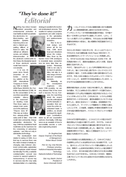
When QGIS starts, you are presented with the GUI as shown in the figure (the numbers 1 through 5 in yellow
circles are discussed below).
Figure 7.1: QGIS アラスカサンプルデータと GUI
ノート: ウィンドウの装飾（タイトルバーとか）は利用している オペレーティングシステムやウィンドウ
マネージャによって見かけが異なります.
QGIS の GUI は 5 つの領域に分割されています:
1. メニューバー
2. ツールバー
3. 地図凡例
4. 地図ビュー
5. ステータスバー
23
QGIS User Guide, リリース 2.2
これら 5 つの QGIS コンポーネントのインターフェースについては以下のセクションで詳しく説明されて
います. そのほかにキーボードショートカットとコンテキストヘルプの２つのセクションがあります.
7.1 メニューバー
メニューバーでは標準的な階層メニューを使って様々な QGIS の機能へのアクセスを提供しています. トッ
プレベルのメニューといくつかのメニューオプション, さらに各機能に対応した メニューバー上のアイコン
とキーボードショートカットについては以下に記述します. デフォルトのショートカットについてはこのセ
クションで解説します. しかしながらキーボードショートカットは Settings → Configure Shortcuts... で開
かれる Configure shortcuts ダイアログを使って手動で構成できます.
ほとんどのメニューオプションはツールに対応しているけど, 逆に対応していないこともあります, メニュー
はツールバーのようには構成されていません. ツールバーはそれぞれのチェックボックスエントリとしてあ
らわされているメニューオプションのリストツールを含んでいます. いくつかのメニューオプションは対応
するプラグインがロードされている時のみ表示されます. ツールとツールバーについてのさらに詳しい情報
は ツールバー 節を参照して下さい.
7.1.1 プロジェクト
メニューオプション
ショートカット
リファレンス
ツールバー
Ctrl+N
see プロジェクト
プロジェクト
Ctrl+O
see プロジェクト
see プロジェクト
see プロジェクト
プロジェクト
プロジェクト
保存
Ctrl+S
see プロジェクト
プロジェクト
名前をつけて保存...
Ctrl+Shift+S
see プロジェクト
プロジェクト
新規
開く
テンプレートを基に新規作成 →
最近利用したプロジェクト →
イメージで保存...
DXF エキスポート ...
新プリントコンポーザ
see 出力
see 出力
Ctrl+P
コンポーザマネージャ ...
プリントコンポーザ →
QGIS を終了する
24
see プリントコンポーザ
プロジェクト
see プリントコンポーザ
see プリントコンポーザ
プロジェクト
Ctrl+Q
Chapter 7. QGIS GUI
QGIS User Guide, リリース 2.2
7.1.2 編集
メニューオプション
ショートカット
リファレンス
ツールバー
取り消し
Ctrl+Z
see 高度なデジタイジング
先進的なデジタイズ
再実行
Ctrl+Shift+Z
see 高度なデジタイジング
先進的なデジタイズ
地物の切り取り
Ctrl+X
see 既存レイヤのデジタイズ
デジタジング
地物のコピー
Ctrl+C
see 既存レイヤのデジタイズ
デジタジング
Ctrl+V
see 既存レイヤのデジタイズ
属性テーブルの作業 参照
デジタジング
Ctrl+.
see 既存レイヤのデジタイズ
デジタジング
地物の移動
see 既存レイヤのデジタイズ
デジタジング
選択物の削除
see 既存レイヤのデジタイズ
デジタジング
地物の回転
see 高度なデジタイジング
先進的なデジタイズ
地物の簡素化
see 高度なデジタイジング
先進的なデジタイズ
リングの追加
see 高度なデジタイジング
先進的なデジタイズ
部分の追加
see 高度なデジタイジング
先進的なデジタイズ
リングの塗りつぶし
see 高度なデジタイジング
先進的なデジタイズ
リングの削除
see 高度なデジタイジング
先進的なデジタイズ
部分の削除
see 高度なデジタイジング
先進的なデジタイズ
地物の変形
see 高度なデジタイジング
先進的なデジタイズ
オフセットカーブ
see 高度なデジタイジング
先進的なデジタイズ
地物の分割
see 高度なデジタイジング
先進的なデジタイズ
部分の分割
see 高度なデジタイジング
先進的なデジタイズ
選択地物の結合
see 高度なデジタイジング
先進的なデジタイズ
選択された地物の属性を結合する
see 高度なデジタイジング
先進的なデジタイズ
ノードツール
see 既存レイヤのデジタイズ
デジタジング
ポイントシンボルを回転する
see 高度なデジタイジング
先進的なデジタイズ
地物のペースト
新規レイヤへの地物貼り付け →
地物の追加
編集モード切替
レイヤに対し
モードを有効にすると, レイヤタイプ (ポイント, ラインまたはポリゴン) に
よって異なる 編集 メニューの 地物の追加 アイコンが表示されます.
7.1.3 編集（おまけ）
メニューオプション
リファレンス
ツールバー
地物の追加
see 既存レイヤのデジタイズ
デジタジング
地物の追加
see 既存レイヤのデジタイズ
デジタジング
地物の追加
see 既存レイヤのデジタイズ
デジタジング
7.1. メニューバー
ショートカット
25
QGIS User Guide, リリース 2.2
7.1.4 ビュー
メニューオプション
ショートカット
リファレンス
ツールバー
地図のパン
地図ナビゲーション
選択部分に地図をパンする
地図ナビゲーション
拡大
Ctrl++
地図ナビゲーション
縮小
選択 →
Ctrl+-
地物情報表示
計測 →
Ctrl+Shift+I
全域表示
Ctrl+Shift+F
see 地物の選択と選択解除
地図ナビゲーション
属性
see 計測
属性
属性
地図ナビゲーション
レイヤの領域にズーム
選択部分のズーム
地図ナビゲーション
地図ナビゲーション
Ctrl+J
直前の表示領域にズーム
地図ナビゲーション
次表示領域にズーム
地図ナビゲーション
実際のサイズにズームする
地図整飾 →
地図ナビゲーション
整飾 参照
マップチップス
属性
新しいブックマーク
Ctrl+B
see 空間ブックマーク
属性
ブックマークを見る
Ctrl+Shift+B
see 空間ブックマーク
属性
再読み込み
Ctrl+R
地図ナビゲーション
7.1.5 レイヤ
メニューオプション
新規 →
埋め込みレイヤとグループ ...
ショートカット
リファレンス
新しいベクタレイヤの作成 を参照
see プロジェクトの入れ子
ツールバー
レイヤの管理
ベクタレイヤの追加
Ctrl+Shift+V
see ベクタデータの操作
レイヤの管理
ラスタレイヤの追加
Ctrl+Shift+R
see QGIS にラスタデータをロードする
レイヤの管理
PostGIS レイヤの追加
Ctrl+Shift+D
see PostGIS レイヤ
レイヤの管理
SpatiaLite レイヤの追加
Ctrl+Shift+L
see SpatiaLite レイヤ
レイヤの管理
MSSQL 空間レイヤの追加
Ctrl+Shift+M
see label_mssql
レイヤの管理
Oracle GeoRaster レイヤの追加
see Oracle Spatial GeoRaster プラグイン
レイヤの管理
SQL Anywhere レイヤの追加
see SQL Anywhere プラグイン
レイヤの管理
see WMS/WMTS クライアント
レイヤの管理
WCS レイヤの追加
WCS クライアント を参照
レイヤの管理
WFS レイヤの追加
see WFS および WFS-T クライアント
レイヤの管理
デリミテッドテキストレイヤの追加
see label_dltext
レイヤの管理
スタイルのコピー
see スタイルメニュー
スタイルの貼り付け
see スタイルメニュー
WMS/WMTS レイヤの追加
Ctrl+Shift+W
次のページに続く
26
Chapter 7. QGIS GUI
QGIS User Guide, リリース 2.2
Table 7.1 – 前のページからの続き
ショートカット
リファレンス
メニューオプション
ツールバー
属性テーブルのオープン
属性テーブルの作業 参照
属性
編集モード切替
see 既存レイヤのデジタイズ
デジタジング
レイヤの編集を保存する
see 既存レイヤのデジタイズ
デジタジング
see 既存レイヤのデジタイズ
デジタジング
カレントエディット →
名前をつけて保存...
選択をベクタファイルとして保存...
属性テーブルの作業 参照
レイヤの削除
Ctrl+D
レイヤの複製
レイヤの CRS を設定する
レイヤの CRS をプロジェクトに設定する
プロパティ
クエリ...
Ctrl+Shift+C
ラベリング
全体図に追加
Ctrl+Shift+O
レイヤの管理
全てのレイヤを表示
Ctrl+Shift+U
レイヤの管理
全てのレイヤを隠す
Ctrl+Shift+H
レイヤの管理
全体図に全て追加
全体図から全て削除
7.1.6 設定
メニューオプション
パネル →
ツールバー →
フルスクリーンモードへ切り替え
プロジェクトプロパティ ...
ショートカット
リファレンス
see パネルとツールバー
see パネルとツールバー
ツールバー
F 11
Ctrl+Shift+P
カスタム CRS ...
スタイルマネージャ...
ショートカットの構成 ...
カスタマイゼーション ...
オプション ...
スナッピングオプション ...
see プロジェクト
see カスタム空間参照システム
see vector_style_manager
see カスタマイゼーション
オプション 参照
7.1.7 プラグイン
メニューオプション
プラグインの管理とインストール
Python コンソール
ショートカット
リファレンス
ツールバー
see The Plugins Menus
QGIS を最初に立ち上げた時はすべてのコアプラグインがロードされるわけではありません.
7.1. メニューバー
27
QGIS User Guide, リリース 2.2
7.1.8 ベクタ
メニューオプション
オープンストリートマップ →
ショートカット
リファレンス
see OpenStreetMap ベクタの読み込み
解析ツール →
see fTools プラグイン
調査ツール →
see fTools プラグイン
ジオプロセッシングツール →
see fTools プラグイン
ジオメトリツール →
see fTools プラグイン
データマネジメントツール →
see fTools プラグイン
ツールバー
QGIS を最初に立ち上げた時はすべてのコアプラグインがロードされるわけではありません.
7.1.9 ラスタ
メニューオプション
ラスタ計算機 ...
ショートカット
リファレンス
see ラスタ計算機
ツールバー
QGIS を最初に立ち上げた時はすべてのコアプラグインがロードされるわけではありません.
7.1.10 プロセシング
メニューオプション
ショートカット
リファレンス
ツールボックス
see ツールボックス
グラフィカルモデラー
グラフィカルモデラー 参照
履歴とログ
ツールバー
see 履歴マネージャ
オプションと構成
プロセッシングフレームワークを構成する 参照
結果ビューア
see 外部アプリケーションの設定
コマンダー
Ctrl+Alt+M
The SEXTANTE Commander 参照
QGIS を最初に立ち上げた時はすべてのコアプラグインがロードされるわけではありません.
7.1.11 ヘルプ
メニューオプション
ヘルプコンテンツ
What’s This?
API 文書
コマーシャルサポートが必要ですか?
QGIS ホームページ
ショートカット
リファレンス
ツールバー
F1
ヘルプ
Shift+F1
ヘルプ
Ctrl+H
QGIS のバージョンをチェックする
アバウト
QGIS スポンサー
上記にリストされている Linux
メニューバーは KDE ウィンドウマネージャのデフォルトのひとつであ
ることに注意してください.GNOME では 設定 メニューは異なる内容でそのアイテムはここにあります:
28
Chapter 7. QGIS GUI
QGIS User Guide, リリース 2.2
プロジェクトプロパティ
オプション
ショートカットの構成
スタイルマネージャ
プロジェクト
編集
編集
編集
カスタム CRS
パネル →
ツールバー →
フルスクリーンモードへ切り替え
タイルスケールスライダー
ライブ GPS トラッキング
編集
ビュー
ビュー
ビュー
ビュー
ビュー
7.2 ツールバー
ツールバーではメニューのほとんどと同じ機能を提供している上に対話的に地図を操作する機能を提供し
ています. ツールバーのそれぞれのアイテムではポップアップヘルプが提供されています. マウスでアイテ
ムの上を動かすとツールの簡単な説明が表示されます.
それぞれのメニューバーは必要に応じて移動できます. さらに. それぞれのメニューバーはツールバー上に
マウスポインタを置き、右ボタンでコンテキストメニューを使ってオフにすることができます ( パネルと
ツールバー も参照して下さい).
ちなみに: ツールバーの復元
もしあなたの環境でツールバーが隠れてしまった場合メニューの Settings → Toolbars → を選択すると復帰
させることができます. ツールバーがウィンドウの下に隠れ, その現象が QGIS で時々発生する場合はレ
ジストリ \HKEY_CURRENT_USER\Software\QGIS\qgis\UI\state を削除して下さい. QGIS を再
起動すると, そのキーはデフォルト値で上書きされます, デフォルト値ではツールバーは再び表示されるよ
うになります.
7.3 地図凡例
The map legend area lists all the layers in the project. The checkbox in each legend entry can be used to show or
hide the layer.
レイヤは選択してドラッグで上下に移動することによって Z オーダリングを変えることができます.Z オー
ダリングとは, 凡例のリストでの表示順が地図表示のレイヤ表示順になることです.
ノート: この動作は ‘レイヤ順序’ パネルによって上書きできます.
凡例ウィンドウ内のレイヤはグループを構成することができます. その方法は２つあります：
1. Right click in the legend window and choose Add New Group. Type in a name for the group and press
Enter. Now click on an existing layer and drag it onto the group.
2. 凡例ウィンドウでいくつかのレイヤを選択してマウス右ボタンをクリックして Group Selected を選択
して下さい. 選択されたレイヤで自動的に新しいグループが作られます.
あるレイヤをグループからはずしたい場合はレイヤ名をドラッグしてグループ外に持っていくかマウス右
ボタンクリックして Make to toplevel item を選択して下さい. グループは他のグループからネストすること
ができます.
グループ用チェックボックスを使うとクループ内全レイヤの表示, 非表示を 1 回のクリックで行えます.
マウス右ボタンで表示されるコンテキストメニューの内容は凡例で選択されているレイヤがラスタなのか
Toggle editing
ベクタなのかによって異なります. GRASS ベクタレイヤの場合
は利用できません. GRASS
ベクタレイヤの編集についての情報は GRASS ベクタレイヤのデジタイジングと編集 を参照して下さい.
7.2. ツールバー
29
QGIS User Guide, リリース 2.2
ラスタレイヤ選択時のマウス右ボタンメニュー
• レイヤの領域にズーム
• 最適スケールにズームする (100%)
• 現在の領域を使って引き伸ばす
• 全体図に表示
• 削除
• 複製
• レイヤ CRS を設定する
• レイヤの CRS をプロジェクトに設定する
• 名前をつけて保存 ...
• プロパティ
• 改名
• スタイルコピー
• Add New Group
• Expand all
• Collapse all
• Update Drawing Order
さらに、レイヤの位置と選択に従って
• アイテムをトップレベルに移動する
• 選択されたレイヤをグループにする
ベクタレイヤ選択時のマウス右ボタンメニュー
• レイヤの領域にズーム
• 全体図に表示
• 削除
• 複製
• レイヤ CRS を設定する
• レイヤの CRS をプロジェクトに設定する
• 属性テーブルのオープン
• 編集モード切替 ( GRASS レイヤでは利用できません)
• 名前をつけて保存 ...
• Save Selection As
• フィルター
• 地物数表示
• プロパティ
• 改名
• スタイルコピー
• Add New Group
• Expand all
• Collapse all
30
Chapter 7. QGIS GUI
QGIS User Guide, リリース 2.2
• Update Drawing Order
さらに、レイヤの位置と選択に従って
• アイテムをトップレベルに移動する
• 選択されたレイヤをグループにする
レイヤグループ用マウス右ボタンメニュー
• グループにズームする
• 削除
• グループ CRS の設定
• 改名
• Add New Group
• Expand all
• Collapse all
• Update Drawing Order
It is possible to select more than one layer or group at the same time by holding down the Ctrl key while selecting
the layers with the left mouse button. You can then move all selected layers to a new group at the same time.
You may also delete more than one layer or group at once by selecting several layers with the Ctrl key and
pressing Ctrl+D afterwards. This way, all selected layers or groups will be removed from the layers list.
7.3.1 レイヤの標示順序から独立した凡例の操作
凡例の順序とは独立に描画順序を指定できるウィジェットがあります. この機能はメニュー Settings → Panels
→ Layer order で有効にすることができます. 地図上でのレイヤ描画順序をここで指定することができます.
この指定でたとえば重要さの順にレイヤを描画することができます, しかしこのままでは依然として修正
した結果の順にレイヤが表示されます ( figure_layer_order を参照して下さい). レイヤリストの下にある
Control rendering order をチェックするとデフォルトの動作と異なる動作をするでしょう.
7.4 地図ビュー
これは QGIS の “ビジネスエンド” です - 地図はこの領域に表示されます! 地図はこのウィンドウに表示さ
れあなたが選択してロードしたベクタとラスタレイヤに依存しています (以下のセクションにどのようにレ
イヤをロードするかの詳しい情報があります). マップビューでは地図のパンや (地図の表示領域を別の場所
に移動すること) ズームインとズームアウトができます. 地図ではその他にも上記のツールバーの解説で述
べられているような多彩な操作ができます. マップビューと凡例はお互い密接に関係しています - 凡例の領
域で変更を行うと地図の表示に変更が加わります.
ちなみに: マウスホィールを使って地図をズームします
マウスホィールを使って地図のズームインとズームアウトを行うことができます. マウスカーソルを地図
エリアの中に置きホィールを前方 (あなたの側から) ロールするとズームインを行えます, そして手前に (あ
なたの側に) ロールするとズームアウトします. マウスカーソルの位置がズームの中心になります. マウス
ホィールのズーム動作については Settings → Options メニューの Map tools タブでカスタマイズができます.
ちなみに: 矢印キーとスペースバーを使った地図パンニング
矢印キーを使ってパンを行うことができます. マウスカーソルを地図エリアにおきクリックした後右矢印
キーを押すと東にパンします, 左矢印キーを押すと西にパンします, 上矢印キーを押すと北にパンします. 下
矢印キーを押すと南にパンします. またスペースバーかマウスホィールを使ってパンを行うことができます.
この場合スペースバーを押しながらマウスを動かすかマウスホィールをクリックして下さい.
7.4. 地図ビュー
31
QGIS User Guide, リリース 2.2
Figure 7.2: レイヤの順序から独立した凡例の定義
7.5 ステータスバー
ステータスバーにはマウスポインターがマップビュー内を移動した時の位置の地図座標 (たとえばメート
ルか度数) が表示されます. 座標表示の左側は小さいボタンになって いてマウスの位置座標の表示かマップ
ビューの拡大、縮小した場合の現在の四隅の座標 表示を行うかの切り替えを行います.
座標ディスプレイの隣に縮尺ディスプレイがあります. ここにはマップビューの縮尺が表示されます. ズー
ムインまたはズームアウトを行うと QGIS はカレントスケールを表示します. また事前定義された 1:500 か
ら 1:1000000 の間のスケールセレクタがそこに実装されています.
ステータスバーの中にあるプログレスバーには各レイヤをマップビューに描画する処理の進行状況が表示
されます. ラスタレイヤで統計処理をするような場合プログレスバーは非常に長い処理の進行状態を 表示
することになります.
もし新しいプラグインのリリースやプラグインのアップデートが行われた場合ステータスバーの左端にメッ
セージが表示されます. ステータスバーの右側にはマップビューでのレイヤレンダリングを一時的にとめる
小さなチェックボックスがあります (以下の レンダリング セクションを参照して下さい).
急に現在の地図レンダリングプロセスを停止します.
アイコンは緊
レンダ機能の右側に現在のプロジェクト CRS の EPSG コードとプロジェクションアイコンが表示されてい
ます. これをクリックすると現在のプロジェクトの投影プロパティを開くことができます.
ちなみに: マップキャンバスにおける正しい縮尺を計算する
When you start QGIS, the default units are degrees, and this means that QGIS will interpret any coordinate in your
layer as specified in degrees. To get correct scale values, you can either change this setting to meters manually in
CRS status
the General tab under Settings → Project Properties, or you can select a project CRS clicking on the
icon in the lower right-hand corner of the status bar. In the last case, the units are set to what the project projection
specifies (e.g., ‘+units=m’).
.
32
Chapter 7. QGIS GUI
Chapter 8
一般ツール
8.1 キーボードショートカット
QGIS は多くの機能のデフォルトキーボードショートカットを提供しています. セクション メニューバー に
それらは記述されています. さらにメニューオプション Settings → Configure Shortcuts を使うとデフォルト
キーボードショートカットを変更して新しいキーボードショートカットを QGIS の機能に加えることがで
きます.
Figure 8.1: ショートカットオプションの定義
(Gnome)
構成はとても簡単です. リストから機能を選択し [変更], [無し] を設定 または [デフォルトを設定] をクリッ
クして下さい. あなた自身の構成を作成したら, その設定を XML ファイルで保存して他の QGIS インスト
レーションでロードして利用することができます.
8.2 コンテキストヘルプ
特定のトピックでヘルプが必要な場合多くのダイアログに実装されている [Help] ボタンでコンテキストヘ
ルプを利用することができます- サードパーティプラグインでは専用のウェッブページを指し示すことを注
意して下さい.
33
QGIS User Guide, リリース 2.2
8.3 レンダリング
デフォルトで QGIS レンダラはマップキャンパスに含まれる全ての可視レイヤ表示を更新します. このイベ
ントはマップキャンバスに含まれるものすべてをリフレッシュします:
• レイヤの追加
• パンまたはズーム
• QGIS ウィンドウのリサイズします
• レイヤまたはレイヤ群の表示、非表示を変更します
QGIS ではいくつもの方法で描画プロセスを管理できます.
8.3.1 スケール依存レンダリング
スケール依存レンダリングを利用するとあるレイヤが表示される最小と最大のスケールを指定することが
できます. スケール依存レンダリングを設定する場合レイヤを凡例でダブルクリックして プロパティ ダイ
アログを開いて下さい. 一般情報 タブで,
最小と最大の縮尺値を設定して下さい. .
縮尺に応じた表示設定 チェックボックスをアクティブにして
QGIS ステータスバーでスケール値を見ることで, そのレイヤを表示するのと表示しないスケール値を決め
ることができます.
8.3.2 地図レンダリングの制御
地図レンダリングは以下に記述される様々な方法で制御することができます:
描画の中断
描画を中止したい場合はステータスバーの右側角にある
Render チェックボックスをクリックしてくだ
さい.
Render がチェックされていない場合 QGIS はセクション レンダリング に記述されているあらゆ
るイベントに反応せずキャンバスに再描画を行いません. 地図描画を行わないほうがいい場合は以下のよう
な場合があります:
• 沢山のレイヤを追加して描画する前に描画方法を編集したい場合
• データ量が多いレイヤを追加して描画する前に縮尺依存描画条件を指定したい場合
• データ量が多いレイヤを追加して描画する前に特定の位置にズームしておきたい場合
• 上記の場合のいくつかの組み合わせ
Checking the
Render checkbox enables rendering and causes an immediate refresh of the map canvas.
レイヤ追加オプションの設定
新しくレイヤを追加した時に, すぐに描画しないオプションを設定できます. これはレイヤが地図に追加さ
れた時に, 地図凡例の可視属性チェックボックスがデフォルトでチェックされないことを意味します. このオ
プションを指定するためには 設定 → オプション → を選択して レンダリング タブをクリックしてくださ
By default new layers added to the map should be displayed のチェックを解除してください. すると, 地
い.
図に追加されたレイヤの表示属性は不可視の状態がデフォルトになります.
34
Chapter 8. 一般ツール
QGIS User Guide, リリース 2.2
描画の中断
地図描画を中断したい場合は ESC キーを押して下さい. これにより地図キャンパスの更新が中断され地図
の一部が描画された状態になります. ESC キーを押してから地図描画が中断されるまで少し時間がかかり
ます.
ノート: 現在描画中断機能は利用できません - これは Qt4 のポートに依存しています, なぜならばユーザー
インターフェース (UI) に問題が発生してクラッシュするからです.
描画中に地図表示を更新する
地図に地物が描画更新されるオプションの設定を行うことができます. デフォルトで, QGIS はレイヤの描
画が終了するまで地物を表示しません. 地物がデータストアから読まれるときに表示を更新したい場合, メ
ニューオプションの Settings → Options を選択して Rendering メニューをクリックして下さい. 描画更新を
行う適切な地物の数を設定して下さい. 設定値が 0 の場合描画時の更新を行いません (これがデフォルトで
す). 設定値が小さい場合地物読み込み時に地図キャンバスの継続的な更新が行われパフォーマンスが低下
します. 推奨値は 500 以上です.
描画品質への影響
描画品質に影響がある 2 個のオプションがあります. メニュー 設定 → オプション を選択して レンダリ
ング タブをクリックして以下のチェックボックスを選択、または非選択して下さい.
•
線のジャギーを目立たなくします (描画パフォーマンスが低下します)
•
ポリゴンの不正な塗りつぶしを修正します
スピードアップレンダリング
描画品質に影響がある 2 個のオプションがあります. メニュー 設定 → オプション を選択して QGIS オプ
ションダイアログを開き レンダリング タブをクリックして以下のチェックボックスを選択、または非選択
して下さい.
•
•
バックバッファを有効にする. このオプションはキャンセル機能を無効にすることでグラフィック
のパフォーマンスを向上させています, そして地物を追加しながら描画します . これがチェックされ
ていない場合 Number of features to draw before updating the display を設定できます, そうでない場
合このオプションは非アクティブです.
再描画の速度を上げられる場合にレンダのキャッシュを利用します
8.4 計測
計測は投影座標系 (e.g., UTM) と投影されていないデータ内で機能します. ロードされたマップは地理座標
系（緯度/経度）で定義され、ラインや面積の計測結果は正確ではないでしょう. 必要に応じ、適切なマップ
の座標系（ 投影法の利用方法 のセクションを参照）を設定することで解決します。すべての計測モジュー
ルはデジタイジングモジュール由来のスナップ設定が使用されています. ベクターレイヤのラインやエリア
にそって計測をしたい場合、これは便利です.
計測ツールを選択するためには
8.4. 計測
をクリックして使いたいツールを選択してください.
35
QGIS User Guide, リリース 2.2
8.4.1 距離, 面積と角度の計測
Measure Line
: QGIS では与えられた点の間の実距離を定義された楕円体にしたがって測ることができます.
この機能を構成するためにはメニューオプション Settings → Options を選択して, Map tools タブをクリック
して最適な楕円体を選択して下さい. そこではラバーバンドの色と最適な計測単位 (メーターまたはフィー
ト) と角度の単位 (度, ラディアン と gon) も指定できます. このツールを使うと地図上にポイントをクリッ
クできます. それぞれのセグメントの長さと合計値が計測ウィンドウに表示されます. 計測を終了したい場
合はマウス右ボタンをクリックして下さい.
Figure 8.2: 距離の計測
(Gnome)
面積の計測
: 面積も計測することができます。計測ウィンドウで、累積の面積サイズが表示されます。さ
らに、計測ツールでは現在選択しているレイヤにスナップする場合のスナップ許容値を設定できます ( ス
ナップ許容量と検索半径の設定 のセクションを参照)。ラインフィーチャまたはポリゴンの周辺に正確に
沿って計測したい場合は、そのスナップ許容値を設定し、レイヤを選択します。計測ツールを使う賽、マ
ウスをクリックするたびに（許容値の設定内で）レイヤをスナップします。
Figure 8.3: 面積の計測
(Gnome)
Measure Angle
: 角度を計測することができます. カーソルが十字の形状になります. 測定したい最初のセグ
メントをクリックし, 計測を希望する角度を描くようにカーソルを移動します. 計測結果がポップアップダ
イアログに表示されます.
Figure 8.4: 角度の計測
(Gnome)
8.4.2 地物の選択と選択解除
QGIS ツールバーはマップキャンバスで地物を選択するためにいくつかのツールを提供しています. １つま
たはいくつかの地物をクリックのみで選択する場合は
•
36
をクリックし, あなたのツールを選択して下さい.
1 個の地物を選択する
Chapter 8. 一般ツール
QGIS User Guide, リリース 2.2
•
矩形による地物選択
•
多角形による地物選択
•
フリーハンドによる地物選択
•
半径による地物選択
選択されている地物をすべて解放したい場合は
すべてのレイヤから地物選択を取り消す
をクリックして下さい.
8.5 地物情報表示
地物特定をするとマップキャンバスと対話的に操作してポップアップウィンドウで属性データを表示でき
ます. 地物を特定する場合 View → Identify features を選択するか Ctrl + Shift + I をキーボードで押
すかツールバーの,
Identify features
アイコンをクリックして下さい.
もしあなたが複数の地物をクリックした場合 I, Identify results ダイアログは全地物の属性をリストします.
最初のアイテムは結果のアイテムの数でレイヤ名が続きます. 最初の子アイテムはフィールド名と値です.
最後に地物の全情報が表示されます.
このウィンドウはカスタムフィールドを表示するためにカスタマイズできますがデフォルトで 3 種類の情
報を表示します:
• アクション: 地物情報表示ウィンドウにアクションの追加ができます. アクションラベルをクリック
するとアクションを実行できます デフォルトで編集用フォーム表示アクションのみが登録されてい
ます.
• 由来：この情報は、他の情報から計算するか導き出されたものです。クリックされた位置のマップ単
位での座標値、x,y 座標、マップ単位でのポリゴンの境界の長さ、地物 ID を見つけることができます。
• データ属性：これは、データの属性フィールドのリストです。
Figure 8.5: 地物情報表示ダイアログ
(Gnome)
ウィンドウの下部には 5 個のアイコンがあります:
•
ツリーを展開する
•
ツリーを折りたたむ
•
デフォルトの動作
8.5. 地物情報表示
37
QGIS User Guide, リリース 2.2
•
属性をコピーする
•
選択した HTML のレスポンスを表示する
その他の機能は、識別されたアイテムのコンテキストメニューにあります。たとえば、コンテキストメニュー
から次のことができます：
• 地物フォームの表示
• 地物のズーム
• 地物のコピー: すべての地物, のジオメトリと属性をコピーします;
• 属性値のコピー: あなたがクリックした属性値のみをコピーします。
• 地物の属性をコピーする:属性のみをコピーする;
• 結果のクリア:ウィンドウ内の結果が削除されます
• ハイライトのクリア:地図上でハイライトしている地物が除去されます
• すべてをハイライトする
• レイヤをハイライトする
• レイヤのアクティベート: アクティベートするレイヤの選択
• レイヤプロパティ: レイヤプロパティウィンドウを表示する
• すべてを展開する
• すべてを折りたたむ
8.6 整飾
QGIS の整飾にはグリッド, 著作権ラベル、北向き矢印とスケールバーが含まれています. これらは地図描画
のエレメントとして地図を ’整飾 ’するために用いられます。
8.6.1 グリッド
グリッド
では座標のグリッドと座標注記をマップキャンバスに追加します。
Figure 8.6: グリッドダイアログ
38
Chapter 8. 一般ツール
QGIS User Guide, リリース 2.2
1. Select from menu View → Decorations → Grid. The dialog starts (see figure_decorations_1).
2. マップキャンバスにロードされているレイヤにしたがって
してグリッドの設定を行って下さい.
Enable grid チェックボックスを有効に
3. マップキャンバスにロードされているレイヤにしたがって
有効にしてアノテーションの定義を行ってください.
Draw annotations チェックボックスを
4. Click [Apply] to verify that it looks as expected.
5. [OK] をクリックしてダイアログを閉じます.
8.6.2 著作権ラベル
Copyright label
は好みのテキストを使用して, マップに著作権ラベルを追加します.
Figure 8.7: 著作権ダイアログ
1. メニューの ビュー → 地図整飾 → 著作権ラベル を選択します。ダイアログが表示されます ( figure_decorations_2 を参照すること)。
2. マップ上に配置したいテキストを入力してください. 例に示す通り HTML を使用することができます.
3. Choose the placement of the label from the Placement
4. Make sure the
combo box.
Enable Copyright Label checkbox is checked.
5. [OK] をクリックして下さい.
上記の例のように QGIS はデフォルトで著作権シンボルを日付つきで地図キャンバスの右下に表示します.
8.6.3 北向き矢印
北向き矢印
を使うとシンプルな北向き矢印をマップキャンバスに置くことができます. 現在 1 種類のスタ
イルのみが利用できます. 矢印の角度は調整可能ですし, また QGIS が自動的に方向を設定することもでき
ます. もし QGIS が方位を決める方法を選択すると最良の矢印の方向を指し示します. 矢印を置く場所は 4
つのオプションがあります, マップキャンバスの 4 つの隅です.
8.6.4 スケールバー
スケールバー
はシンプルなスケールバーをマップキャンバスに追加します. スタイルと位置, バーの上の
ラベルを設定できます.
8.6. 整飾
39
QGIS User Guide, リリース 2.2
Figure 8.8: 北向き矢印ダイアログ
Figure 8.9: スケールバーダイアログ
QGIS はあなたのマップフレームと同じ単位スケールを表示することをサポートしています. もしレイヤの
単位がメートルであるなら, フィート単位のスケールバーを作成することはできません. 同様に, 度数単位を
使用している場合はメートル単位で距離を表示するスケールバーを作成することはできません.
スケールバーを追加するために：
1. メニューの ビュー → 地図整飾 → 著作権ラベル を選択して下さい. ダイアログが表示されます (
figure_decorations_4 を参照して下さい).
2. Choose the placement from the Placement
3. Scale bar style
combo box.
コンボボックスからスタイルを選択して下さい.
でバーの色を選択するか, デフォルト
4. Color of bar
の黒を使用して下さい.
5. バーの大きさとラベルの設定 Size of bar
.
6. Make sure the
Enable scale bar checkbox is checked.
7. オプションで
Automatically snap to round number on resize もチェックできます.
8. [OK] をクリックして下さい.
ちなみに: 整飾の設定
.qgs プロジェクトを保存する際, グリッド, 方位記号, スケールバーと著作権ラベルに加えた変更はそのプ
ロジェクトに保存され, 次回プロジェクトをロードした際に復元されます.
40
Chapter 8. 一般ツール
QGIS User Guide, リリース 2.2
8.7 アノテーションツール
Text Annotation
属性ツールバーの
ツールを使うと QGIS マップキャンバスに書式整形されたテキストを表
示したバルーンを表示できます. Text Annotation ツールを使ってマップキャンバスをクリックして下さい.
Figure 8.10: アノテーションテキストダイアログ
項目をダブルクリックすると、さまざまなオプションを含むダイアログが開きます。フォーマットされた
テキストやその他の項目の設定値を入力するテキストエディタがあります。例えば、マップの位置（マー
カーシンボルが表示された）に関する項目またはスクリーンの位置（マップに関連していない）における
選択肢を持ちます。この項目はマップの位置（マップマーカーをドラッグすることにより）が移動し、ま
たはバルーンのみが移動します。アイコンは、GIS の主題図の一部であり、それらも、他の主題図におい
てデフォルトとして用いられます。
The
Move Annotation
tool allows you to move the annotation on the map canvas.
8.7.1 HTML 注記
Html Annotation
属性ツールバーの
ツールを使うと QGIS マップキャンバスに html ファイルを内容とした
バルーンを表示することができます. Html Annotation ツールを使ってマップキャンバスをクリックして下
さい, そして html ファイルのパスを追加して下さい.
8.7.2 SVG 注記
SVG Annotation
属性ツールバーにある
ツールを使うと QGIS マップキャンバスに SVG シンボルを描画し
たバルーンを表示することができます. SVG Annotation ツールを使いマップキャンバスをクリックした後に
ダイアログで SVG ファイルのパスを追加して下さい.
8.7.3 注記の書式設定
Form Annotation
加えてあなたは自分独自のアノテーションフォームを作ることができます.
ツールはベ
クタレイヤの属性を Qt デザインフォームでカスタマイズして表示するためには便利なツールです ( figure_custom_annotation 参照). これは Identify features ツールのデザイナーに似ていますが注記アイテムを
8.7. アノテーションツール
41
QGIS User Guide, リリース 2.2
表示します. Tim Sutton のビデオ https://www.youtube.com/watch?v=0pDBuSbQ02o に詳しい情報があるので
見てください.
Figure 8.11: カスタマイズされた qt デザイナアノテーションフォーム
ノート: If you press Ctrl+T while an Annotation tool is active (move annotation, text annotation, form annotation), the visibility states of the items are inverted.
8.8 空間ブックマーク
空間ブックマークを使用すると地理的な場所を” ブックマーク” し、あとでその位置に戻ることができます。
8.8.1 ブックマークの作成
ブックマークを作るには：
1. 関心のある領域にズームまたはパンします。
2. メニューオプション View → New Bookmark を選択するか Ctrl-B を押して下さい.
3. ブックマークを説明する名称（255 文字まで）を入力します。
4. ブックマークを追加するためには Enter を入力するかブックマークを削除するためには [Delete] を
押して下さい.
同じ名称で複数のブックマークを所有できることにご注意ください。
8.8.2 ブックマークの操作
ブックマークを利用または管理する場合メニューオプション View → Show Bookmarks を選択して下さい.
Geospatial Bookmarks ダイアログを使うとブックマークへのズームと削除ができます. ブックマーク名や座
標は編集できません.
42
Chapter 8. 一般ツール
QGIS User Guide, リリース 2.2
8.8.3 ブックマークへのズーム
From the Geospatial Bookmarks dialog, select the desired bookmark by clicking on it, then click [Zoom To]. You
can also zoom to a bookmark by double-clicking on it.
8.8.4 ブックマークの削除
ブックマークを削除するには 地理空間ブックマーク ダイアログでブックマークを選択し、[削除] をクリッ
クして下さい. 削除を確定する場合は [はい] をクリックし, 削除をキャンセルする場合には [いいえ] をク
リックして下さい.
8.9 プロジェクトの入れ子
あなたのプロジェクトに他のプロジェクトファイルからコンテンツを埋め込む場合 Layer → 埋め込みレイ
ヤとグループ を選択して下さい.
8.9.1 埋め込みレイヤ
次のダイアログで, 他のプロジェクトのレイヤを埋め込むことができます.
1. Press
to look for another project from the Alaska dataset.
2. プロジェクトファイルの grassland を選択して下さい. あなたはプロジェクトの中身を表示するこ
とができます ( figure_embed_dialog を参照してください).
3. Press Ctrl and click on the layers grassland and regions. Press [OK]. The selected layers are
embedded in the map legend and the map view now.
Figure 8.12: 埋め込むためのレイヤとグループを選択する
埋め込まれているレイヤが編集可能になっている間, スタイルやラベリングのようなプロパティは変更する
ことができません.
8.9.2 埋め込みレイヤの除去
組み込みレイヤを右ボタンクリックして
Remove
を選択して下さい.
.
8.9. プロジェクトの入れ子
43
Chapter 9
QGIS 設定
QGIS は 設定 メニューを使って高度な設定をすることができます. パネル, ツールバー, プロジェクトプロ
パティ, オプションとカスタマイゼーションを選択してみてください.
9.1 パネルとツールバー
In the Panels→ menu, you can switch on and off QGIS widgets. The Toolbars→ menu provides the possibility to
switch on and off icon groups in the QGIS toolbar (see figure_panels_toolbars).
Figure 9.1: パネルとツールバーメニュー
ちなみに: QGIS オーバービューを有効にする
QGIS では追加されたレイヤの全範囲のビューを提供するオーバービューパネルを提供します. これは 設
ビュー → パネル メニューの下から選択することができます. ビュー内で現在のマッ
定 → パネル または
45
QGIS User Guide, リリース 2.2
プ範囲を示す長方形があります. これによって現在見ているマップのどのエリアかを決定することができ
ます. マップオーバービューのレイヤにラベリングが設定されていても、ラベルはマップのオーバービュー
にレンダリングされないことに注意してください. オーバービューで現在の領域を示す赤い四角形をクリッ
ク・ドラッグすると、メインマップのビューもそれに応じて更新されます.
ちなみに: ログメッセージの表示
Log Messages in the menu
Settings → Panels
It’s possible to track the QGIS messages. You can activate
or View → Panels and follow the messages that appear in the different tabs during loading and operation.
9.2 プロジェクトのプロパティ
In the properties window for the project under
Settings → Project Properties or
ties, you can set project-specific options. These include:
Project → Project Proper-
• In the General menu, the project title, selection and background color, layer units, precision, and the option
to save relative paths to layers can be defined. If the CRS transformation is on, you can choose an ellipsoid
for distance calculations. You can define the canvas units (only used when CRS transformation is disabled)
and the precision of decimal places to use. You can also define a project scale list, which overrides the
global predefined scales.
• The CRS menu enables you to choose the Coordinate Reference System for this project, and to enable
on-the-fly re-projection of raster and vector layers when displaying layers from a different CRS.
• 3 番目の 情報検索レイヤ メニューからどのレイヤを情報探索ツールで確認できるようにするか (ある
いはしないか) を設定できます (複数レイヤを確認する方法は オプション セクションの “マップツー
ル” の項目を見てください).
• The Default Styles menu lets you control how new layers will be drawn when they do not have an existing
.qml style defined. You can also set the default transparency level for new layers and whether symbols
should have random colours assigned to them.
• OWS Server タブは QGIS サーバの WMS と WFScapabilities、エクステントと CRS の制限についての
情報を定義します。
• マクロ メニューは Python マクロの編集のために使います. 現時点では: openProject(),
saveProject() そして closeProject() の 3 つのマクロのみ使用可能です.
• The Relations menu is used to define 1:n relations. The relations are defined in the project properties dialog.
Once relations exist for a layer, a new user interface element in the form view (e.g. when identifying a
feature and opening its form) will list the related entities. This provides a powerful way to express e.g. the
inspection history on a length of pipeline or road segment. You can find out more about 1:n relations support
in Section １対多リレーションの作成.
9.3 オプション
Some basic options for QGIS can be selected using the Options dialog. Select the menu option Settings →
Options. The tabs where you can customize your options are described below.
9.3.1 一般情報メニュー
アプリケーション
• スタイル (QGIS 再起動が必要です)
‘Cleanlux’ ( ) の中から選択します。
46
を選択し ‘Oxygen’,’Windows’,’Motif’,’CDE’, ‘Plastique’ と
Chapter 9. QGIS 設定
QGIS User Guide, リリース 2.2
Figure 9.2: QGIS でのマクロ設定
• アイコンテーマ
• Define the Icon size
を定義します。現時点では’ デフォルト’ のみ利用可能です。
.
• フォント を定義します。
QT 規定値 とユーザ定義のフォントから選択します。
• メッセージやダイアログのタイムアウト設定
•
起動時のスプラッシュスクリーンを隠す
•
起動時にチップスを表示する
•
グループボックスのタイトルを太字にする
•
QGIS スタイルのグループボックス
•
色選択ダイアログの随時更新
を変更します。
プロジェクトファイル
• 起動時にプロジェクトを開く |selectstring|（’ 新規’、’ 最新’ と ‘指定’ の間から選択します。） ‘指定’
を選択した時プロジェクトを定義するために |browsebutton| を使用します。
•
既定のプロジェクトから新プロジェクトを作成する. 現在のプロジェクトを既定プロジェクトとし
て指定する または 既定を解除 ボタンをクリックすることができます. またユーザが作成したプロジェ
クトテンプレートをファイルやディレクトリを指定するとブラウズすることができます. プロジェク
ト → テンプレートをもとに新規作成 というエントリでそれができます. プロジェクトテンプレート
既定のプロジェクトから新プロジェクトを作成する をアクティブにし
を保存したい場合は最初に
てプロジェクトテンプレートフォルダーにプロジェクトを保存してください.
•
必要に応じプロジェクトとデータソースの変更の保存を促す
•
QGIS の旧バージョンで保存したプロジェクトファイルを開く際に警告する
• Enable macros
. This option was created to handle macros that are written to perform an action on
project events. You can choose between ‘Never’, ‘Ask’, ‘For this session only’ and ‘Always (not recommended)’.
9.3. オプション
47
QGIS User Guide, リリース 2.2
9.3.2 システムメニュー
環境
System environment variables can now be viewed, and many configured, in the Environment group (see figure_environment_variables). This is useful for platforms, such as Mac, where a GUI application does not necessarily inherit the user’s shell environment. It’s also useful for setting and viewing environment variables for
the external tool sets controlled by the Processing toolbox (e.g., SAGA, GRASS), and for turning on debugging
output for specific sections of the source code.
•
Use custom variables (restart required - include separators). You can [Add] and [Remove] variables.
Already-defined environment variables are displayed in Current environment variables, and it’s possible to
filter them by activating
Show only QGIS-specific variables.
Figure 9.3: QGIS におけるシステム環境の多様性
プラグインパス
[Add] or [Remove] Path(s) to search for additional C++ plugin libraries
9.3.3 データソースメニュー
地物属性とテーブル
•
48
ドックウィンドウで属性テーブルを開く（QGIS の再起動が必要）‘
Chapter 9. QGIS 設定
QGIS User Guide, リリース 2.2
•
Copy selected rows to clipboard
Copy geometry in WKT representation from attribute table. When using
from the Attribute table dialog, this has the result that the coordinates of points or vertices are also copied
to the clipboard.
• 属性テーブルの動作
, ３つの選択肢があります： ‘全ての地物を表示する’, ‘選択した地物を表
示する’ , ‘地図上に表示された地物を表示する’.
• Attribute table row cache
. This row cache makes it possible to save the last loaded N attribute rows
so that working with the attribute table will be quicker. The cache will be deleted when closing the attribute
table.
• Representation for NULL values. Here, you can define a value for data fields containing a NULL value.
データソースの操作
• ブラウザドック内の正しいアイテムをスキャンする
ンテンツのチェック ’から選択できます。
。’領域のチェック ’および ’ファイルコ
• ブラウザドック内の圧縮ファイル（zip）にあるコンテンツをスキャンする
シックスキャン ’, ’フルスキャン ’から選択できます。
. ’いいえ ’, ’ベー
• Prompt for raster sublayers when opening. Some rasters support sublayers — they are called subdatasets
in GDAL. An example is netCDF files — if there are many netCDF variables, GDAL sees every variable
as a subdataset. The option allows you to control how to deal with sublayers when a file with sublayers is
opened. You have the following choices:
– ‘ 常に ’:毎回確認 (サブレイヤが存在する場合)
– ‘ 必要な場合 ’:バンドがなくサブレイヤをもつかを尋ねます
– ‘ 利用しない ’:確認せず何もロードしません
– ‘‘ すべてをロード’:確認せず, すべてのサブレイヤをロードします
•
Ignore shapefile encoding declaration. If a shapefile has encoding information, this will be ignored by
QGIS.
•
ダブルクリックで PostGIS レイヤを追加する. 拡張選択モードを利用する
•
ダブルクリックで Oracle レイヤを追加する. 拡張選択モードを利用する
9.3.4 レンダリングメニュー
描画動作
•
地図に新しくレイヤを追加した際にそのレイヤが表示されることをデフォルトにする
•
Enable back buffer
•
再描画の速度を上げられる場合にレンダのキャッシュを利用します
•
新規に追加されたレイヤで地物簡素化をデフォルトで有効にする
•
可能であればプロバイダ側で簡素化
描画品質
•
線のジャギーを目立たなくします (描画パフォーマンスが低下します)
•
Fix problems with incorrectly filled polygons
ラスタ
• With RGB band selection, you can define the number for the Red, Green and Blue band.
Contrast enhancement
9.3. オプション
49
QGIS User Guide, リリース 2.2
• シングルバンドグレイ
. シングルバンドグレイでは ‘No stretch’, ‘Stretch to MinMax’, ‘Stretch
and Clip to MinMax’ と ‘Clip to MinMax’ を設定できます
• マルチバンドカラー (byte/band)
. ‘No stretch’, ‘Stretch to MinMax’, ‘Stretch and Clip to MinMax’
と ‘Clip to MinMax’ を設定できます.
• マルチバンドカラー (>byte/band)
と ‘Clip to MinMax’.
• 制限 (最小/最大)
. ‘No stretch’, ‘Stretch to MinMax’, ‘Stretch and Clip to MinMax’
. オプションは ‘累積ピクセル数のカット’, ‘最小/最大’, ‘平均 +/- 標準偏差’.
• 累積ピクセル数のカット制限
• 標準偏差の乗数
デバッグ
•
マップキャンバスリフレッシュ
9.3.5 キャンバスと凡例のメニュー
デフォルトのマップ外観（プロジェクトプロパティを上書きします）
• Define a Selection color and a Background color.
レイヤの凡例
• 凡例でのダブルクリックアクション
. ダブルクリックを行った場合の動作を ‘レイヤプロパティ
を開く’ または ‘属性テーブルを開く’ から選べます.
• 以下の 凡例アイテムスタイル は利用可能です
–
レイヤ名の最初を大文字にする
–
レイヤ名を太字にする
–
グループ名を太字にする
–
分類の属性名称を表示する
–
ラスタアイコンの作成 (多分遅い)
–
新規レイヤをカレントグループに追加する
9.3.6 マップツールズメニュー
Identify
•
Open identify results in a dock window (QGIS restart required)
• The Mode setting determines which layers will be shown by the Identify tool. By switching to ‘Top down’
or ‘Top down, stop at first’ instead of ‘Current layer’, attributes for all identifiable layers will be shown with
the Identify tool. In QGIS 2.2. you can now use a ‘Layer selection’ option so that you can choose with the
left-mouse menu which layer you want to identify (see the “Project properties” section under プロジェク
ト to set which layers are identifiable).
•
Open feature form, if a single feature is identified
• Define Search radius for identifying and displaying map tips as a percentage of the map width
計測ツール
• 計測ツールの ラバーバンド色 を定義します。
50
Chapter 9. QGIS 設定
QGIS User Guide, リリース 2.2
• Define 小数位
•
基礎単位の保持
• 計測の単位
(‘メーター’ , ‘フィート’, ‘海里’ または ‘度’ )
• 優先的角度の単位
(‘度’, ‘ラディアン’ または ‘グラード’)
パンとズーム
• マウスホィール動作 の定義
(‘ズーム’, ‘ズームと中心移動’, ‘マウスカーソルにズーム’, ‘無し’)
• ホイールマウスの ズーム倍率 の定義
定義済み縮尺
Here, you find a list of predefined scales. With the [+] and [-] buttons you can add or remove your individual
scales.
9.3.7 コンポーザメニュー
コンポジションデフォルト
ここで デフォルト フォントを指定できます.
グリッドの外観
• Define the Grid style
(‘Solid’, ‘Dots’, ‘Crosses’)
• Define the Color...
グリッドデフォルト
• Define the Spacing
• グリッドオフセット
• スナップ許容値
の x と y を指定してください
を定義します
ガイドデフォルト
• スナップ許容値
を定義します
9.3.8 デジタイズメニュー
地物の作成
•
地物作成後のポップアップ属性入力を行わない
•
最後に入力した値を再利用する
• Validate geometries. Editing complex lines and polygons with many nodes can result in very slow rendering.
This is because the default validation procedures in QGIS can take a lot of time. To speed up rendering, it is
possible to select GEOS geometry validation (starting from GEOS 3.3) or to switch it off. GEOS geometry
validation is much faster, but the disadvantage is that only the first geometry problem will be reported.
ラバーバンド
• ラバーバンドの 線幅 と 線色 を指定して下さい
スナップ
•
ドックウィンドウ内でスナップオプションを開く (QGIS の再起動が必要)
• Define 既定のスナップモード
(‘頂点に’, ‘セグメントに’, ‘頂点とセグメントに’, ‘オフ’)
• Define Default snapping tolerance in map units or pixels
9.3. オプション
51
QGIS User Guide, リリース 2.2
• Define the Search radius for vertex edits in map units or pixels
頂点マーカー
•
選択された地物のみマーカーを表示する
• 頂点の マーカースタイル を
(‘クロス’ (default), ‘半透明円’ または ‘なし’) から指定して下さい
• 頂点の マーカーの大きさ を指定して下さい
カーブオフセットツール
Offset Curve
The next 3 options refer to the
tool in 高度なデジタイジング. Through the various settings, it is
possible to influence the shape of the line offset. These options are possible starting from GEOS 3.3.
• 結合スタイル
• Quadrant segments
• 継ぎ目制限
9.3.9 GDAL メニュー
GDAL is a data exchange library for raster files. In this tab, you can Edit create options and Edit Pyramids Options
of the raster formats. Define which GDAL driver is to be used for a raster format, as in some cases more than one
GDAL driver is available.
9.3.10 CRS メニュー
新プロジェクトの既定の投影座標系
•
:guilabel:‘ ‘オンザフライ’ 再投影を有効にしない ‘
•
もしレイヤが異なる座標系を持つ場合, 自動で ‘オンザフライ’ 再投影を有効にする
•
オンザフライ再投影をデフォルトで有効にする
• CRS の選択と 新しいプロジェクトは常にこの CRS で開始する
新しいレイヤの投影座標系
このエリアでは新しいレイヤが作成された場合、または CRS のないレイヤが読み込まれた場合に、実行す
るアクションを定義することができます。
•
CRS を確認する
•
プロジェクトの CRS を利用する
•
以下に表示されるデフォルト CRS を利用する
デフォルト datum 変換
•
デフォルトが定義されていないときにデータム変換をするかどうか問いかける
• If you have worked with the ‘on-the-fly’ CRS transformation you can see the result of the transformation in
the window below. You can find information about ‘Source CRS’ and ‘Destination CRS’ as well as ‘Source
datum transform’ and ‘Destination datum transform’.
9.3.11 ロケールメニュー
•
システムロケールを上書きする と 代わりに利用するロケール
• 有効なシステムロケールについての情報
52
Chapter 9. QGIS 設定
QGIS User Guide, リリース 2.2
9.3.12 ネットワークメニュー
一般情報
• Define WMS search address, default is http://geopole.org/wms/search?search=\%1\&type=rss
• Define Timeout for network requests (ms) - default is 60000
• Default expiration period for WMSC/WMTS tiles (hours) を定義して下さい- デフォルトは 24 です
• Define Max retry in case of tile request errors
• Define User-Agent
Figure 9.4: Proxy-settings in QGIS
キャッシュ設定
キャッシュのための ディレクトリ と サイズ の指定.
•
Web 接続にプロキシを使用する と ‘ホスト’, ‘ポート’, ‘ユーザ’, と ‘パスワード’ の指定.
• Set the プロキシタイプ
必要に応じて設定して下さい.
– Default Proxy: プロキシはアプリケーションのプロキシ設定によって決まります
– Socks5Proxy: あらゆる種類の接続に対応した一般的なプロキシ. TCP, UDP, ポートへのバイン
ディング (入力コネクション) と認証をサポートします.
9.3. オプション
53
QGIS User Guide, リリース 2.2
– HttpProxy: “CONNECT” コマンドを実装しています, 外向きの TCP コネクションのみサポート
しています; 認証をサポートしています.
– HttpCachingProxy: Implemented using normal HTTP commands, it is useful only in the context of
HTTP requests.
– FtpCachingProxy: Implemented using an FTP proxy, it is useful only in the context of FTP requests.
プロキシ設定の下のテキストボックスに除外するいくつかの URL を追加できます ( Figure_Network_Tab
参照).
If you need more detailed information about the different proxy settings, please refer to the manual of the underlying QT library documentation at http://doc.trolltech.com/4.5/qnetworkproxy.html#ProxyType-enum.
ちなみに: プロキシの利用
Using proxies can sometimes be tricky. It is useful to proceed by ‘trial and error’ with the above proxy types, to
check to see if they succeed in your case.
必要に応じてオプションを変更できます. いくつかの変更は反映させるために QGIS の再起動が必要です.
•
Settings are saved in a text file: $HOME/.config/QGIS/qgis.conf
•
$HOME/Library/Preferences/org.qgis.qgis.plist で設定を見つけることができます。
•
設定は以下のレジストリに保存されます: HKEY\CURRENT_USER\Software\QGIS\qgis
9.4 カスタマイゼーション
The customization tool lets you (de)activate almost every element in the QGIS user interface. This can be very
useful if you have a lot of plugins installed that you never use and that are filling your screen.
Figure 9.5: カスタマイゼーションダイアログ
QGIS Customization is divided into five groups. In
Menus, you can hide entries in the Menu bar. In
Panel,
you find the panel windows. Panel windows are applications that can be started and used as a floating, top-level
window or embedded to the QGIS main window as a docked widget (see also パネルとツールバー). In the
Status Bar, features like the coordinate information can be deactivated. In
toolbar icons of QGIS, and in
Toolbars, you can (de)activate the
Widgets, you can (de)activate dialogs as well as their buttons.
Switch to catching widgets in main application
, you can click on elements in QGIS that you want to be hidden and
With
find the corresponding entry in Customization (see figure_customization). You can also save your various setups
for different use cases as well. Before your changes are applied, you need to restart QGIS.
.
54
Chapter 9. QGIS 設定
Chapter 10
投影法の利用方法
QGIS ではレイヤ用の事前定義 CRS 無しのグローバルまたはプロジェクト全体の CRS (空間参照システム)
を定義できます. またカスタム空間参照システムの定義とオンザフライプロジェクション (OTF) の利用が可
能です. これらの機能によって異なる CRS を持つレイヤを同時に表示させ確実にオーバーレイさせること
ができます.
10.1 投影法サポート概要
QGIS は, 約 2700 の CRS をサポートしています. これら CRS の個々の定義は QGIS とともにインストール
されている SQLite データベースに格納されています. 通常データベースを直接操作する必要はありません.
実際にそういうことを行うと投影法サポートが失敗することになりかねません. カスタム CRS はユーザデー
タベースに格納されます. カスタム空間参照系の管理に関する情報は カスタム空間参照システム の章を参
照してください.
QGIS で使用可能な CRS は、 European Petroleum Search Group (EPSG) と Institut Geographique National de
France (IGNF) が定義した EPSG の定義をもとにし,GDAL で使用された spatial_references テーブルから多
く抽出しました.EPSG ID はデータベース内にあり, QGIS で CRS を指定する際に使うことができます.
オンザフライ投影を使用するには, 使用するデータに空間参照系情報が含まれている必要があり, 含まれて
いない場合にはグローバルな CRS, レイヤに対して指定した CRS, またはプロジェクトに対して指定した
CRS かを定義しなければなりません. QGIS が使用する PostGIS レイヤは, レイヤが生成される時に指定され
ていた空間参照系 ID を使用します.OGR データでは, QGIS は, フォーマットごとに特有になっている CRS
を設定する手段が存在することを前提としています. シェープファイルの場合は,Well Known Text (WKT)
での CRS 設定を含むファイルを意味します. 投影法ファイルは同じシェープファイルと同じベース名を持
ち, 拡張子が prj です。 たとえば, alaska.shp というシェープファイルに対しては、投影法ファイルは
alaska.prj という名前になります.
新しい CRS を選ぶたびに プロジェクト (Gnome, OSX) または 設定 (KDE, Windows) メニューの
ジェクトプロパティ の 一般情報 メニューで利用されているレイヤの単位は自動的に変わります.
プロ
10.2 グローバル投影法指定
QGIS は新規プロジェクトにおいてグローバルなデフォルト投影法を使って起動されます. グローバルデフォ
ルト CRS は EPSG:4326 - WGS 84 (proj=longlat +ellps=WGS84 +datum=WGS84 +no_defs) で
QGIS で事前に定義されています. このデフォルトは figure_projection_1 が示す通り, 新規プロジェクトを開
始した際, デフォルトの座標参照系を定義するのに使用された最初のセクションで [選択...] ボタンをクリッ
クして変更できます. この選択は, その後の QGIS セッションで使用するために保存されます.
CRS を持っていないレイヤを利用する場合, QGIS がどのようにそれらのレイヤに対して動作するか定義す
Options の下の CRS
る必要があります. この設定はグローバルまたはプロジェクト単位で Settings →
メニューで行うことができます.
55
QGIS User Guide, リリース 2.2
Figure 10.1: CRS tab in the QGIS Options Dialog
56
Chapter 10. 投影法の利用方法
QGIS User Guide, リリース 2.2
オプションは figure_projection_1 にしめされています:
•
CRS を確認する
•
プロジェクトの CRS を利用する
•
以下に表示されるデフォルト CRS を利用する
もし CRS 情報を持たないあるレイヤに対して空間参照システム情報を定義する場合ラスタとベクタプロパ
ティダイアログ ( ラスタについては 一般情報メニュー ベクタについては 一般メニュー 参照) の 一般情報
メニューで指定できます. もしあなたのレイヤに CRS が定義されている場合 ベクタレイヤプロパティダイ
アログ のように CRS 情報が表示されます .
ちなみに: マップ凡例の CRS
地図凡例 (Section 地図凡例) でレイヤ名を右ボタンでクリックすると 2 個の CRS ショートカットが表示さ
れます Set layer CRS を選択すると空間参照システム選択ダイアログ ( figure_projection_2 参照) が表示され
ます. Set project CRS from Layer を選択するとレイヤの CRS を使ってプロジェクトの CRS を再定義します
10.3 オンザフライ再投影 (OTF) を定義する
QGIS はラスタとベクタデータに対して OTF 再投影をサポートしています. しかし OTF はデフォルトでは
有効ではありません. OTF 投影を利用する場合
プロジェクトプロパティ ダイアログの CRS メニューで
オンザフライ CRS 変換を有効にする チェックボックスを有効にして下さい.
これを実行する方法は３つあります:
1. プロジェクト (Gnome, OSX) または 設定 (KDE, Windows) メニューから
を選択して下さい.
2. ステータスバーの右下角にある
CRS ステータス
プロジェクトプロパティ
アイコンをクリックして下さい.
3. Options ダイアログの CRS タブにて OTF をデフォルトに変更するには、
デフォルトで’ オンザフ
ライ’ 再投影を可能にする または もしレイヤが異なる CRS をもつ場合、自動で’ オンザフライ’ 投影
変換を有効にする を選択します。
もしレイヤをすでにロードしていて OTF プロジェクションを有効にしたい場合, 最良の方法は Project Prop-
erties メニューの Coordinate Reference System ダイアログを開いて, CRS を選択して,
Enable on the fly
CRS status
CRS transformation チェックボックスをアクティブにすることです. そうすると
アイコンはグ
レイアウトしていなくて すべてのレイヤがアイコンの隣にある CRS に OTF 投影されます.
The CRS tab of the Project Properties dialog contains five important components, as shown in Figure_projection_2
and described below:
1. オンザフライ CRS 変換を有効にする — このチェックボックスは OTF プロジェクションの有効, 無効
を設定できます. オフの場合それぞれのレイヤはデータソースから読み込まれた座標で描画され以下
のコンポーネントは無効になります. オンの場合それぞれのレイヤの座標はマップキャンバス用に定
義された空間参照システムに投影されます.
2. フィルター — もしあなたが 利用したい空間参照システムの EPSG コードの識別子または名前を知っ
ている場合, 検索機能を使ってそれを見つけることができます EPSG コードの識別子, または名前を
入力して下さい.
3. 最近利用した座標参照系 — 日常の GIS での作業でよく使う CRS があるなら, このリストに表示され
ます. これらのひとつをクリックすると,CRS を選択できます。
4. 世界の空間参照システム - これは QGIS がサポートしている CRS のリストです, そこにはジオグラ
フィック, 投影とカスタム座標参照システムが含まれます. CRS を指定する場合リストを広げて適切
なノードから CRS を選択して下さい. アクティブな CRS は事前に選択されています.
10.3. オンザフライ再投影 (OTF) を定義する
57
QGIS User Guide, リリース 2.2
Figure 10.2: プロジェクトプロパティダイアログ
5. PROJ.4 text — 投影変換エンジンである PROJ.4 で使われる CRS 文字列です. この文字列は読み取り
専用で, 情報提供のために提供されます.
ちなみに: プロジェクトプロパティダイアログ
Project メニューの Project Properties ダイアログを開いて CRS タブをクリックすると CRS の設定を見るこ
とができます.
CRS ステータス
アイコンからダイアログを開くと自動的に 座標参照系 タブが前面に表示されます。
10.4 カスタム空間参照システム
If QGIS does not provide the coordinate reference system you need, you can define a custom CRS. To define a
CRS, select
Custom CRS... from the Settings menu. Custom CRSs are stored in your QGIS user database. In
addition to your custom CRSs, this database also contains your spatial bookmarks and other custom data.
カスタム CRS を QGIS で定義する場合 PROJ.4 投影ライブラリについての理解が必要です. 作業を開始する時
は Cartographic Projection Procedures for the UNIX Environment - A User’s Manual by Gerald I. Evenden, U.S.
Geological Survey Open-File Report 90-284, 1990 を参照して下さい ( ftp://ftp.remotesensing.org/proj/OF90284.pdf で提供されています ).
このマニュアルには proj.4 と関連するコマンドユーティリティについて記述されています. proj.4 で
利用されるカルトグラフィックパラメータはユーザマニュアルに記述されています, それは QGIS でも同じ
ように利用されます.
The Custom Coordinate Reference System Definition dialog requires only two parameters to define a user CRS:
1. 記述可能な名称
2. PROJ.4 書式による地図作成パラメータ.
58
Chapter 10. 投影法の利用方法
QGIS User Guide, リリース 2.2
Figure 10.3: カスタム CRS ダイアログ
新しい CRS を作成するには
下さい.
新しい CRS の追加
ボタンをクリックして、 名称と CRS パラメータを入力して
注 新しい CRS を表現するには、 パラメータは +proj= -ブロックで開始されていなければいけません。
まともな結果が得られるかを見ることで、CRS パラメータをテストできます。これを行うには、知ってい
る WGS84 緯度経度の値を North 、 East フィールドにそれぞれ入力します。 [計算 ] をクリックして、出て
きた結果と、定義した CRS での知っている値とを比較します。
10.5 デフォルト datum 変換
OTF はデータを ‘default CRS’ に変換する能力に依存しています, そして QGIS は WGS84 を利用していま
す. いくつかの CRS では複数の変換方法があります. QGIS では QGIS が利用しているデフォルトの変換と
は異なる変換方法をあなたが指定することが可能です.
設定 →
オプション を実行し CRS タブで可能です:
• set QGIS to ask you when it needs define a transformation using
default is defined
Ask for datum transformation when no
• 変換のユーザーデフォルトリストの編集.
QGIS は変換元と変換先への変換方法を記述した PROJ.4 テキストを表示したダイアログを開いて, あなた
がどの変換を利用するかたずねてきます. 変換の上をマウスで移動すると詳しい情報がみつかります.
Remember selection を選択するとユーザのデフォルトを保存できます.
.
10.5. デフォルト datum 変換
59
Chapter 11
QGIS ブラウザ
QGIS ブラウザは、あなたのデータセットを簡単にナビゲートするための QGIS のパネルです. 一般的なベ
クタファイル (e.g. ESRI シェープファイル または MapInfo ファイル) , データベース (e.g.PostGIS, Oracle,
Spatialite または MSSQL Spatial) そして WMS/WFS 接続にアクセスできます. また,GRASS データの表示が
可能です.( QGIS にデータを取得するには GRASS GIS の統合 を参照して下さい).
Figure 11.1: スタンドアロンアプリケーションとして実行している QGIS ブラウザ
データのプレビューに QGIS ブラウザを使います. ドラッグアンドドロップによって、簡単にデータをマッ
プと凡例に表示できます.
1. Activate the QGIS Browser: Right-click on the toolbar and check
Panels.
Browser or select it from Settings →
2. 凡例ウィンドウにパネルをドラッグしてリリースしてください.
3. Click on the Browser tab.
4. あなたのファイルシステムをブラウズして qgis_sample_data ディレクトリから shapefile フォ
ルダを選んで下さい.
5. Press the Shift key and select the airports.shp and alaska.shp files.
61
QGIS User Guide, リリース 2.2
6. マウスの左ボタンを押し, マップキャンバスにファイルをドラッグアンドドロップして下さい.
7. レイヤ上で右クリックし レイヤの CRS をプロジェクトに設定する を選択して下さい. より詳細な情
報は 投影法の利用方法 を参照ください。
8. Click on
Zoom Full
to make the layers visible.
There is a second browser available under Settings → Panels. This is handy when you need to move files or layers
between locations.
1. 2 つ目の QGIS ブラウザの有効化: ツールバーで右ボタンクリックを行い
て下さい, または Settings → Panels で選択して下さい.
Browser (2) をチェックし
2. 凡例ウィンドウにパネルをドラッグします。
3. ブラウザ (2) タブでナビゲートして, あなたのファイルシステムでシェープファイルをブラウズして
下さい.
4. マウスの左ボタンでファイルを選択して下さい. ここで
プロジェクトに追加できます.
選択レイヤの追加
アイコンを使ってカレント
ブランク QGIS プロジェクトで作業をした場合 QGIS は空間参照システム (CRS) を自動的に見つけてレイ
ヤの領域にズームします. あなたのプロジェクトにファイルがある場合は追加されて同じ領域と座標系であ
れば表示されます. もしファイルが異なる CRS と領域を持っている場合最初にレイヤの上で右クリックし
て Set Project CRS from Layer を選択して下さい. それから Zoom to Layer Extent を選択して下さい.
Filter files
The
function works on a directory level. Browse to the folder where you want to filter files and enter
a search word or wildcard. The Browser will show only matching filenames – other data won’t be displayed.
QGIS ブラウザはスタンドアロンアプリケーションとして実行することも可能です.
QGIS ブラウザの起動
•
コマンドプロンプトで “qbrowser” と入力します。
•
QGIS ブラウザをスタートメニューまたはデスクトップショートカットから起動します.
•
QGIS ブラウザはあなたのアプリケーションフォルダから利用可能です.
figure_browser_standalone_metadata には QGIS ブラウザの拡張機能が記述されています. Param タブでは
PostGIS や MSSQL Spatial のようなデータセット接続についての詳細が提供されています. Metadata タブに
はファイルについての一般情報があります ( メタデータメニュー 参照). Preview タブではファイルを QGIS
プロジェクトにインポートせずに見ることができます. またあなたのファイルの属性も Attributes タブでプ
レビューすることができます.
.
62
Chapter 11. QGIS ブラウザ
Chapter 12
ベクタデータの操作
.
12.1 サポートされるデータ形式
QGIS は ESRI Shapefiles, MapInfo, Microstation ファイル形式 AutoCAD DXF,PostGIS,SpatiaLite,Oracle Spatiale と MSSQL Spatial データベースとその他の多くのが含まれるベクタデータ形式を読み書きするため
に OGR ライブラリを使っています. GRASS ベクタ, PostgreSQL は QGIS のネイティブデータプロバイダ
でサポートされています. ベクタデータは zip と gzip アーカイブから QGIS に読み込むこともできます.
このドキュメントが書かれた時点で, 69 種類のベクタ形式が OGR ライブラリでサポートされています (
OGR-SOFTWARE-SUITE 文献と Web 参照 参照). OGR ライブラリによるベクタデータサポートの完全なリ
ストは http://www.gdal.org/ogr/ogr_formats.html を参照して下さい.
ノート: 様々な理由で QGIS ではすべてのリストされた形式が利用できるわけではありません. 例えばい
くつかの外部商用ライブラリが必要だったり, あなたの OS の GDAL/OGR が利用したい形式用にビルドさ
れていないというようなことが考えられます. よくテストされている形式のファイルタイプだけがベクタ
を QGIS にロードするところで表示されます. その他のあまりテストされていない形式は *.* で選択でき
ます.
GRASS ベクタデータの利用方法はセクション GRASS GIS の統合 に記述されています.
このセクションでは多くの共通形式でどのように作業を行うかが記述されています. 共通形式とは ESRI
Shapefiles,PostGIS レイヤと Spatialite レイヤ,OpenStreetMap ベクタとコンマ区切りデータ (CSV) 等です.
QGIS の多くの機能はベクタデータソースが異なっても同じように動作します. このようにシステムが設計
されているので地物情報表示, 選択, ラベリングや属性操作等の動作が同じように動きます.
12.1.1 ESRI Shapefiles
The standard vector file format used in QGIS is the ESRI shapefile. Support is provided by the OGR Simple
Feature Library (http://www.gdal.org/ogr/).
ひとつの shapefile は実際多くのファイルで構成されています. 以下の 3 個が必須のものです:
1. .shp ファイルは地物のジオメトリを持ちます.
2. .dbf ファイルは dBase 形式で属性を保持します.
3. .shx はインデックスファイルです.
Shapefiles ではさらに .prj という拡張子のファイルが含まれることがあります, このファイルには投影法
の情報が保持されています. プロジェクションファイルがあると便利ですが, このファイルは必須のファイル
ではありません. shapefile データセットは追加のファイルを持つことができます. さらに詳細な情報は ESRI
technical specification at: http://www.esri.com/library/whitepapers/pdfs/shapefile.pdf を参照して下さい.
63
QGIS User Guide, リリース 2.2
Shape ファイルのロード
Add Vector Layer
To load a shapefile, start QGIS and click on the
toolbar button, or simply press Ctrl+Shift+V.
This will bring up a new window (see figure_vector_1).
Figure 12.1: ベクタレイヤ追加ダイアログ
利用可能なオプションから
File をチェックして下さい. それから [Browse] ボタンをクリックして下さい
. そうすると標準ファイルダイアログ ( figure_vector_2 を参照) が表示されファイルシステム内をナビゲー
トして shapefile またはその他のサポートされているデータソースを開くことができます. Filter
うといくつかの OGR でサポートされているファイル形式をプリセレクトできます.
を使
必要ならば shapefile のエンコーディングを指定することができます.
Figure 12.2: OGR がサポートするベクタレイヤダイアログを開く
リストから shapefile を選択して [Open] をクリックすると QGIS に選択したファイルがロードされます.Figure_vector_3 には QGIS に alaska.shp をロードした状態が表示されています.
ちなみに: レイヤ色
地図にレイヤを追加するとランダムな色が割り当てられます. 複数のレイヤを一度に追加することができま
すが, その場合それぞれのレイヤには異なる色が割り当てられます.
64
Chapter 12. ベクタデータの操作
QGIS User Guide, リリース 2.2
Figure 12.3: アラスカの Shape ファイルがロードされた QGIS
12.1. サポートされるデータ形式
65
QGIS User Guide, リリース 2.2
一度ロードしてしまえば地図ナビゲーションツールを使って shapefile をズームすることができます. レイ
ヤのスタイルを変えたい場合はレイヤ名をダブルクリックするか凡例でマウス右ボタンで表示されるポッ
プアップメニューから プロパティ を選択して表示される レイヤプロパティ ダイアログ を開いて下さい.
See Section 詳しい情報はベクタレイヤのシンボロジ設定の スタイルメニュー を参照して下さい.
ちなみに: OS X で外部ドライブからレイヤとプロジェクトをロードする
OS X でプライマリハードドライブ以外にマウントされるポータブルドライブは File → Open Project に期
待されているように表示されません. 私たちは OS Ｘ-ネイティブ open/save ダイアログを作ることでこの問
題を解決しました. ファイル名ボックスで作業するときに ‘/Volumes’ と打ち込んでから return を押して
ください. そうすると外部ドライブやネットワークマウントの中を見ることができます.
Shape ファイルのパフォーマンスを改善する
空間インデックスを作ることによって Shapefile の描画パフォーマンスを改善することができます. 空間イ
ンデックスはズームとパンの両方の速度を改善します. QGIS では .qix という拡張子のファイルを空間イ
ンデックスとして利用します.
これらの手順でインデックスを作成できます:
• shapefile を ロ ー ド す る た め に は, ツ ー ル バ ー ボ タ ン の
Ctrl+Shift+V とタイプして下さい.
ベクタレイヤの追加
を ク リック す る か
• Open the Layer Properties dialog by double-clicking on the shapefile name in the legend or by right-clicking
and choosing Properties from the context menu.
• In the General tab, click the [Create Spatial Index] button.
shape の .prj ファイル読み込み時の問題
shapefile を .prj ファイルつきでロードする場合 QGIS はそのファイルの空間参照システムを読むことは
できません, そこでそのレイヤの Layer Properties ダイアログの General タブで [Specify...] ボタンをクリッ
クして投影法を設定する必要があります. これは .prj ファイルはしばしば QGIS で利用され CRS ダイア
ログでリストされている完全な投影法パラメータを提供していないからです.
この理由により QGIS で新しい shapefile を作成すると 2 個の異なるプロジェクションファイルが作成され
ます. ひとつは .prj というファイルで ESRI のソフトウェア互換の限られたパラメータで構成されます,
そしてもうひとつは .qpj というファイルで利用されている CRS の全てのパラメータを提供しています.
QGIS が .qpj ファイルを見つけた場合は .prj ファイルの代わりに利用されます
12.1.2 Mapinfo レイヤのロード
To load a MapInfo layer, click on the
file type filter Files of type
layer you want to load.
Add Vector Layer
toolbar button; or type Ctrl+Shift+V, change the
: to ‘Mapinfo File [OGR] (*.mif *.tab *.MIF *.TAB)’ and select the MapInfo
12.1.3 Arcinfo バイナリカバレッジのロード
ベクタレイヤの追加
をクリックするかキー
ArcInfo binary coverage をロードする場合, ツールバーボタン
ボードで Ctrl+Shift+V をタイプして ベクタレイヤの追加 ダイアログを開いて下さい.
Directory を
を ‘Arc/Info Binary Coverage’ に変えて下さい. カバレッジファイルが存在す
選択して下さい. Filter
るディレクトリにナビゲートして選択して下さい.
UK National Transfer Format を US Census Bureau の TIGER 形式と同じように直接ベクタファイルで読むこ
とができます.
66
Chapter 12. ベクタデータの操作
QGIS User Guide, リリース 2.2
12.1.4 デリミテッドテキストファイル
表形式のデータは読みやすくシンプルなので広く共通に利用される形式です – データはプレインテキスト
エディタで閲覧や編集もできます. デリミテッドテキストファイルはそれぞれのカラムが指定された文字で
区切られ各行がラインブレークで構成されている属性テーブルです. 通常最初の行にはカラム名が格納され
ます. 一般的なデリミテッドテキストファイルはそれぞれのカラムがコンマで区切られた CSV です (Comma
Separated Values).
そのようなデータファイルは位置情報を 2 種類の形式で持つことができます:
• 点の座標を区切られたカラムとして持ちます
• ウェルノウンテキスト (WKT) としてジオメトリをあらわします
QGIS ではデリミテッドテキストファイルをレイヤまたは普通のテーブルとしてロードすることができま
す. しかしそのファイルには以下の必要条件があることを最初にチェックして下さい:
1. ファイルは区切り文字で区切られたフィールド名が記述されたヘッダ行が必要です. これはテキスト
ファイルの先頭の行になければいけません.
2. ヘッダ行はジオメトリが定義されたカラムを持たなければいけません. これらのフィールドは任意の
名前をつけられます.
3. x 座標と y 座標は (ジオメトリが座標で定義されている場合) 数値である必要があります. 座標系は重
要ではありません.
elevp.csv は標高ポイントデータをインポートする正しい型式のデリミテッドテキストファイルの例で
QGIS サンプルデータセットに付属しています.( サンプルデータ のセクションを参照):
X;Y;ELEV
-300120;7689960;13
-654360;7562040;52
1640;7512840;3
[...]
このサンプルテキストファイルについての解説:
1. 例のテキストファイルでは ; (セミコロン) を区切り文字として使っています. どんな文字でもフィー
ルドの区切り文字として使うことができます.
2. 最初の行はヘッダーです. それには X, Y および ‘‘ELEV‘‘のフィールドが含まれています.
3. 引用符 (") はテキストフィールドを区切るのに使われません
4. X 座標は ‘‘X‘‘ フィールドに含まれています.
5. y 座標は ‘‘Y‘‘フィールドに含まれています.
デリミテッドテキストファイルをロードしています
デリミテッドテキストレイヤの追加
Manage layers ツールバーにあるアイコン
をクリックすると Create a Layer
from a Delimited Text File ダイアログを figure_delimited_text_1 のように開きます.
最初にインポートするファイル (例., qgis_sample_data/csv/elevp.csv) を [Browse] ボタンをクリッ
クして選択して下さい. ファイルが一度選択されると, QGIS はもっとも最近に利用した区切り文字を使っ
てファイルを解析しようとします. QGIS でファイル解析を可能にするためには正しい区切り文字を選択す
Custom delimiters をアクティブにするか
Regular expression delimiter をアクティ
ることが重要です.
ブにして Expression フィールドにテキストを入力することで区切り文字を指定することができます. たと
えば区切り文字をタブにしたい場合 \t を入力して下さい (これはタブ文字の正規表現です).
ファイルの解析が行われると Geometry definition
Point coordinates が作成され X と Y フィールドをド
ロップダウンリストから選択する必要があります. もし座標が度/分/秒で定義されている場合は
coordinates チェックボックスをアクティブにして下さい.
12.1. サポートされるデータ形式
DMS
67
QGIS User Guide, リリース 2.2
Figure 12.4: デリミティッドテキストダイアログ
Finally, enter a layer name (e.g., elevp), as shown in figure_delimited_text_1. To add the layer to the map, click
[OK]. The delimited text file now behaves as any other map layer in QGIS.
フィールドの前と後の空白を除去するヘルパーオプションがあります —
プションも使えます Also
きます
前後の空白削除. またこのオ
空フィールドを削除. 必要ならばコンマを数字の桁区切り文字にすることがで
コンマを小数点区切りに利用.
もし空間情報が WKT で記述されている場合
Well Known Text オプションを有効にして点、線またはポ
リゴンオブジェクトを定義している WKT が格納されているフィールドを選択して下さい. もしファイルが
空間情報を持っていない場合は
No geometry (attribute only table) を有効にして下さい, このデータは通
常のテーブルとしてロードされます.
その他に次のことが可能です:
•
•
•
空間インデックスの利用 をチェックすると表示のパフォーマンスや空間条件での地物選択パフォー
マンスを向上させます.
サブセットインデックスの利用.
ファイル監視 QGIS が実行している間に他のアプリケーションがファイルを変更しないかどうか
監視をします.
12.1.5 OpenStreetMap データ
近年, オープンストリートマップ（OpenStreetMap: OSM）プロジェクトが人気を集めています. 多くの国で
は, 自由に利用できる地図データが無いからです. OSM プロジェクトの目的は, GPS データ, 航空写真, そし
て編集者自身が持つ知識を利用して, 自由に編集可能な世界地図を作成することです. これをサポートする
ために, QGIS では OSM データと連携するプラグインを提供しています.
OpenStreetMap ベクタの読み込み
QGIS では OpenStreetMap データのインポート機能をコア機能として統合しています.
68
Chapter 12. ベクタデータの操作
QGIS User Guide, リリース 2.2
• OSM サーバに接続してデータをダウンロードするためにはメニューの ベクタ → Openstreetmap →
Load data を選択して下さい. もし JOSM や Overpass API や他のソースを使って .osm XML ファイ
ルをすでに取得している場合はこのステップをスキップできます.
• メニュー ベクタ → Openstreetmap → XML からトポロジーインポート を使うと .osm ファイルを
spatialite データベースに変換して db 接続を作成します.
• menu ベクタ → Openstreetmap → Spatialite へのトポロジーエキスポート を利用するとデータベース
接続を開くことができます, 必要なデータのタイプ (points, lines, または polygons) を選びインポート
するタグを選択して下さい. これによって spatialite のジオメトリレイヤができツールバーボタンの
SpatiaLite レイヤの追加
をクリックするか レイヤ メニューの
SpatiaLite レイヤの追加... を選択する
とプロジェクトに追加をすることができます ( セクション SpatiaLite レイヤ を参照して下さい).
12.1.6 PostGIS レイヤ
PostGIS レイヤは PostgreSQL データベースに格納されます. PostGIS の利点は空間インデックス, フィルタ
リングとクエリー機能が提供されていることです. PostGIS を使うと選択や地物情報表示等のベクター機能
を QGIS の OGR レイヤより正確に利用することができます.
ストアドコネクションの作成
PostGIS データソースを最初に使う時に, データを保持している PostgreSQL データベースへのコネク
ションを作成する必要があります. ツールバーボタン
:sup:‘ PostGIS レイヤの追加 ‘ のクリック, レイヤ
メニューの
PostGIS レイヤの追加... オプションの選択または Ctrl+Shift+D のタイプで処理を開始
できます. また ベクタレイヤの追加 ダイアログを開いて
データベース を選択しても処理を行えます.
PostGIS テーブル (s) を追加 ダイアログが表示されます. コネクションマネージャを利用する場合は [新規]
ボタンをクリックして 新規 PostGIS 接続を作成 ダイアログを表示して下さい. 接続を作成するためには次
のパラメータが必要です:
• Name: このコネクションの名前. Database と同じにすることも可能.
• Service: hostname/port (それと利用可能データベース) の代わりに利用するサービスパラメータ. これ
はファイル pg_service.conf にも定義できます
• Host: データベースホストの名前. この名前は telnet 接続やホストへの ping を行うときと同じように
システムから理解される名前でなければいけません. もしデータベースが QGIS と同じコンピュータ
にある場合は単純に ‘localhost’ とここに記述して下さい.
• Port: PostgreSQL データベースサーバが接続待ちをしているポート番号. デフォルトポートは 5432
です.
• データベース: データベースの名称
• SSL モード: SSL 接続がどのようにサーバとネゴシエーションするかの指定. 注 PostGIS レイヤレン
ダリングの速度は接続エディタで SSL を禁止するととても早くなります. 以下のオプションが利用可
能です:
– Disable: 暗号化されていない SSL 接続の場合のみ試みる
– allow: SSL コネクションの試行に失敗した場合非 SSL コネクションの試行をする.
– prefer (デフォルトです): SSL コネクションを試行します. もし失敗したら非 SSL コネクション
を試行します.
– require: SSL コネクションのみを試行します.
• Username: データベースにログインするユーザー名.
• Password: データベースに接続するために Username と一緒に利用するパスワード.
オプションで以下のチェックボックスをアクティブにできます:
12.1. サポートされるデータ形式
69
QGIS User Guide, リリース 2.2
•
ユーザ名の保存
•
パスワードの保存
•
:guilabel: geometry_columns テーブルの中のみを参照する
•
制限されていないカラム (GEOMETRY) の型解決を行わない
•
:guilabel:‘ ‘public’ スキーマのみを参照する ‘
•
ジオメトリを持たないテーブルもリストする
•
推定されるテーブルメタデータを利用する
すべてのパラメータとオプションを設定した後で [接続テスト] ボタンをクリックして接続テストを行うこ
とができます.
ちなみに: QGIS ユーザ設定とセキュリティ
Depending on your computing environment, storing passwords in your QGIS settings may be a security risk. Your
customized settings for QGIS are stored based on the operating system:
•
設定 はあなたのホームディレクトリの .qgis2/ に格納されます.
•
設定はレジストリに格納されます.
PostGIS レイヤの読み込み
1 本以上の接続を定義した後は PostgreSQL データベースからレイヤをロードできます. もちろん
PostgreSQL にデータが格納されている必要があります. セクション PostgreSQL へのデータインポート を
参照するとデータベースへのデータインポート方法について記述されています.
PostGIS からレイヤをロードするには、以下のステップを実行します：
• If the Add PostGIS layers dialog is not already open, selecting the
Layer menu or typing Ctrl+Shift+D opens the dialog.
Add PostGIS Layer... option from the
• ドロップダウンリストから接続を選択して [Connect] をクリックして下さい.
•
ジオメトリを持たないテーブルもリストする を選択または非選択にできます
• オプションで
Search Options 使うとレイヤからどの地物をロードするか定義できます, また [Build
query] ボタンを使うと Query builder ダイアログを開始できます.
• 有効なレイヤリストからあなたが利用したいレイヤを探してください.
• クリックすると選択できます. Shift キーを押しながらクリックすると複数のレイヤを選択するこ
とができます. PostgreSQL クエリビルダを使ってレイヤを高度に利用する方法についてはセクション
クエリビルダー を参照して下さい.
• [追加] ボタンをクリックし、マップにレイヤを追加します。
ちなみに: PostGIS レイヤ
通常の PostGIS レイヤは geometry_columns テーブルのエントリで定義されます. バージョン 0.9.0 から,
QGIS では geometry_columns テーブルエントリを持たないレイヤをロードすることができます. この機能
はテーブルとビュー両方に適用できます. 空間ビューを定義することによってあなたのデータをパワフルに
可視化することができます. ビューの作成については PostgreSQL マニュアルを参照して下さい.
70
Chapter 12. ベクタデータの操作
QGIS User Guide, リリース 2.2
PostgreSQL レイヤに関する詳細情報
このセクションでは QGIS がどのように PostgreSQL レイヤにアクセスするかのいくつかの詳細が含まれて
います. ほとんどの場合 QGIS は単純にロード可能なデータベーステーブルのリストを提供してそれらに対
して要求してロードを行います. それにもかかわらず もし PostgreSQL テーブルを QGIS にロード失敗した
場合, 以下の情報が QGIS メッセージを理解するための助けになり PostgreSQL テーブルやビューの定義を
QGIS にロードできるように変更する方法を見つける手助けになります.
QGIS では PostgreSQL レイヤにレイヤユニークキーとなるカラムを持つことを必須としています. テーブ
ルの場合通常テーブルはプライマリキーが必要であるかユニーク制約を持つカラムがあるといいです. In
QGIS ではこのカラムの型は int4 タイプ (4 バイト整数) である必要があります. 別の方法として ctid カラム
をプライマリキーとして使うことができます. もしテーブルがそれらのアイテムを持っていない場合 oid カ
ラムが代わりに利用されるでしょう. カラムにインデックスが作成されているとパフォーマンスが向上しま
す (注 プライマリキーは PostgreSQL では自動的にインデックスが作成されます).
もし PostgreSQL レイヤが view の場合同じ制約が必要です, しかし views はプライマリキーを持たなかった
りユニーク制約のカラムがなかったりします. view をロードする前に QGIS ダイアログでプライマリキー
フィールド ( integer でなければいけません) を定義する必要があります. view に適切なカラムが無い場合,
QGIS ではその view をレイヤとしてロードできません. この問題が発生した場合適切なカラムがふくまれ
るように view を作り直すやりかたが解決方法です ( integer 型でプライマリキーであるかユニーク制約があ
ること, インデックスされているとパフォーマンスが向上します).
QGIS では Select at id チェックボックスを提供していてデフォルトではアクティブです. このオプションを
使うと属性を使わずに id を取得することができ, 多くの場合最も高速です. 複雑なビューを使う場合このオ
プションを無効にするといい場合があります.
12.1.7 PostgreSQL へのデータインポート
PostgreSQL/PostGIS へのデータインポートは SPIT プラグインまたは shp2pgsql や ogr2ogr のようなコマン
ドラインツールのような様々なツールで実行できます.
DB マネージャ
DB Manager
QGIS では
という名前のコアプラグインが使えるようになりました. これを使うと shapefile を
ロードして他のデータ形式やスキーマサポートに利用できます. 詳しい情報はセクション DB マネージャプ
ラグイン を参照して下さい.
shp2pgsql
PostGIS は shapefile を PostGIS にインポートする shp2pgsql というユーティリティを持っています. 例えば
lakes.shp という shapefile を gis_data という PostgreSQL データベースにインポートする場合以下の
コマンドを使って下さい:
shp2pgsql -s 2964 lakes.shp lakes_new | psql gis_data
ここで gis_data データベースに lakes_new という名前の新しいレイヤが作成されます. 新しいレイヤ
は 2964 という空間参照識別子 (SRID) を持ちます. 空間参照システムと投影についてはセクション 投影法
の利用方法 を参照して下さい.
ちなみに: PostGIS からデータセットをエキスポートする
インポートツール shp2pgsql と同じように PostGIS-データセットを shapefile としてエキスポートするツー
ルがあります: pgsql2shp. これはあなたの PostGIS ディストリビューションと一緒に出荷されています.
12.1. サポートされるデータ形式
71
QGIS User Guide, リリース 2.2
ogr2ogr
Besides shp2pgsql and DB Manager, there is another tool for feeding geodata in PostGIS: ogr2ogr. This is part
of your GDAL installation.
shapefile を PostGIS にインポートする手順は以下のとおりです:
ogr2ogr -f "PostgreSQL" PG:"dbname=postgis host=myhost.de user=postgres
password=topsecret" alaska.shp
これによって shapefile alaska.shp を サーバ myhost.de. の PostGIS データベース postgis にユーザ postgres
パスワード topsecret でインポートします.
注 PostGIS をサポートする場合は OGR が PostgreSQL を組み込んでビルドされていなければなりません. 次
のようにタイプすると確認できます (
の場合)
ogrinfo --formats | grep -i post
もしデフォルトの INSERT INTO メソッドの代わりに PostgreSQL の COPY -command を使いたい場合は
以下の環境変数をエキスポートすることができます (少なくても
と
の場合は可能です):
export PG_USE_COPY=YES
ogr2ogr は shp2pgsl のように空間インデックスを作成しません. 空間インデックスを作るためには特別ス
テップとして手動で通常の SQL コマンド CREATE INDEX を発行する必要があります (次のセクション パ
フォーマンスの改善 で説明しています).
パフォーマンスの改善
PostgreSQL データベースから地物を取得する場合時間がかかります, とりわけネットワークごしの場合は時
間がかかります.PostgreSQL レイヤの描画パフォーマンスを向上させる場合データベースのそれぞれのレイ
ヤに PostGIS 空間インデックス を作成することが確実です. PostGIS は GiST (Generalized Search Tree) イン
デックス を作成することでデータの空間検索速度を向上させることをサポートしています (GiST インデッ
クスの情報は PostGIS ドキュメンテーション http://postgis.refractions.net から参照することができます).
GIST インデックス作成シンタックスは次のとおりです
CREATE INDEX [indexname] ON [tablename]
USING GIST ( [geometryfield] GIST_GEOMETRY_OPS );
注 巨大テーブルでインデックスを作ると長い時間がかかります. 一度インデックスを作成したら VACUUM
ANALYZE を実行する必要があります. 詳しくは PostGIS ドキュメンテーション (POSTGIS-PROJECT 文献
と Web 参照) を見て下さい.
以下はＧＩＳＴインデックス作成の例です
gsherman@madison:~/current$ psql gis_data
Welcome to psql 8.3.0, the PostgreSQL interactive terminal.
Type:
\copyright for distribution terms
\h for help with SQL commands
\? for help with psql commands
\g or terminate with semicolon to execute query
\q to quit
gis_data=# CREATE INDEX sidx_alaska_lakes ON alaska_lakes
gis_data-# USING GIST (the_geom GIST_GEOMETRY_OPS);
CREATE INDEX
gis_data=# VACUUM ANALYZE alaska_lakes;
VACUUM
gis_data=# \q
gsherman@madison:~/current$
72
Chapter 12. ベクタデータの操作
QGIS User Guide, リリース 2.2
12.1.8 経度 180 °をまたぐベクタレイヤ
多 く の GIS パッケ ー ジ で は ジ オ グ ラ フィック リ ファラ ン ス シ ス テ ム (緯 度/経 度) で 経 度 180 度
をまたぐライン のベクタマップを含んでいません (http://postgis.refractions.net/documentation/manual2.0/ST_Shift_Longitude.htm). ですからそのような地図を QGIS で開くと隣接しなければいけない場所が
2 個の離れた異なる領域で表示されます. Figure_vector_4 で地図キャンバスの左側の小さい点 (Chatham
Islands) はニュージーランドの本島の右側にグリッドにあるべきです.
Figure 12.5: 経度 180 °をまたぐラインがある緯度/経度地図
この問題の回避方法は経度の値を PostGIS の ST_Shift_Longitude 関数を使って変換することです この関
数はジオメトリのそれぞれの地物のコンポーネント中の点/頂点を読んで, それの経度が < 0 °の場合 360 °
を加算します. その結果は 0 °- 360 °の間になり 180 °が中心の地図にプロットできます.
Figure 12.6: 経度 180 °をまたぐため ST_Shift_Longitude 関数の適用した結果
利用方法
• DB マネージャプラグインを利用した PostGIS (PostgreSQL へのデータインポート) へのデータイン
ポート例.
• PostGIS コマンドラインインターフェースを利用して以下のコマンドを発行して下さい (これは例で
“TABLE” のところはあなたの PostGIS テーブルの実際の名前にして下さい): gis_data=# update
TABLE set the_geom=ST_Shift_Longitude(the_geom);
• すべてがうまくいけば更新された地物の数についての確認を求められます, それから地図をロードし
て違いを見ることができるでしょう (Figure_vector_5).
12.1.9 SpatiaLite レイヤ
SpatiaLite データベースから最初にデータをロードする場合ツールバーの
をクリックするか レイヤ メニューの
12.1. サポートされるデータ形式
SpatiaLite レイヤの追加
ボタン
SpatiaLite レイヤの追加... を選択するか Ctrl+Shift+L をタイ
73
QGIS User Guide, リリース 2.2
プして下さい. これによりウィンドウを開いて QGIS ですでに設定されている SpatiaLite データベースにド
ロップダウンメニューから選択して接続するか あたらしいデータベース接続定義を作ることができます. 新
しい接続定義を作成する場合 [新規] をクリックしてファイルブラウザであなたの Spatialite データベースの
.sqlite というエクステンションのファイルを指定して下さい.
ベクタレイヤを SpatiaLite 形式で保存したい場合凡例でそのレイヤを右クリックして下さい. それから 名前
をつけて保存.., を選択して出力ファイル名を指定して下さい, ‘SpatiaLite’ を形式として選択して CRS を指
定して下さい. ‘SQLite’ を形式として選択することもできます, その場合 SPATIALITE=YES を OGR デー
タソース作成オプションフィールドに指定して下さい. この指定で OGR に SpatiaLite データベースを作成
することを伝えます. http://www.gdal.org/ogr/drv_sqlite.html も参照して下さい.
QGIS はまた、 SpatiaLite での編集可能なビューをサポートしています。
新規 SpatiaLite レイヤの作成
新しい Spatia Ｌｉｔｅレイヤを作成したい場合は 新規 Spatialite レイヤの作成. を参照して下さい.
ちなみに: SpatiaLite データ管理プラグイン
SpatiaLite のデータ管理には多くの Python plugins: QSpatiaLite, SpatiaLite Manager または DB Manager (コ
アプラグイン, 推奨) を利用できます. これらはプラグインインストーラでダウンロード, インストールでき
ます.
12.1.10 MSSQL Spatial レイヤ
QGIS はネイティブで MS SQL 2008 をサポートしています. 初めて MSSQL 空間データをロードする時
Add MSSQL Spatial Layer
ボタンをクリックするか Layer メニューの
は ツールバーの
Add MSSQL Spatial
Layer... オプションを選択するかキーボードで Ctrl+Shift+M とタイプしてください.
12.1.11 Oracle Spatial レイヤ
Oracle Spatial の空間機能はユーザが Oracle データベースのネイティブ型を使って地理情報や位置情報を管
理することを助けます. QGIS は現在そのようなレイヤをサポートします.
ストアドコネクションの作成
ORACLE Spatial データソースを最初に利用する場合, 利用したいデータが含まれているデータベース
Add ORACLE Spatial Layer
をクリックす
へのコネクションを作成しなければなりません. ツールバーボタンの
るか Layer メニューの Add ORACLE Spatial Layer... オプションを選択するかキーボードで Ctrl+Shift+O
とタイプしてください. コネクションマネージャを利用する場合は [新規] ボタンをクリックして Create a
New ORACLE Spatial Connection ダイアログを表示して下さい. コネクション作成には次のパラメータが必
要です:
• Name: このコネクションの名前. Database と同じにすることも可能.
• Database Oracle インスタンスの SID または SERVICE_NAME.
• Host: データベースホストの名前. この名前は telnet 接続やホストへの ping を行うときと同じように
システムから理解される名前でなければいけません. もしデータベースが QGIS と同じコンピュータ
にある場合は単純に ‘localhost’ とここに記述して下さい.
• Port: PostgreSQL データベースサーバがリスンするポート番号. デフォルトポートは 1521 です.
• Username: データベースにログインするユーザー名.
• Password: データベースに接続するために Username と一緒に利用するパスワード.
74
Chapter 12. ベクタデータの操作
QGIS User Guide, リリース 2.2
オプションで以下のチェックボックスをアクティブにできます:
•
Save Username は接続構成にデータベースユーザ名を保存するかどうかを示しています.
•
Save Password は接続構成にデータベースパスワードを保存するかどうかを示しています.
•
Only look in meta data table は all_sdo_geom_metadata ビューに存在するテーブルのみ表示するよ
うに制限を行います. これをチェックすると空間情報テーブルの初期表示を高速化します.
•
Only look for user’s tables 空間テーブルを検索する場合に指定ユーザが所有するテーブルのみを検
索する制約.
•
Also list tables with no geometry デフォルトでジオメトリを持たないテーブルもリストすることを
示します.
•
Use estimated table statistics for the layer metadata Oracle テーブルのレイヤ設定するときに様々な
メタデータが必要です. ここにはテーブルの行数, ジオメトリタイプ, 空間の領域等のデータが含まれ
ます . テーブルの行数がとても多い場合このメタデータ作成に時間がかかります. このオプションを
有効にすると以下の高速メタデータ操作が実行されます: 行数は all_tables.num_rows から取得されま
す. テーブルの領域はフィルターが適用されていても常に SDO_TUNE.EXTENTS_OF 関数で取得さ
れます. テーブルのジオメトリは先頭の NULL でない 100 行のデータで判定されます.
•
Only existing geometry types 存在しているジオメトリタイプのみリストを行い他の型の追加は行い
ません.
すべてのパラメータとオプションを設定した後で [接続テスト] ボタンをクリックして接続テストを行うこ
とができます.
ちなみに: QGIS ユーザ設定とセキュリティ
あなたのコンピュータの環境に依存しますが, パスワードをあなたの QGIS 設定に保存することにはセキュ
リティリスクが存在します. パスワードはクリアテキストでシステム設定に格納されプロジェクトファイル
に保存されます! あなたの QGIS カスタム設定はオペレーティングシステムにもとずいた方法で保存され
ます:
•
The settings are stored in your home directory in .config/QGIS/QGIS2.conf.
•
設定はレジストリに格納されます.
ORACLE Spatial レイヤの読み込み
1 本以上の接続を定義した後は ORACLE データベースからレイヤをロードできます. もちろん ORACLE
にデータが格納されている必要があります.
ORACLE Spatial からレイヤをロードするには、以下のステップを実行してください：
• If the Add Oracle Spatial layers dialog is not already open, click on the
button.
Add Oracle Spatial Layer
toolbar
• ドロップダウンリストから接続を選択して [Connect] をクリックして下さい.
•
ジオメトリを持たないテーブルもリストする を選択または非選択にできます
• オプションで
Search Options 使うとレイヤからどの地物をロードするか定義できます, また [Build
query] ボタンを使うと Query builder ダイアログを開始できます.
• 有効なレイヤリストからあなたが利用したいレイヤを探してください.
• クリックするとそれを選択できます. Shift キーを押しながらクリックすると複数のレイヤを選択す
ることができます. PostgreSQL クエリビルダを使ってレイヤを高度に利用する方法についてはセク
ション クエリビルダー を参照して下さい.
12.1. サポートされるデータ形式
75
QGIS User Guide, リリース 2.2
• [追加] ボタンをクリックし、マップにレイヤを追加します。
ちなみに: Oracle Spatial レイヤ
通常 ORACLE Spatial レイヤは USER_SDO_METADATA テーブルのエントリで定義されています.
.
12.2 ベクタプロパティダイアログ
ベクタレイヤの レイヤプロパティ ダイアログはそのレイヤのシンボロジの設定とラベリングオプション情
報を提供します. あなたのベクタレイヤが PostgreSQL/PostGIS データストアからロードされたものならば
一般情報 タブの クエリビルダ ダイアログを使って元になる SQL を変更することができます. レイヤプロ
パティ ダイアログにアクセスするためには凡例でレイヤをダブルクリックするかマウス右ボタンクリック
でポップアップメニューから プロパティ を選択して下さい.
Figure 12.7: ベクタレイヤプロパティダイアログ
12.2.1 スタイルメニュー
スタイルメニューではベクタデータをレンダリングとシンボライジングを行うための包括的ツールを提供
します. レイヤレンダリング → ツールはすべてのベクタデータに対して共通で利用でき異なる種類のベク
タデータ向けの特別シンボライズツールもあります.
76
Chapter 12. ベクタデータの操作
QGIS User Guide, リリース 2.2
レイヤレンダリング
• レイヤ透過性
: このツールによって地図キャンパスにおけるレイヤの可視性を設
定できます. このスライダでベクタレイヤの可視性を調整できます. メニューの横にあるスライダを
使ってレイヤの表示比率を定義することができます.
• レイヤ混合モード: を使うと今までグラフィックプログラムでしか利用できなかったようなすばらし
い描画エフェクトを利用することができます. 上書きされるレイヤと下に描画されるレイヤのピクセ
ルを下記のような方法で混ぜることができます.
– 通常: これは標準的な混合モードでトップピクセルのアルファチャンネルを使い下のピクセルと
混合します; 色は混合されません
– Lighten: この場合フォアグランドとバックグラウンドのピクセルからそれぞれのコンポーネン
トの最大値を選択します. この結果はギザギザや極端な場合があることに注意して下さい.
– Screen: ソースのライトピクセルが書き込み先の上に書き込まれます, 一方ダークピクセルは書
き込まれません. このモードはあるレイヤの模様を他のレイヤに混ぜたい場合便利です. (たとえ
ば標高陰影を他のレイヤに重ねる場合利用できます).
– 覆い焼き: 覆い焼きはトップレベルピクセルの明るさのレベルを基にして下のピクセルの明度を
あげ彩度をあげます. ですからトップピクセルが明るくなると下のピクセルの彩度と明度があが
ります. トップピクセルがそんなに明るくない場合エフェクトは強くかかりうまく動作します.
– 加算: この混合モードはあるレイヤのピクセル値を単純に他のレイヤに加算します. 値が 1 以上
の場合 (RGB の場合), 白が表示されます. このモードは地物をハイライトさせたい場合に適して
います.
– 暗く：前景色と背景のピクセルの最小の構成要素を保持して生じたピクセルを作成します。明
るくのような、結果がギザギザと厳しくなりがちです。
– 乗算：これは、最下レイヤに対応するピクセルと最上レイヤの各ピクセルの数値を乗算します。
結果は暗いピクチャです。
– 焼き込み：最上レイヤにある暗い色は、下のレイヤが暗くなります。下にあるレイヤを微調整
し、色の強調に使用することができます。
– オーバーレイ：乗算と網掛けモードを組み合わせたものです。ピクチャのライトパーツの軽量
化の結果、明るい部分はより明るくなり、暗い部分がより暗くなります。
– ソフトライト：オーバーレイに非常に似ていますが、乗算/覆い焼きの代わりに、色の焼き込み/
ダッジを使用しています。この 1 つは画像の上に柔らかな光が輝いてエミュレートすることに
なっています。
– ハードライト：ハードライトはオーバーレイモードと非常によく似ています。これは、画像に
非常に強い光を投影しエミュレートすることになっています。
– 差分：差分は、下のピクセルまたは周囲の別のものから上のピクセルを減算し、正の値を取得
します。すべてのカラーが 0 であるため、黒とプレンドしても何も変化しません。
– 減算: このブレンドモードでは単純にあるレイヤのピクセル値から他のレイヤのピクセル値を引
きます. 負の値の数が与えられると黒が表示されます.
レンダラー
The renderer is responsible for drawing a feature together with the correct symbol. There are four types of
renderers: single symbol, categorized, graduated and rule-based. There is no continuous color renderer, because it
is in fact only a special case of the graduated renderer. The categorized and graduated renderers can be created by
specifying a symbol and a color ramp - they will set the colors for symbols appropriately. For point layers, there
is a point displacement renderer available. For each data type (points, lines and polygons), vector symbol layer
types are available. Depending on the chosen renderer, the Style menu provides different additional sections. On
the bottom right of the symbology dialog, there is a [Symbol] button, which gives access to the Style Manager
(see section vector_style_manager). The Style Manager allows you to edit and remove existing symbols and add
new ones.
12.2. ベクタプロパティダイアログ
77
QGIS User Guide, リリース 2.2
ちなみに: 複数シンボルを選択して変更する
シンボロジでは複数のシンボルを選択して右クリックでそれらの色, 透過度, サイズや太さを変更できます.
単一シンボルレンダラ
シングルシンボルレンダラはあるレイヤの全ての地物を単一のユーザ定義シンボルで描画するために利用
されます. スタイル メニューでプロパティの調節ができます, それらの内容は部分的にはレイヤタイプに
依存しますが, すべてのタイプで以下のダイアログのような構造を共有しています. メニューの上部左側の
部分には設定されているシンボルのプレビューが描画されます. メニューの右側には現在のスタイルです
でに定義されているシンボルリストが表示され, それらを選択して利用することができます. 右側にある
メニューを使ってカレントシンボルを編集することができます. If you click on the first level in the Symbol
layers dialog on the left side, it’s possible to define basic parameters like Size, Transparency, Color and Rotation.
Here, the layers are joined together.
Figure 12.8: 単一シンボルラインプロパティ
More detailed settings can be made when clicking on the second level in the Symbol layers dialog. You can
define Symbol layers that are combined afterwards. A symbol can consist of several Symbol layers. The following
settings are possible:
• Point layers:
• Symbol layer type: You have the option to use Ellipse markers, Font markers, Simple markers, SVG markers
and Vector Field markers.
• Colors
• Size
78
Chapter 12. ベクタデータの操作
QGIS User Guide, リリース 2.2
• Outline style
• Outline width
• Angle
• Offset X,Y: You can shift the symbol in the x- or y-direction.
• Anchor point
• Data defined properties ...
• Line layers:
• Symbol layer type: Here you can use Simple Lines and Marker Lines.
• Color
• Pen width
• Offset
• Pen style
• Join style
• Cap style
•
Use custom dash pattern
• Dash pattern unit
• Data defined properties ...
• Polygon Layers:
• Symbol layer type: It’s possible to use Centroid Fill, Gradient Fill, Line Pattern Fill, Point Pattern Fill, SVG
Fill, Simple Fill and two Outlines (Marker line and Simple line).
• Colors
• Fill style
• Border style
• Border width
• Offset X,Y
• Data defined properties ...
‘Gradient Fill’ Symbol layer type allows you to select between a
Two color and
Color ramp setting. You
can use the
Feature centroid as Referencepoint. All fills ‘Gradient Fill‘ Symbol layer type is also available
through the Symbol menu of the Categorized and Graduated Renderer and through the Rule properties menu of
the Rule-based renderer.
It is possible to only draw polygon borders inside the polygon. Using ‘Outline: Simple line’ select
only inside polygon.
Draw line
Note that once you have set the size in the lower levels of the Symbol layers dialog, the size of the whole symbol
can be changed with the Size menu in the first level again. The size of the lower levels changes accordingly,
while the size ratio is maintained. After having made any needed changes, the symbol can be added to the list
of current style symbols (using [Symbol]
Save in symbol library), and then it can easily be used in the
future. Furthermore, you can use the [Save Style]
button to save the symbol as a QGIS layer style file
(.qml) or SLD file (.sld). SLDs can be exported from any type of renderer – single symbol, categorized, graduated
or rule-based – but when importing an SLD, either a single symbol or rule-based renderer is created. That means
that categorized or graduated styles are converted to rule-based. If you want to preserve those renderers, you have
to stick to the QML format. On the other hand, it can be very handy sometimes to have this easy way of converting
styles to rule-based. With the Style manager from the [Symbol]
12.2. ベクタプロパティダイアログ
menu you can administer your symbols.
79
QGIS User Guide, リリース 2.2
add item
edit item
remove item
share item
You can
,
,
and
. ‘Marker’ symbols, ‘Line’ symbols, ‘Fill’ patterns
and ‘Color ramps’ can be used to create the symbols (see defining_symbols). The symbols are then assigned to
‘All Symbols’, ‘Groups’ or ‘Smart groups’.
カテゴライズドレンダラ
カテゴライズドレンダラはレイヤのすべての地物を単一のユーザ指定シンボルを使って選択地物の属性の
値によって決められる色で描画します. スタイル メニューで選択できます:
• The attribute (using the Column listbox or the
Set column expression function)
• シンボル (シンボルダイアログを利用)
• The colors (using the Color Ramp listbox)
ダイアログの右下にある [Advanced] ボタンを使うとフィールドに回転角とサイズ, スケールの情報を格納
できます. メニューの中央のリストにはシンボルレンダリングのために選択されている属性値がリストされ
ます.
figure_symbology_2 では QGIS サンプルデータセットの rivers レイヤを使ったカテゴリレンダリングダイ
アログの例が表示されています.
Figure 12.9: カテゴライズドシンボライジングオプション
You can create a custom color ramp choosing New color ramp... from the Color ramp drop-down menu. A dialog
will prompt for the ramp type: Gradient, Random, ColorBrewer, or cpt-city. The first three have options for
number of steps and/or multiple stops in the color ramp. You can use the
Invert option while classifying the
data with a color ramp. See figure_symbology_3 for an example of custom color ramp and figure_symbology_3a
for the cpt-city dialog.
The cpt-city option opens a new dialog with hundreds of themes included ‘out of the box’.
グラヂュエイデッドレンダラ
The Graduated Renderer is used to render all the features from a layer, using a single user-defined symbol whose
color reflects the assignment of a selected feature’s attribute to a class.
カテゴライズレンダラと同じように一般レンダラでは回転とサイズスケールの値を特定のカラムに定義で
きます.
80
Chapter 12. ベクタデータの操作
QGIS User Guide, リリース 2.2
Figure 12.10: Example of custom gradient color ramp with multiple stops
Figure 12.11: cpt-city dialog with hundreds of color ramps
12.2. ベクタプロパティダイアログ
81
QGIS User Guide, リリース 2.2
Figure 12.12: グラヂュエイデッドシンボルオプション
また、カテゴライズドレンダラと同じように スタイル タブで選択できます:
• The attribute (using the Column listbox or the
Set column expression function)
• シンボル (シンボルプロパティボタンを利用)
• The colors (using the Color Ramp list)
さらにクラスの数とクラス内で地物をどのように分類するか (モードメニューを使用) 指定できます. 利用で
きるモードは次のとおりです:
• Equal Interval
• 変位値
• Natural Breaks (Jenks)
• Standard Deviation
• Pretty Breaks
The listbox in the center part of the Style menu lists the classes together with their ranges, labels and symbols that
will be rendered.
figure_symbology_4 の例は QGIS サンプルデータセットのリバーレイヤを利用した段彩レンダリングダイ
アログです.
ちなみに: 式を利用した主題図
Categorized and graduated thematic maps can now be created using the result of an expression. In the properties
Set column expression function. So
dialog for vector layers, the attribute chooser has been augmented with a
now you no longer need to write the classification attribute to a new column in your attribute table if you want the
classification attribute to be a composite of multiple fields, or a formula of some sort.
ルールベースレンダリング
ルールベースレンダラは選択された地物の属性をクラス分けする規則に基づいた描画方法でレイヤのすべ
ての地物を描画するために利用されています. 規則は SQL 構文に基づきます. ダイアログではフィルター
82
Chapter 12. ベクタデータの操作
QGIS User Guide, リリース 2.2
やスケールでルールをグループ化できます, そして必要ならばシンボルレベルを有効にしたり最初にマッチ
したルールのみ利用することもできます.
figure_symbology_5 の例は QGIS サンプルデータセットのリバーレイヤを利用したルールベースドレンダ
リングダイアログです.
To create a rule, activate an existing row by double-clicking on it, or click on ‘+’ and click on the new rule. In the
Rule properties dialog, you can define a label for the rule. Press the
button to open the expression string
builder. In the Function List, click on Fields and Values to view all attributes of the attribute table to be searched.
To add an attribute to the field calculator Expression field, double click its name in the Fields and Values list.
Generally, you can use the various fields, values and functions to construct the calculation expression, or you can
just type it into the box (see フィールド計算機). Since QGIS 2.2, you can create a new rule by copying and
pasting an existing rule with the right mouse button. Also since QGIS 2.2, you can use the ‘ELSE’ rule that will
be run if none of the other rules on that level match.
Figure 12.13: ルールベースドシンボライズドオプション
ポイント移動
ポイント移動レンダラはもしそれらがすべて同じ位置にあったとしてもポイントレイヤの地物を描画する
のに利用されます. 同じ位置のポイントを描画する場合は中心のシンボルのまわりに円形に移動して描画さ
れます.
ちなみに: ベクタシンボロジーのエキスポート
You have the option to export vector symbology from QGIS into Google *.kml, *.dxf and MapInfo *.tab files. Just
open the right mouse menu of the layer and click on Save selection as → to specify the name of the output file and
its format. In the dialog, use the Symbology export menu to save the symbology either as Feature symbology →
or as Symbol layer symbology →. If you have used symbol layers, it is recommended to use the second setting.
12.2.2 ラベルメニュー
Labels
The
core application provides smart labeling for vector point, line and polygon layers, and it only
requires a few parameters. This new application also supports on-the-fly transformed layers. The core functions
of the application have been redesigned. In QGIS, there are a number of other features that improve the labeling.
The following menus have been created for labeling the vector layers:
• テキスト
12.2. ベクタプロパティダイアログ
83
QGIS User Guide, リリース 2.2
Figure 12.14: ポイント移動ダイアログ
84
Chapter 12. ベクタデータの操作
QGIS User Guide, リリース 2.2
• 整形
• バッファ
• 背景
• 影
• 配置
• 描画
新しいメニューが多彩なベクタレイヤでどのように利用されるか見てみましょう. ポイントレイヤのラベ
リング
Start QGIS and load a vector point layer. Activate the layer in the legend and click on the
icon in the QGIS toolbar menu.
Layer Labeling Options
The first step is to activate the
Label this layer with checkbox and select an attribute column to use for labeling.
Click
if you want to define labels based on expressions - See labeling_with_expressions.
以下のステップはドロップダウンメニューの隣にある Data defined override 機能を使わない単純なラベル機
能の説明です.
You can define the text style in the Text menu (see Figure_labels_1 ). Use the Type case option to influence the text
rendering. You have the possibility to render the text ‘All uppercase’, ‘All lowercase’ or ‘Capitalize first letter’.
Use the blend modes to create effects known from graphics programs (see blend_modes).
In the Formatting menu, you can define a character for a line break in the labels with the ‘Wrap on character’
function. Use the
Formatted numbers option to format the numbers in an attribute table. Here, decimal places
may be inserted. If you enable this option, three decimal places are initially set by default.
To create a buffer, just activate the
Draw text buffer checkbox in the Buffer menu. The buffer color is variable.
Here, you can also use blend modes (see blend_modes).
If the
Color buffer’s fill checkbox is activated, it will interact with partially transparent text and give mixed
color transparency results. Turning off the buffer fill fixes that issue (except where the interior aspect of the buffer’s
stroke intersects with the text’s fill) and also allows you to make outlined text.
In the Background menu, you can define with Size X and Size Y the shape of your background. Use Size type to
insert an additional ‘Buffer’ into your background. The buffer size is set by default here. The background then
consists of the buffer plus the background in Size X and Size Y. You can set a Rotation where you can choose
between ‘Sync with label’, ‘Offset of label’ and ‘Fixed’. Using ‘Offset of label’ and ‘Fixed’, you can rotate the
background. Define an Offset X,Y with X and Y values, and the background will be shifted. When applying
Radius X,Y, the background gets rounded corners. Again, it is possible to mix the background with the underlying
layers in the map canvas using the Blend mode (see blend_modes).
Use the Shadow menu for a user-defined Drop shadow. The drawing of the background is very variable. Choose
between ‘Lowest label component’, ‘Text’, ‘Buffer’ and ‘Background’. The Offset angle depends on the orientation of the label. If you choose the
Use global shadow checkbox, then the zero point of the angle is always
oriented to the north and doesn’t depend on the orientation of the label. You can influence the appearance of the
shadow with the Blur radius. The higher the number, the softer the shadows. The appearance of the drop shadow
can also be altered by choosing a blend mode (see blend_modes).
Choose the Placement menu for the label placement and the labeling priority. Using the
Offset from point
setting, you now have the option to use Quadrants to place your label. Additionally, you can alter the angle of
the label placement with the Rotation setting. Thus, a placement in a certain quadrant with a certain rotation is
possible.
In the Rendering menu, you can define label and feature options. Under Label options, you find the scale-based
Show all labels for
visibility setting now. You can prevent QGIS from rendering only selected labels with the
this layer (including colliding labels) checkbox. Under Feature options, you can define whether every part of a
12.2. ベクタプロパティダイアログ
85
QGIS User Guide, リリース 2.2
multipart feature is to be labeled. It’s possible to define whether the number of features to be labeled is limited
and to
Discourage labels from covering features.
Figure 12.15: ベクタポイントレイヤのスマートラベリング
ラインレイヤのラベリング
The first step is to activate the
Label this layer checkbox in the Label settings tab and select an attribute column
to use for labeling. Click
if you want to define labels based on expressions - See labeling_with_expressions.
After that, you can define the text style in the Text menu. Here, you can use the same settings as for point layers.
Also, in the Formatting menu, the same settings as for point layers are possible.
The Buffer menu has the same functions as described in section labeling_point_layers.
The Background menu has the same entries as described in section labeling_point_layers.
さらに Shadow メニューにはセクション labeling_point_layers で記述されているのと同じエントリがあり
ます.
In the Placement menu, you find special settings for line layers. The label can be placed
or
Horizontal. With the
Parallel and
Parallel,
Curved option, you can define the position
Curved
Above line,
On line and
Below line. It’s possible to select several options at once. In that case, QGIS will look for the
optimal position of the label. Remember that here you can also use the line orientation for the position of the label.
Additionally, you can define a Maximum angle between curved characters when selecting the
Curved option
(see Figure_labels_2 ).
The Rendering menu has nearly the same entries as for point layers. In the Feature options, you can now Suppress
labeling of features smaller than.
ポリゴンレイヤのラベリング
The first step is to activate the
Label this layer checkbox and select an attribute column to use for labeling.
if you want to define labels based on expressions - See labeling_with_expressions.
Click
86
Chapter 12. ベクタデータの操作
QGIS User Guide, リリース 2.2
Figure 12.16: ベクタラインレイヤのスマートラベリング
In the Text menu, define the text style. The entries are the same as for point and line layers.
The Formatting menu allows you to format multiple lines, also similar to the cases of point and line layers.
ポイントおよびラインレイヤで、 バッファ メニューでテキストバッファを作成できます。
Use the Background menu to create a complex user-defined background for the polygon layer. You can use the
menu also as with the point and line layers.
The entries in the Shadow menu are the same as for point and line layers.
In the Placement menu, you find special settings for polygon layers (see Figure_labels_3).
Horizontal (slow),
Around centroid,
Free and
Using perimeter are possible.
Offset from centroid,
In the
Offset from centroid settings, you can specify if the centroid is of the
visible polygon or
whole
polygon. That means that either the centroid is used for the polygon you can see on the map or the centroid is
determined for the whole polygon, no matter if you can see the whole feature on the map. You can place your
Around centroid setting makes it possible to
label with the quadrants here, and define offset and rotation. The
place the label around the centroid with a certain distance. Again, you can define
visible polygon or
whole
polygon for the centroid. With the
Using perimeter settings, you can define a position and a distance for the
label. For the position,
are possible.
Above line,
On line,
Below line and
Line orientation dependent position
レンダリング メニューでの入力はラインレイヤと同じです。 地物オプション で これより小さいラベリン
グを行わない を使用できます。 式に基づいたラベルの定義
Labels
QGIS allows to use expressions to label features. Just click the
icon in the
menu of the properties
dialog. In figure_labels_4 you see a sample expression to label the alaska regions with name and area size, based
on the field ‘NAME_2’, some descriptive text and the function ‘$area()’ in combination with ‘format_number()’
to make it look nicer.
12.2. ベクタプロパティダイアログ
87
QGIS User Guide, リリース 2.2
Figure 12.17: ベクタポイントレイヤのスマートラベリング
Figure 12.18: ラベリング用の式利用
88
Chapter 12. ベクタデータの操作
QGIS User Guide, リリース 2.2
Expression based labeling is easy to work with. All you have to take care of is, that you need to combine all
elements (strings, fields and functions) with a string concatenation sign ‘||’ and that fields a written in “double
quotes” and strings in ‘single quotes’. Let’s have a look at some examples:
# label based on two fields ’name’ and ’place’ with a
"name" || ’, ’ || "place"
-> John Smith, Paris
# label based on two fields ’name’ and ’place’ with a descriptive text
’My name is ’ || "name" || ’and I live in ’ || "place"
-> My name is John Smith and I live in Paris
# label based on two fields ’name’ and ’place’ with a descriptive text
# and a line break (\n)
’My name is ’ || "name" || ’\nI live in ’ || "place"
-> My name is John Smith
I live in Paris
# create a multi-line label based on a field and the $area function
# to show the place name and its area size based on unit meter.
’The area of ’ || "place" || ’has a size of ’ || $area || ’m’
-> The area of Paris has a size of 105000000 m
# create a CASE ELSE condition. If the population value in field
# population is <= 50000 it is a town, otherwise a city.
’This place is a ’ || CASE WHEN "population <= 50000" THEN ’town’ ELSE ’city’ END
-> This place is a town
As you can see in the expression builder, you have hundreds if functions available to create simple and very
complex expressions to label your data in QGIS.
ラベルのデータ定義オーバーライドの利用
With the data-defined override functions, the settings for the labeling are overridden by entries in the attribute
table. You can activate and deactivate the function with the right-mouse button. Hover over the symbol and you
see the information about the data-defined override, including the current definition field. We now describe an
example using the data-defined override function for the
Move label
function (see figure_labels_5 ).
1. Import lakes.shp from the QGIS sample dataset.
2. レイヤをダブルクリックしてレイヤプロパティを開いて下さい. Labels と Placement をクリックして
下さい.
Offset from centroid を選択して下さい.
3. Look for the Data defined entries. Click the
icon to define the field type for the Coordinate. Choose
‘xlabel’ for X and ‘ylabel’ for Y. The icons are now highlighted in yellow.
4. 湖へズーム
5. Go to the Label toolbar and click the
icon. Now you can shift the label manually to another position
(see figure_labels_6 ). The new position of the label is saved in the ‘xlabel’ and ‘ylabel’ columns of the
attribute table.
12.2. ベクタプロパティダイアログ
89
QGIS User Guide, リリース 2.2
Figure 12.19: データ定義でオーバーライドされたベクタポリゴンレイヤのラベリング
Figure 12.20: ラベルの移動
90
Chapter 12. ベクタデータの操作
QGIS User Guide, リリース 2.2
12.2.3 フィールドメニュー
Within the Fields menu, the field attributes of the selected dataset can be manipulated. The buttons
New Column
and
Delete Column
can be used when the dataset is in
Editing mode
.
編集ウィジェット
Figure 12.21: 属性カラムのための編集ウィジェット選択ダイアログ
Within the Fields menu, you also find an edit widget column. This column can be used to define values or a range
of values that are allowed to be added to the specific attribute table column. If you click on the [edit widget]
button, a dialog opens, where you can define different widgets. These widgets are:
• Line edit: An edit field that allows you to enter simple text (or restrict to numbers for numeric attributes).
• 分類: , プロパティの スタイル メニューで ‘固有値’ を凡例タイプとして選択している場合コンボボッ
クスで分類を行う値を選択してください.
• Range: Allows you to set numeric values from a specific range. The edit widget can be either a slider or a
spin box.
• Unique values: You can select one of the values already used in the attribute table. If ‘Editable’ is activated,
a line edit is shown with autocompletion support, otherwise a combo box is used.
• ファイル名: ダイアログにファイル選択を追加した簡素なファイル選択.
• Value map: A combo box with predefined items. The value is stored in the attribute, the description is
shown in the combo box. You can define values manually or load them from a layer or a CSV file.
• Enumeration: Opens a combo box with values that can be used within the columns type. This is currently
only supported by the PostgreSQL provider.
12.2. ベクタプロパティダイアログ
91
QGIS User Guide, リリース 2.2
• Immutable: The immutable attribute column is read-only. The user is not able to modify the content.
• Hidden: 隠れた属性カラムは見ることができません. ユーザーはそのコンテンツをみることができま
せん.
• Checkbox: Displays a checkbox, and you can define what attribute is added to the column when the checkbox is activated or not.
• Text edit: This opens a text edit field that allows multiple lines to be used.
• Calendar: Opens a calendar widget to enter a date. Column type must be text.
• 値のリレーション:コンボボックスでリレーションテーブルから値を提供します。レイヤ、キーカラ
ム、値カラムで選択出来ます。
• UUID ジェネレータ:空の場合、読み取り専用の UUID (Universally Unique Identifiers) フィールドを生
成します。
• 写真: ピクチャのファイル名を含むフィールドです。フィールドの幅と高さが定義されます。
• Webview: Field contains a URL. The width and height of the field is variable.
• Color: A field that allows you to enter color codes. During data entry, the color is visible through a color
bar included in the field.
• Relation Reference: This widged lets you embed the feature form of the referenced layer on the feature
form of the actual layer. See １対多リレーションの作成.
With the Attribute editor layout, you can now define built-in forms for data entry jobs (see figure_fields_2).
Choose ‘Drag and drop designer’ and an attribute column. Use the
icon to create a category that will then be
shown during the digitizing session (see figure_fields_3). The next step will be to assign the relevant fields to the
category with the
icon. You can create more categories and use the same fields again. When creating a new
category, QGIS will insert a new tab for the category in the built-in form.
Other options in the dialog are ‘Autogenerate’ and ‘Provide ui-file’. ‘Autogenerate’ just creates editors for all
fields and tabulates them. The ‘Provide ui-file’ option allows you to use complex dialogs made with the QtDesigner. Using a UI-file allows a great deal of freedom in creating a dialog. For detailed information, see
http://nathanw.net/2011/09/05/qgis-tips-custom-feature-forms-with-python-logic/.
QGIS dialogs can have a Python function that is called when the dialog is opened. Use this function to add extra
logic to your dialogs. An example is (in module MyForms.py):
def open(dialog,layer,feature):
geom = feature.geometry()
control = dialog.findChild(QWidged,"My line edit")
: MyForms.open のような Python Init 関数を参照しましょう。
MyForms.py must live on PYTHONPATH, in .qgis2/python, or inside the project folder.
12.2.4 一般メニュー
このメニューはベクタレイヤの一般的な設定で利用します. ここには多くのオプションが利用できます:
レイヤ情報
• displayed as を使うとレイヤの表示名称を変更できます
• ベクタレイヤの Layer source を指定します
• Define the Data source encoding to define provider-specific options and to be able to read the file
空間参照システム
• Specify the coordinate reference system. Here, you can view or change the projection of the specific vector
layer.
92
Chapter 12. ベクタデータの操作
QGIS User Guide, リリース 2.2
Figure 12.22: **属性編集レイアウト**でカテゴリを生成するダイアログ
Figure 12.23: データ入力セッションでのビルトインフォームの結果
12.2. ベクタプロパティダイアログ
93
QGIS User Guide, リリース 2.2
• Create a Spatial Index (only for OGR-supported formats)
• 領域の更新 レイヤの情報
• ベクタレイヤに指定されている投影方法を閲覧や変更したい場合は 指定 ... をクリックして下さい
縮尺に応じた表示設定
• You can set the Maximum (inclusive) and Minimum (exclusive) scale. The scale can also be set by the
[Current] buttons.
地物サブセット
• With the [Query Builder] button, you can create a subset of the features in the layer that will be visualized
(also refer to section Save selected features as new layer).
Figure 12.24: ベクタレイヤプロパティダイアログの一般情報メニュー
12.2.5 レンダリングメニュー
QGIS 2.2 introduces support for on-the-fly feature generalisation. This can improve rendering times when drawing
many complex features at small scales. This feature can be enabled or disabled in the layer settings using the
Simplify geometry option. There is also a new global setting that enables generalisation by default for newly added
layers (see section オプション). Note: Feature generalisation may introduce artefacts into your rendered output
in some cases. These may include slivers between polygons and inaccurate rendering when using offset-based
symbol layers.
94
Chapter 12. ベクタデータの操作
QGIS User Guide, リリース 2.2
12.2.6 メニュー表示
This menu is specifically created for Map Tips. It includes a new feature: Map Tip display text in HTML.
While you can still choose a
Field to be displayed when hovering over a feature on the map, it is now possible
to insert HTML code that creates a complex display when hovering over a feature. To activate Map Tips, select
the menu option View → MapTips. Figure Display 1 shows an example of HTML code.
Figure 12.25: マップチップの HTML コード
Figure 12.26: HTML コードを使ったマップチップ
12.2.7 アクションメニュー
QGIS は、フィーチャの属性に基づいてアクションを実行する機能を提供します。これは、任意の数
のアクションを実行するために使用することができ、例えば、地物の属性から引数を設定しプログラムを
実行したり、Web レポーティングツールにパラメータを通します。
12.2. ベクタプロパティダイアログ
95
QGIS User Guide, リリース 2.2
Figure 12.27: いくつかのサンプルアクションが表示されたアクションダイアログの概観
Actions are useful when you frequently want to run an external application or view a web page based on one or
more values in your vector layer. They are divided into six types and can be used like this:
• Generic、Mac、Windows と Unix のアクションが外部プロセスを開始します。
• Python アクションは Python 構文を実行します.
• Generic と Python のアクションはどこでも見ることができます。
• Mac, Windows and Unix actions are visible only on the respective platform (i.e., you can define three ‘Edit’
actions to open an editor and the users can only see and execute the one ‘Edit’ action for their platform to
run the editor).
There are several examples included in the dialog. You can load them by clicking on [Add default actions]. One
example is performing a search based on an attribute value. This concept is used in the following discussion.
アクションの定義
Attribute actions are defined from the vector Layer Properties dialog. To define an action, open the vector Layer
Properties dialog and click on the Actions menu. Go to the Action properties. Select ‘Generic’ as type and provide
a descriptive name for the action. The action itself must contain the name of the application that will be executed
when the action is invoked. You can add one or more attribute field values as arguments to the application. When
the action is invoked, any set of characters that start with a % followed by the name of a field will be replaced by
the value of that field. The special characters %% will be replaced by the value of the field that was selected from
the identify results or attribute table (see using_actions below). Double quote marks can be used to group text into
a single argument to the program, script or command. Double quotes will be ignored if preceded by a backslash.
If you have field names that are substrings of other field names (e.g., col1 and col10), you should indicate that
by surrounding the field name (and the % character) with square brackets (e.g., [%col10]). This will prevent
the %col10 field name from being mistaken for the %col1 field name with a 0 on the end. The brackets will be
removed by QGIS when it substitutes in the value of the field. If you want the substituted field to be surrounded
by square brackets, use a second set like this: [[%col10]].
Using the Identify Features tool, you can open the Identify Results dialog. It includes a (Derived) item that contains
96
Chapter 12. ベクタデータの操作
QGIS User Guide, リリース 2.2
information relevant to the layer type. The values in this item can be accessed in a similar way to the other fields
by preceeding the derived field name with (Derived).. For example, a point layer has an X and Y field, and
the values of these fields can be used in the action with %(Derived).X and %(Derived).Y. The derived
attributes are only available from the Identify Results dialog box, not the Attribute Table dialog box.
2 つの アクション例 が以下にあります:
• konqueror http://www.google.com/search?q=%nam
• konqueror http://www.google.com/search?q=%%
In the first example, the web browser konqueror is invoked and passed a URL to open. The URL performs a
Google search on the value of the nam field from our vector layer. Note that the application or script called
by the action must be in the path, or you must provide the full path. To be certain, we could rewrite the first
example as: /opt/kde3/bin/konqueror http://www.google.com/search?q=%nam. This will
ensure that the konqueror application will be executed when the action is invoked.
The second example uses the %% notation, which does not rely on a particular field for its value. When the action
is invoked, the %% will be replaced by the value of the selected field in the identify results or attribute table. ア
クションの利用
Actions can be invoked from either the Identify Results dialog, an Attribute Table dialog or from Run FeaIdentify Features
Open Attribute Table
ture Action (recall that these dialogs can be opened by clicking
or
or
Run Feature Action
). To invoke an action, right click on the record and choose the action from the pop-up menu. Actions are listed in the popup menu by the name you assigned when defining the action. Click on the action you
wish to invoke.
もしあなたが %% 表記を使ってアクションを呼び出した場合, アプリケーションかスクリプトに渡したい
フィールドを Identify Results ダイアログか Attribute Table ダイアログで右クリックして下さい.
Here is another example that pulls data out of a vector layer and inserts it into a file using bash and the echo command (so it will only work on or perhaps ). The layer in question has fields for a species name taxon_name,
latitude lat and longitude long. We would like to be able to make a spatial selection of localities and export
these field values to a text file for the selected record (shown in yellow in the QGIS map area). Here is the action
to achieve this:
bash -c "echo \"%taxon_name %lat %long\" >> /tmp/species_localities.txt"
いくつかの地域を選択して、それぞれのアクションを実行し、出力ファイルを開いた後、このようなもの
が表示されます。
Acacia
Acacia
Acacia
Acacia
mearnsii
mearnsii
mearnsii
mearnsii
-34.0800000000
-34.9000000000
-35.2200000000
-32.2700000000
150.0800000000
150.1200000000
149.9300000000
150.4100000000
As an exercise, we can create an action that does a Google search on the lakes layer. First, we need to determine
the URL required to perform a search on a keyword. This is easily done by just going to Google and doing a
simple search, then grabbing the URL from the address bar in your browser. From this little effort, we see that the
format is http://google.com/search?q=qgis, where QGIS is the search term. Armed with this information, we can
proceed:
1. 必ず ‘‘lakes‘‘レイヤをロードしましょう。
2. Open the Layer Properties dialog by double-clicking on the layer in the legend, or right-click and choose
Properties from the pop-up menu.
3. Click on the Actions menu.
4. アクションの名前を入力して下さい. たとえば Google Search.
5. アクションを定義するために実行する外部プログラムの名前を提供しなければいけません. この場合
私達は Firefox を使います. もしプログラムがあなたのシステムのパス内に存在しない場合はフルパ
スを指定する必要があります.
12.2. ベクタプロパティダイアログ
97
QGIS User Guide, リリース 2.2
6. 以 下 の 外 部 ア プ リ ケ ー ション 名 に Google
search を 行 う た め の
http://google.com/search?q= を加えます. しかし検索文字は含まれていません
URL
7. The text in the Action field should now look like this: firefox http://google.com/search?q=
8. lakes レイヤのフィールド名が含まれているドロップダウンボックスをクリックして下さい. それは
[Insert Field] ボタンの左側にあります.
9. ドロップダウンボックスで ‘NAMES’ を選択した後に [Insert Field] をクリックして下さい.
10. あなたのアクションテキストは現在このようになっています:
firefox http://google.com/search?q=%NAMES
11. 最後に [Add to action list] ボタンをクリックして下さい.
アクションは完成して利用可能になりました. 最終的なテキストはこのようになっています:
firefox http://google.com/search?q=%NAMES
これでアクションの利用が可能です. Layer Properties ダイアログを閉じて地図を見たい領域にズームして
下さい. . lakes レイヤがアクティブであることに注意して地物情報表示ツールで湖をクリックして下さ
い. 結果表示ボックスの中にアクションが表示されているはずです:
Figure 12.28: 地物の選択とアクションの指定
When we click on the action,
it brings up Firefox and navigates to the URL
http://www.google.com/search?q=Tustumena. It is also possible to add further attribute fields to the action. Therefore, you can add a + to the end of the action text, select another field and click on [Insert Field]. In
this example, there is just no other field available that would make sense to search for.
You can define multiple actions for a layer, and each will show up in the Identify Results dialog.
There are all kinds of uses for actions. For example, if you have a point layer containing locations of images or
photos along with a file name, you could create an action to launch a viewer to display the image. You could also
use actions to launch web-based reports for an attribute field or combination of fields, specifying them in the same
way we did in our Google search example.
また、より複雑な例を作成できます。例えば、Python アクションを使用できます。
Usually, when we create an action to open a file with an external application, we can use absolute paths, or
eventually relative paths. In the second case, the path is relative to the location of the external program executable
file. But what about if we need to use relative paths, relative to the selected layer (a file-based one, like a shapefile
or SpatiaLite)? The following code will do the trick:
command = "firefox";
imagerelpath = "images_test/test_image.jpg";
layer = qgis.utils.iface.activeLayer();
98
Chapter 12. ベクタデータの操作
QGIS User Guide, リリース 2.2
import os.path;
layerpath = layer.source() if layer.providerType() == ’ogr’
else (qgis.core.QgsDataSourceURI(layer.source()).database()
if layer.providerType() == ’spatialite’ else None);
path = os.path.dirname(str(layerpath));
image = os.path.join(path,imagerelpath);
import subprocess;
subprocess.Popen( [command, image ] );
We just have to remember that the action is one of type Python and the command and imagerelpath variables must
be changed to fit our needs.
But what about if the relative path needs to be relative to the (saved) project file? The code of the Python action
would be:
command="firefox";
imagerelpath="images/test_image.jpg";
projectpath=qgis.core.QgsProject.instance().fileName();
import os.path; path=os.path.dirname(str(projectpath)) if projectpath != ’’ else None;
image=os.path.join(path, imagerelpath);
import subprocess;
subprocess.Popen( [command, image ] );
Another Python action example is the one that allows us to add new layers to the project. For instance, the
following examples will add to the project respectively a vector and a raster. The names of the files to be added to
the project and the names to be given to the layers are data driven (filename and layername are column names of
the table of attributes of the vector where the action was created):
qgis.utils.iface.addVectorLayer(’/yourpath/[% "filename" %].shp’,’[% "layername" %]’,
’ogr’)
ラスタ (この例では TIF イメージ) を追加するには、次のようになります:
qgis.utils.iface.addRasterLayer(’/yourpath/[% "filename" %].tif’,’[% "layername" %]
’)
12.2.8 結合メニュー
The Joins menu allows you to join a loaded attribute table to a loaded vector layer. After clicking
, the
Add vector join dialog appears. As key columns, you have to define a join layer you want to connect with the
target vector layer. Then, you have to specify the join field that is common to both the join layer and the target
layer. As a result of the join, all information from the join layer and the target layer are displayed in the attribute
table of the target layer as joined information.
QGIS currently has support for joining non-spatial table formats supported by OGR (e.g., CSV, DBF and Excel),
delimited text and the PostgreSQL provider (see figure_joins_1).
さらにベクタ結合ダイアログでは次のことができます:
•
結合レイヤをヴァーチャルメモリにキャッシュする
•
結合フィールドに属性インデックスを作成する
12.2.9 ダイアグラムメニュー
ダイアグラム メニューではベクタレイヤにグラフィックオーバーレイを行うことができます ( figure_diagrams_1 参照).
現状のダイアグラムのコア実装はパイチャート、テキストダイアグラムとヒストグラムが提供されています.
12.2. ベクタプロパティダイアログ
99
QGIS User Guide, リリース 2.2
Figure 12.29: 既存ベクタレイヤの属性テーブルを結合します
The menu is divided into four tabs: Appearance, Size, Postion and Options.
In the cases of the text diagram and pie chart, text values of different data columns are displayed one below the
other with a circle or a box and dividers. In the Size tab, diagram size is based on a fixed size or on linear scaling
according to a classification attribute. The placement of the diagrams, which is done in the Position tab, interacts
with the new labeling, so position conflicts between diagrams and labels are detected and solved. In addition,
chart positions can be fixed manually.
We will demonstrate an example and overlay on the Alaska boundary layer a text diagram showing temperature
data from a climate vector layer. Both vector layers are part of the QGIS sample dataset (see section サンプル
データ).
Load Vector
1. First, click on the
icon, browse to the QGIS sample dataset folder, and load the two vector
shape layers alaska.shp and climate.shp.
2. 地図凡例にある climate layer をダブルクリックして レイヤプロパティ ダイアログを開いて下さい.
3. Click on the Diagrams menu, activate
select ‘Text diagram’.
Display diagrams, and from the Diagram type
combo box,
4. In the Appearance tab, we choose a light blue as background color, and in the Size tab, we set a fixed size
to 18 mm.
5. In the Position tab, placement could be set to ‘Around Point’.
6. In the diagram, we want to display the values of the three columns T_F_JAN, T_F_JUL and T_F_MEAN.
First select T_F_JAN as Attributes and click the
button, then T_F_JUL, and finally T_F_MEAN.
7. ここで [Apply] をクリックすると QGIS メインウィンドウにダイアグラムが表示されます.
8. You can adapt the chart size in the Size tab. Deactivate the
Fixed size and set the size of the diagrams on
the basis of an attribute with the [Find maximum value] button and the Size menu. If the diagrams appear
too small on the screen, you can activate the
minimum size of the diagrams.
100
Increase size of small diagrams checkbox and define the
Chapter 12. ベクタデータの操作
QGIS User Guide, リリース 2.2
Figure 12.30: ダイアグラムメニューを表示したベクタプロパティダイアログ
9. Change the attribute colors by double clicking on the color values in the Assigned attributes field. Figure_diagrams_2 gives an idea of the result.
10. 最後に**[OK]**をクリックします。
Remember that in the Position tab, a
Data defined position of the diagrams is possible. Here, you can use
attributes to define the position of the diagram. You can also set a scale-dependent visibility in the Appearance
tab.
The size and the attributes can also be an expression. Use the
button to add an expression.
12.2.10 メタデータメニュー
The Metadata menu consists of Description, Attribution, MetadataURL and Properties sections.
In the Properties section, you get general information about the layer, including specifics about the type and
location, number of features, feature type, and editing capabilities. The Extents table provides you with layer
extent information and the Layer Spatial Reference System, which is information about the CRS of the layer. This
is a quick way to get information about the layer.
Additionally, you can add or edit a title and abstract for the layer in the Description section. It’s also possible to
define a Keyword list here. These keyword lists can be used in a metadata catalogue. If you want to use a title from
an XML metadata file, you have to fill in a link in the DataUrl field. Use Attribution to get attribute data from an
XML metadata catalogue. In MetadataUrl, you can define the general path to the XML metadata catalogue. This
information will be saved in the QGIS project file for subsequent sessions and will be used for QGIS server.
.
12.2. ベクタプロパティダイアログ
101
QGIS User Guide, リリース 2.2
Figure 12.31: 気温データのダイアグラムの地図オーバーレイ表示
Figure 12.32: ベクタプロパティダイアログのメタデータメニュー
102
Chapter 12. ベクタデータの操作
QGIS User Guide, リリース 2.2
12.3 編集
QGIS は OGR, SpatiaLite, PostGIS, MSSQL Spatial や Oracle Spatial vector とテーブルに対する様々な 編集
機能をサポートしています.
ノート: GRASS レイヤを編集する手順は異なります- 詳細は GRASS ベクタレイヤのデジタイジングと編
集 のセクションを参照ください。
ちなみに: 同時編集
QGIS のバージョンは誰があなたと一緒に地物の同時編集を行なっているかは追跡しません. 最後に保存し
た人の編集結果が残ります.
12.3.1 スナップ許容量と検索半径の設定
ベクタレイヤのジオメトリを最適に編集できるようにするため、頂点を編集する前に、スナップ許容値と
検索半径を設定する必要があります。
スナッピング許容値
スナッピングの許容値とは接続や新規頂点入力や既存頂点移動を行いたいときに QGIS が最も近い頂点や
セグメントを 検索 する場合の許容距離です. もしあなたの入力場所のスナッピング許容値内に頂点やセグ
メントが無い場合, QGIS は既存の頂点やセグメントにスナップさせる代わりにマウスボタンを離した場所
に頂点を作成します. スナッピング許容値の設定はすべての許容値を利用するツールに影響をあたえます.
1. A general, project-wide snapping tolerance can be defined by choosing Settings → Options. On Mac, go
Preferences.... On Linux: Edit →
Options. In the Digitizing tab, you can select between
to QIS →
‘to vertex’, ‘to segment’ or ‘to vertex and segment’ as default snap mode. You can also define a default
snapping tolerance and a search radius for vertex edits. The tolerance can be set either in map units or in
pixels. The advantage of choosing pixels is that the snapping tolerance doesn’t have to be changed after
zoom operations. In our small digitizing project (working with the Alaska dataset), we define the snapping
units in feet. Your results may vary, but something on the order of 300 ft at a scale of 1:10000 should be a
reasonable setting.
2. レイヤ別スナッピング許容値はメニュー Settings → (または File →) Snapping options... で指定できま
す. ここでレイヤ単位でスナッピングモードを有効にして許容値を調整できます (figure_edit_1 参照).
注 このレイヤ別スナッピング定義はデジタイジングタブで設定できるグローバルスナッピングオプション
を上書きします. ですからあなたがあるレイヤを編集する時に他のレイヤの頂点にスナップしたい場合レイ
ヤに対する スナップする を有効にしてグローバルスナップ許容値をそれより小さい値にする必要がありま
す. さらにグローバルスナッピング許容値に関係なくスナッピングオプションダイアログでチェックしてい
ないレイヤに対してはスナップできません. ですからスナップしたいレイヤについてはチェックボックスの
マークに注意して下さい.
検索半径
検索半径とはあなたが地図をクリックした時に QGIS が最も近い頂点を 検索 するために使う距離です. 検
索半径内に無い場合, QGIS は編集用頂点を見つけられず編集用頂点を選択できず警告がポップアップされ
ます. スナップ許容値と検索半径は地図上の単位かピクセルで設定できます. そこで必要に応じて正しい値
を設定することができます. もし大きな値を許容値に設定すると, QGIS は誤った頂点にスナップするでしょ
う, とりわけ多くの頂点を使うとそうなるでしょう. 検索半径を小さい値にすると何も見つからないはずで
しょう.
Options にある Digitizing タブで定義で
レイヤにおける頂点編集のための検索半径の単位は Settings →
きます. 同じ場所でプロジェクト全体のスナッピング許容値を定義することもできます.
12.3. 編集
103
QGIS User Guide, リリース 2.2
Figure 12.33: レイヤ単位での編集スナップオプション
12.3.2 ズームとパンニング
レイヤを編集する前に、対象のエリアにズームすべきです。これは、すべての頂点のマーカーが全体のレ
イヤに描画されている間待機するのを回避します。
pan
zoom-in
zoom-out
や
/
アイコンをマウスで利用するのとは別にマウスホィー
ツールバーにある
ルやスペースバーと矢印キーでナビゲートができます i.
マウスホイールを使ったズームとパンニング
デジタイズを行っている間メインウィンドウでマウスホィールを使ってパンを行うことができます, そして
マウスホィールを転がすことで地図の拡大, 縮小を行うことができます. 拡大を行う場合マウスカーソルを
地図エリアで向こう側に（あなたと逆方向に）動かしてください, マウスカーソルを手前に（あなたのほう
に）動かすと縮小します. マウスカーソルの位置はズームしたい位置の中心にあります. マウスホィールの
ズームの動作は
Options メニューの Settings → にある Map tools タブでカスタマイズできます.
矢印キーを使ったパン
デジタイズ作業時に矢印キーを使ってパンを行うことができます. マウスカーソルを地図エリアにおきク
リックした後右矢印キーを押すと東にパンします, 左矢印キーを押すと西にパンします, 上矢印キーを押す
と北にパンします. 下矢印キーを押すと南にパンします.
スペースバーを地図のパン作業の中断に利用できます. キーボードの PgUp と PgDown キーを使うとデジ
タイジング作業を中断することなく地図の拡大、縮小を行うことができます.
12.3.3 トポロジ編集
レイヤベースのスナッピングオプション定義のそばでメニュー 設定 (または ファイル) の スナップオプショ
ン... ダイアログでいくつかのトポロジカル機能の指定ができます. ここでは Here you can define
ジ編集を有効にする の指定ができ, またポリゴンレイヤに対して
ゴンの重なり部分が除去されます.
トポロ
交差禁止. の指定をすると新しいポリ
トポロジ編集を有効にする
Enable topological editing is for editing and maintaining common boundaries in polygon mosaics.
The option
QGIS ‘detects’ a shared boundary in a polygon mosaic, so you only have to move the vertex once, and QGIS will
take care of updating the other boundary.
104
Chapter 12. ベクタデータの操作
QGIS User Guide, リリース 2.2
新規ポリゴンの重なりの禁止
２つ目のトポロジカルオプションは
交差禁止. で, called 新規ポリゴンの重なり禁止 と呼ばれポリゴン
モザイクでの重なりを禁止するものです. これにより隣接ポリゴンの迅速なデジタイズができます. もしあ
るポリゴンが存在しているところでこのオプションを使って隣接ポリゴンを重なる形でデジタイズすると
QGIS は２つめのポリゴンを共通境界線で自動的にカットします. これによってユーザが共通境界線の頂点
をデジタイズしなくていい利点ができます.
交差に対するスナッピングを有効にする
Another option is to use
Enable snapping on intersection. It allows you to snap on an intersection of background layers, even if there’s no vertex on the intersection.
12.3.4 既存レイヤのデジタイズ
デフォルトで QGIS はレイヤをリードオンリイでロードします. これはたとえばマウスがすべってまちがっ
てレイヤを編集するようなアクシデントにそなえるためです. しかしながらデータプロバイダが許可して
データソースが書き込み可能なら (たとえば ファイルがリードオンリイではない) レイヤはすべて編集の
ため選択できます .
In general, tools for editing vector layers are divided into a digitizing and an advanced digitizing
toolbar, described in section 高 度 な デ ジ タ イ ジ ン グ. You can select and unselect both under Settings → Toolbars →. Using the basic digitizing tools, you can perform the following functions:
アイコン 目的
アイコン 目的
現在の編集
編集切り替え
地物追加 点入力
地物追加 線入力
地物追加 ポリゴン入力
フィーチャの移動
ノードツール
選択したものの削除
フィーチャの切り取り
フィーチャのコピー
フィーチャの貼り付け
レイヤ編集の保存
テーブル編集 ベクタレイヤ基本編集ツールバー
編集モード切替
すべての編集セッションは
オプションを選択することで開始できます. これはそのレイヤ
の凡例エントリでマウス右ボタンで表示されるコンテキストメニューにあります.
Toggle editing
編集モードを開始, 終了する別の方法としてデジタイジングツールバーの Toggle Editing
ボタ
ンを使うことができます. レイヤが編集モードになると頂点にマーカーが表示され, 編集ツールバーのツー
ルボタンが有効になります.
ちなみに: 定期的に保存する
Remember to
Save Layer Edits
regularly. This will also check that your data source can accept all the changes.
フィーチャの追加
You can use the
digitizing mode.
Add Feature
,
Add Feature
or
Add Feature
icons on the toolbar to put the QGIS cursor into
それぞれの地物に対し、まずジオメトリをデジタイズし、属性を入力します。ジオメトリをデジタイズす
るには、マップエリアで左クリックし新しい地物の最初の頂点を作成します。
12.3. 編集
105
QGIS User Guide, リリース 2.2
ラインとポリゴンで点を追加する場合は入力したい位置にマウス左ボタンでクリックを続けてください. 点
の追加を終了したい場合は地図上のどこかをマウス右ボタンでクリックして地物のジオメトリ入力終了を
確認して下さい.
The attribute window will appear, allowing you to enter the information for the new feature. Figure_edit_2 shows
setting attributes for a fictitious new river in Alaska. In the Digitizing menu under the Settings → Options menu,
you can also activate
attribute values.
Suppress attributes pop-up windows after each created feature and
Reuse last entered
Figure 12.34: 新しいベクタ地物のデジタイズの後で属性値を入力するダイアログ
With the
Move Feature(s)
icon on the toolbar, you can move existing features.
ちなみに: 属性値タイプ
For editing, the attribute types are validated during entry. Because of this, it is not possible to enter a number into
a text column in the dialog Enter Attribute Values or vice versa. If you need to do so, you should edit the attributes
in a second step within the Attribute table dialog.
現在の編集
This new feature allows the digitization of multiple layers. Choose
Save for Selected Layers to save all
changes you made in multiple layers. You also have the opportunity to
Rollback for Selected Layers, so that
the digitization may be withdrawn for all selected layers. If you want to stop editing the selected layers,
Cancel for Selected Layer(s) is an easy way.
同じ機能がプロジェクトの全レイヤの編集で可能です.
ノードツール
For shapefile-based layers as well as SpatialLite, PostgreSQL/PostGIS, MSSQL Spatial, and Oracle Spatial tables,
Node Tool
the
provides manipulation capabilities of feature vertices similar to CAD programs. It is possible to
simply select multiple vertices at once and to move, add or delete them altogether. The node tool also works with
‘on the fly’ projection turned on, and it supports the topological editing feature. This tool is, unlike other tools in
QGIS, persistent, so when some operation is done, selection stays active for this feature and tool. If the node tool
is unable to find any features, a warning will be displayed.
Options → Digitizing → Search Radius:
It is important to set the property Settings →
greater than zero (i.e., 10). Otherwise, QGIS will not be able to tell which vertex is being edited.
to a number
ちなみに: 頂点マーカー
The current version of QGIS supports three kinds of vertex markers: ‘Semi-transparent circle’, ‘Cross’ and ‘None’.
Options from the Settings menu, click on the Digitizing tab and select the
To change the marker style, choose
appropriate entry.
106
Chapter 12. ベクタデータの操作
QGIS User Guide, リリース 2.2
基本操作
Start by activating the
of this feature.
Node Tool
and selecting a feature by clicking on it. Red boxes will appear at each vertex
• Selecting vertices: You can select vertices by clicking on them one at a time, by clicking on an edge to
select the vertices at both ends, or by clicking and dragging a rectangle around some vertices. When a
vertex is selected, its color changes to blue. To add more vertices to the current selection, hold down the
Ctrl key while clicking. Hold down Ctrl or Shift when clicking to toggle the selection state of vertices
(vertices that are currently unselected will be selected as usual, but also vertices that are already selected
will become unselected).
• Adding vertices: To add a vertex, simply double click near an edge and a new vertex will appear on the
edge near to the cursor. Note that the vertex will appear on the edge, not at the cursor position; therefore, it
should be moved if necessary.
Node Tool
• 頂点の削除: 削除する頂点を選択した後 Delete キーをクリックして下さい. 注意
は地物
全部を削除することはできません; QGIS は作業している地物の大部で最低必要な数の頂点は確保し
ます. 地物そのものを削除する場合は
Delete Selected
ツールを使って下さい.
• 頂点の移動: 移動したい頂点を選択して下さい. 選択した頂点またはエッジをクリックして移動した
い方向にドラッグして下さい. すべての選択した頂点は一緒に移動します. もしスナッピングが有効
ならばすべての選択物はもっとも近い頂点かラインにジャンプすることもできます.
Each change made with the node tool is stored as a separate entry in the Undo dialog. Remember that all operations
support topological editing when this is turned on. On-the-fly projection is also supported, and the node tool
provides tooltips to identify a vertex by hovering the pointer over it.
地物の切り取り、コピーと貼り付け
Selected features can be cut, copied and pasted between layers in the same QGIS project, as long as destination
layers are set to
Toggle editing
beforehand.
地物は、テキストなどの外部アプリケーションに貼り付けることができます。つまり、地物は、ジオメト
リデータを OGC well-known Text（WKT）形式として CSV 形式で表現されます。
However, in this version of QGIS, text features from outside QGIS cannot be pasted to a layer within QGIS. When
would the copy and paste function come in handy? Well, it turns out that you can edit more than one layer at a
time and copy/paste features between layers. Why would we want to do this? Say we need to do some work on a
new layer but only need one or two lakes, not the 5,000 on our big_lakes layer. We can create a new layer and
use copy/paste to plop the needed lakes into it.
例として新しいレイヤにいくつかの湖沼をコピーします:
1. コピーしたいレイヤをロードします (ソースレイヤ)
2. コピー先にしたいレイヤをロードまたは作成します (ターゲットレイヤ)
3. ターゲットレイヤの編集を開始します
4. 凡例をクリックしてソースレイヤをアクティブにします
5. Use the
6. Click on the
Select Single Feature
Copy Features
tool to select the feature(s) on the source layer
tool
7. 判例をクリックしてコピー先レイヤをアクティブにして下さい
8. Click on the
12.3. 編集
Paste Features
tool
107
QGIS User Guide, リリース 2.2
9. 編集モードを終了して変更内容を保存して下さい
ソースとターゲットレイヤのスキーマ (フィールド名と型が異なる場合) が異なる場合どうなるでしょうか?
QGIS はマッチできる項目以外を無視します. もしあなたがターゲットレイヤにコピーする属性の内容にこ
だわらない場合はフィールドとデータタイプの設計は重要ではありません. すべてを - 地物とその属性 - 正
しくコピーしたい場合はスキーマを一致させなければなりません.
ちなみに: 貼り付け地物の一致
If your source and destination layers use the same projection, then the pasted features will have geometry identical
to the source layer. However, if the destination layer is a different projection, then QGIS cannot guarantee the geometry is identical. This is simply because there are small rounding-off errors involved when converting between
projections.
選択地物の削除
ポリゴン全体を削除したい場合最初に通常の
Select Single Feature
のために複数の地物を選択することも可能です. 選択を行うと
ることができます.
The
Cut Features
ツールでポリゴンを選択して下さい. 削除
Delete Selected
ツールを使って地物を削除す
tool on the digitizing toolbar can also be used to delete features. This effectively deletes the
feature but also places it on a “spatial clipboard”. So, we cut the feature to delete. We could then use the
tool to put it back, giving us a one-level undo capability. Cut, copy, and paste work on the currently
selected features, meaning we can operate on more than one at a time.
Paste Features
編集レイヤの保存
When a layer is in editing mode, any changes remain in the memory of QGIS. Therefore, they are not committed/saved immediately to the data source or disk. If you want to save edits to the current layer but want to continue
editing without leaving the editing mode, you can click the
Save Layer Edits
button. When you turn editing mode
Toggle editing
off with
(or quit QGIS for that matter), you are also asked if you want to save your changes or
discard them.
もし変更が保存されなかった場合 (たとえば., ディスクが満杯だとか属性の値が指定の範囲の外であるとか),
QGIS はメモリーの状態を保存します. これによって編集内容を調整して再度保存を試すことができます.
ちなみに: データの整合性
編集作業を開始する前にデータソースをバックアップしておくことは良いアイデアです. QGIS の作者たち
はデータの整合性を保つために努力しています, しかしそれらについて保証はしていません
108
Chapter 12. ベクタデータの操作
QGIS User Guide, リリース 2.2
12.3.5 高度なデジタイジング
アイコン
目的
アイコン
目的
アンドゥ
リドゥ
フィーチャ（群）の回転
地物の簡素化
リングの追加
パートの追加
リングの塗りつぶし
リングの削除
パートの削除
地物の変形
オフセットカーブ
地物の分割
部分の分割
選択地物の結合
選択地物の属性の結合
ポイントシンボルの回転
高度なテーブル編集: ベクタレイヤの高度な編集ツールバー
アンドゥとリドゥ
取り消し
再実行
と
ツールを使うとベクタ編集操作の取り消しや再実行を行うことができます. 取り消
し/再実行操作の全履歴を表示できる結合表示可能なウィジェットもあります ( Figure_edit_3 参照). このウィ
ジェットはデフォルトでは表示されていません; このウィジェットはツールバー上でマウス右ボタンをクリッ
クして取り消し/再実行チェックボックスをアクティブにすることで表示できます. ウィジェットが表示され
ていなくても取り消し/再実行機能は有効です.
Figure 12.35: デジタイジングステップのリドゥとアンドゥ
When Undo is hit, the state of all features and attributes are reverted to the state before the reverted operation
happened. Changes other than normal vector editing operations (for example, changes done by a plugin), may or
may not be reverted, depending on how the changes were performed.
undo/redo ヒストリウィジェットを利用する場合単純に操作のヒストリリストをクリックして下さい. すべ
ての操作は選択操作のあとであった状態に戻されます.
フィーチャ（群）の回転
Use
Rotate Feature(s)
to rotate one or multiple selected features in the map canvas. You first need to select the
Rotate Feature(s)
features and then press the
icon. The centroid of the feature(s) appears and will be the rotation
anchor point. If you selected multiple features, the rotation anchor point will be the common center of the features.
Press and drag the left mouse button in the desired direction to rotate the selected features.
12.3. 編集
109
QGIS User Guide, リリース 2.2
It’s also possible to create a user-defined rotation anchor point around which the selected feature will rotate. Select
Rotate Feature(s)
the features to rotate and activate the
tool. Press and hold the Ctrl button and move the mouse
pointer (without pressing the mouse button) to the place where you want the rotation anchor to be moved. Release
the Ctrl button when the desired rotation anchor point is reached. Now, press and drag the left mouse button in
the desired direction to rotate the selected feature(s).
地物の簡素化
Simplify Feature
The
tool allows you to reduce the number of vertices of a feature, as long as the geometry
doesn’t change. First, select a feature. It will be highlighted by a red rubber band and a slider will appear. Moving
the slider, the red rubber band will change its shape to show how the feature is being simplified. Click [OK] to
store the new, simplified geometry. If a feature cannot be simplified (e.g. multi-polygons), a message will appear.
リングの追加
Add Ring
You can create ring polygons using the
icon in the toolbar. This means that inside an existing area, it
is possible to digitize further polygons that will occur as a ‘hole’, so only the area between the boundaries of the
outer and inner polygons remains as a ring polygon.
パートの追加
add part
polygons to a selected multipolygon. The new part polygon must be digitized outside the
You can
selected multi-polygon.
リングの塗りつぶし
You can use the
Fill Ring
function to add a ring to a polygon and add a new feature to the layer at the same time.
Thus you need not first use the
Add Ring
icon and then the
Add feature
function anymore.
リングの削除
Delete Ring
The
tool allows you to delete ring polygons inside an existing area. This tool only works with
polygon layers. It doesn’t change anything when it is used on the outer ring of the polygon. This tool can be used
on polygon and multi-polygon features. Before you select the vertices of a ring, adjust the vertex edit tolerance.
パートの削除
Delete Part
The
tool allows you to delete parts from multifeatures (e.g., to delete polygons from a multi-polygon
feature). It won’t delete the last part of the feature; this last part will stay untouched. This tool works with all
multi-part geometries: point, line and polygon. Before you select the vertices of a part, adjust the vertex edit
tolerance.
110
Chapter 12. ベクタデータの操作
QGIS User Guide, リリース 2.2
地物の変形
Reshape Features
You can reshape line and polygon features using the
icon on the toolbar. It replaces the line or
polygon part from the first to the last intersection with the original line. With polygons, this can sometimes lead
to unintended results. It is mainly useful to replace smaller parts of a polygon, not for major overhauls, and the
reshape line is not allowed to cross several polygon rings, as this would generate an invalid polygon.
たとえばポリゴンの境界線をこのツールで編集できます. 最初にポリゴンの内側をクリックした後に新しく
頂点を追加したい位置に点を入力してください. それから境界線をまたいでポリゴンの外側に頂点を追加し
てください. このツールは境界線と新しい線の交点に自動的にノードを追加します. これはポリゴンの一部
を削除する場合にも利用できます, ポリゴンの外側から新しいラインを開始して内側に新しい頂点を追加し
ます, そしてポリゴンの外側に最終点を右ボタンクリックで作成してください.
ノート: The reshape tool may alter the starting position of a polygon ring or a closed line. So, the point that
is represented ‘twice’ will not be the same any more. This may not be a problem for most applications, but it is
something to consider.
オフセットカーブ
Offset Curve
The
tool creates parallel shifts of line layers. The tool can be applied to the edited layer (the
geometries are modified) or also to background layers (in which case it creates copies of the lines / rings and adds
them to the the edited layer). It is thus ideally suited for the creation of distance line layers. The displacement is
shown at the bottom left of the taskbar. To create a shift of a line layer, you must first go into editing mode and
then select the feature. You can make the
changes may then be saved with the
Offset Curve
Save Layer Edits
tool active and drag the cross to the desired distance. Your
tool.
地物の分割
Split Features
ツールバー上の
アイコンを使って地物を分割できます. 分割したい地物を交差する線を描画
すれば分割できます.
部分の分割
In QGIS 2.0 it is now possible to split the parts of a multi part feature so that the number of parts is increased. Just
draw a line across the part you want to split using the
Split Parts
icon.
選択フィーチャのマージ
The
Merge Selected Features
tool allows you to merge features that have common boundaries and the same attributes.
選択地物の属性マージ
The
Merge Attributes of Selected Features
tool allows you to merge attributes of features with common boundaries
and attributes without merging their boundaries. First, select several features at once. Then press the
Merge Attributes of Selected Features
button. Now QGIS asks you which attributes are to be applied to all selected objects.
As a result, all selected objects have the same attribute entries.
12.3. 編集
111
QGIS User Guide, リリース 2.2
ポイントシンボルの回転
Rotate Point Symbols
allows you to change the rotation of point symbols in the map canvas. You must first define
a rotation column from the attribute table of the point layer in the Advanced menu of the Style menu of the Layer
Properties. Also, you will need to go into the ‘SVG marker’ and choose Data defined properties .... Activate
Angle and choose ‘rotation’ as field. Without these settings, the tool is inactive.
Figure 12.36: ポイントシンボルの回転
To change the rotation, select a point feature in the map canvas and rotate it, holding the left mouse button pressed.
A red arrow with the rotation value will be visualized (see Figure_edit_4). When you release the left mouse button
again, the value will be updated in the attribute table.
ノート: If you hold the Ctrl key pressed, the rotation will be done in 15 degree steps.
12.3.6 新しいベクタレイヤの作成
QGIS では新規の Shapefile レイヤを作ることができます, 新規 SpatiaLite レイヤと新規 GPX レイヤを作る
ことができます. 新規 GRASS レイヤの作成は GRASS-plugin ででサポートされています. GRASS ベクタレ
イヤ作成の詳しい情報はセクション 新しい GRASS ベクターレイヤーの作成 を参照して下さい.
新規 Shapefile レイヤの作成
To create a new shape layer for editing, choose New →
New Shapefile Layer... from the Layer menu. The
New Vector Layer dialog will be displayed as shown in Figure_edit_5. Choose the type of layer (point, line or
polygon) and the CRS (coordinate reference system).
注 QGIS はまだ 2.5D 地物の作成をサポートしていません (例. X,Y,Z 座標を持つ地物).
To complete the creation of the new shapefile layer, add the desired attributes by clicking on the [Add to attributes
list] button and specifying a name and type for the attribute. A first ‘id’ column is added as default but can be
removed, if not wanted. Only Type: real
, Type: integer
, Type: string
and Type:date
attributes are supported. Additionally and according to the attribute type, you can also define the width and
precision of the new attribute column. Once you are happy with the attributes, click [OK] and provide a name for
the shapefile. QGIS will automatically add a .shp extension to the name you specify. Once the layer has been
created, it will be added to the map, and you can edit it in the same way as described in section 既存レイヤのデ
ジタイズ above.
112
Chapter 12. ベクタデータの操作
QGIS User Guide, リリース 2.2
Figure 12.37: 新規 Shapefile 作成ダイアログ
新規 Spatialite レイヤの作成
編集用に新しい SpatiaLite レイヤを作成するために Layer メニューで New →
New SpatiaLite Layer...
を選択して下さい. New SpatiaLite Layer ダイアログが Figure_edit_6 のように表示されます.
The first step is to select an existing SpatiaLite database or to create a new SpatiaLite database. This can be done
with the browse button
to the right of the database field. Then, add a name for the new layer, define the
layer type, and specify the coordinate reference system with [Specify CRS]. If desired, you can select
an autoincrementing primary key.
Create
To define an attribute table for the new SpatiaLite layer, add the names of the attribute columns you want to create
with the corresponding column type, and click on the [Add to attribute list] button. Once you are happy with the
attributes, click [OK]. QGIS will automatically add the new layer to the legend, and you can edit it in the same
way as described in section 既存レイヤのデジタイズ above.
SpatiaLite レイヤ の高度な管理は DB マネージャを使うと実行できます DB マネージャプラグイン 参照.
新しい GPX レイヤの作成
新しい GPX ファイルを作成するためには GPS プラグインを最初にロードする必要があります. Plugins →
Plugin Manager... で Plugin Manager ダイアログを開いてください.
クティブにして下さい.
GPS Tools チェックボックスをア
このプラグインがロードされると Layer メニューで New →
Create new GPX Layer... を選択できます.
Save new GPX file as ダイアログで新しい GPX レイヤを保存する場所を選べます.
12.3. 編集
113
QGIS User Guide, リリース 2.2
Figure 12.38: 新規 Spatialite レイヤ作成ダイアログ
114
Chapter 12. ベクタデータの操作
QGIS User Guide, リリース 2.2
12.3.7 属性テーブルの作業
属性テーブル では選択されたレイヤの地物を表示します. テーブルの各行は地図の 1 個の地物を表します,
そしてそれぞれのカラムは地物の情報を保持しています. テーブルの地物は検索, 選択, 移動, 編集さえもで
きます.
To open the attribute table for a vector layer, make the layer active by clicking on it in the map legend area. Then,
from the main Layer menu, choose
Open Attribute Table. It is also possible to right click on the layer and
choose
Open Attribute Table from the drop-down menu, and to click on the
in the Attributes toolbar.
Open Attribute Table button
これによってレイヤの地物の属性を表示する新しいウィンドウが開きます (figure_attributes_1). 属性テーブ
ルのタイトルに地物の数と選択されている地物の数が表示されます.
Figure 12.39: 領域レイヤの属性テーブル
属性テーブルにおける地物の選択
Each selected row in the attribute table displays the attributes of a selected feature in the layer. If the set of
features selected in the main window is changed, the selection is also updated in the attribute table. Likewise, if
the set of rows selected in the attribute table is changed, the set of features selected in the main window will be
updated.
Rows can be selected by clicking on the row number on the left side of the row. Multiple rows can be marked by
holding the Ctrl key. A continuous selection can be made by holding the Shift key and clicking on several
row headers on the left side of the rows. All rows between the current cursor position and the clicked row are
selected. Moving the cursor position in the attribute table, by clicking a cell in the table, does not change the row
selection. Changing the selection in the main canvas does not move the cursor position in the attribute table.
The table can be sorted by any column, by clicking on the column header. A small arrow indicates the sort order
(downward pointing means descending values from the top row down, upward pointing means ascending values
from the top row down).
For a simple search by attributes on only one column, choose the Column filter → from the menu in the bottom
left corner. Select the field (column) on which the search should be performed from the drop-down menu, and hit
the [Apply] button. Then, only the matching features are shown in the attribute table.
To make a selection, you have to use the
Select features using an Expression
icon on top of the attribute table.
Select features using an Expression
Field Calculator
allows you to define a subset of a table using a Function List like in the
(see フィールド計算機). The query result can then be saved as a new vector layer. For example, if you want to
find regions that are boroughs from regions.shp of the QGIS sample data, you have to open the Fields and
12.3. 編集
115
QGIS User Guide, リリース 2.2
Values menu and choose the field that you want to query. Double-click the field ‘TYPE_2’ and also [Load all
unique values] . From the list, choose and double-click ‘Borough’. In the Expression field, the following query
appears:
"TYPE_2"
=
’Borough’
Here you can also use the Function list → Recent (Selection) to make a selection that you used before. The
expression builder remembers the last 20 used expressions.
The matching rows will be selected, and the total number of matching rows will appear in the title bar of the
attribute table, as well as in the status bar of the main window. For searches that display only selected features on
the map, use the Query Builder described in section クエリビルダー.
選択されたレコードのみを表示したい場合右下のメニューの Show Selected Features を利用して下さい.
属性テーブルの上部にあるその他のボタンは以下のような機能を提供しています:
•
編集モードの切替
•
編集の保存
( Ctrl+S でも実行可能 )
•
全選択解除
( Ctrl+U でも実行可能 )
•
選択を先頭に移動
•
選択部分の反転
•
選択している行をクリップボードにコピー
•
選択行の地物に地図をズームする
•
選択行の地物に地図をパンする
•
選択地物の削除
•
新規カラム
単一の値を編集して以下の機能を利用可能にします ( Ctrl+E でも実行可能 )
( Ctrl+T でも実行可能 )
( Ctrl+R でも実行可能 )
( Ctrl+C でも実行可能 )
( Ctrl+J でも実行可能 )
( Ctrl+P でも実行可能 )
( Ctrl+D でも実行可能 )
PostGIS レイヤまたは GDAL version >= 1.6 の場合の OGR レイヤ用 ( Ctrl+W でも実行
可能 )
•
カラムの削除
PostGIS レイヤまたは GDAL version >= 1.9 の場合の OGR レイヤ用 ( Ctrl+L でも実
行可能 )
•
フィールド計算機を開く
( Ctrl+I でも実行可能 )
ちなみに: WKT ジオメトリのスキップ
もし属性データを外部プログラム (たとえば Excel) で利用したい場合
Copy selected rows to clipboard
ボタンを
Copy geometry in WKT representation from
利用して下さい. Settings → Options → Data sources menu
attribute table を無効にしている場合に, このボタンを利用するとベクタジオメトリ抜きで情報をコピーで
きます.
選択地物を新規レイヤに保存する
The selected features can be saved as any OGR-supported vector format and also transformed into another coordinate reference system (CRS). Just open the right mouse menu of the layer and click on Save selection as → to
define the name of the output file, its format and CRS (see section 地図凡例). It is also possible to specify OGR
creation options within the dialog.
116
Chapter 12. ベクタデータの操作
QGIS User Guide, リリース 2.2
新しいレイヤへのペースト
Features that are on the clipboard may be pasted into a new layer. To do this, first make a layer editable. Select
some features, copy them to the clipboard, and then paste them into a new layer using Edit → Paste Features as
and choosing New vector layer or New memory layer.
これは QGIS で選択しコピーされた地物に対し、または well-known text (WKT) を使って定義された他の
ソース由来の地物に対して適用されます。
空間的でない属性テーブルの作業
QGIS では空間情報が無いテーブルをロードすることができます. この機能は OGR でサポートされている
テーブルや, デリミテッドテキストと同じように PostgreSQL, MSSQL と Oracle プロバイダで利用できます.
テーブルに対してフィールドのルックアップや一般的な閲覧, 編集をテーブルビューで行うことができます.
テーブルをロードすると凡例フィールドに表示されます. これはたとえば
ことができ他の属性テーブルと同じように編集できます.
Open Attribute Table
ツールで開く
As an example, you can use columns of the non-spatial table to define attribute values, or a range of values that are
allowed, to be added to a specific vector layer during digitizing. Have a closer look at the edit widget in section
フィールドメニュー to find out more.
12.3.8 １対多リレーションの作成
リレーションは、多くの場合、データベースで使用される技術である。概念は、異なるレイヤ（テーブル）
の地物（行）は、相互に属することができるということです。
例としてアラスカ全域 (ポリゴン) データで名前と領域タイプとユニーク id(プライマリキーとして動作しま
す) を属性として持つものがあります.
外部キー
Then you get another point layer or table with information about airports that are located in the regions and you
also want to keep track of these. If you want to add them to the region layer, you need to create a one to many
relation using foreign keys, because there are several airports in most regions.
Figure 12.40: Alaska 領域の空港
In addition to the already existing attributes in the airports attribute table another field fk_region which acts as a
foreign key (if you have a database, you will probably want to define a constraint on it).
12.3. 編集
117
QGIS User Guide, リリース 2.2
This field fk_region will always contain an id of a region. It can be seen like a pointer to the region it belongs
to. And you can design a custom edit form for the editing and QGIS takes care about the setup. It works with
different providers (so you can also use it with shape and csv files) and all you have to do is to tell QGIS the
relations between your tables.
レイヤ
QGIS makes no difference between a table and a vector layer. Basically, a vector layer is a table with a geometry.
So can add your table as a vector layer. To demostrate you can load the ‘region’ shapefile (with geometries) and
the ‘airport’ csv table (without geometries) and a foreign key (fk_region) to the layer region. This means, that
each airport belongs to exactly one region while each region can have any number of airports (a typical one to
many relation).
定義（リレーションマネージャー）
最初に行うべきことは QGIS にレイヤ間のリレーションを教えることです. それは 設定 → プロジェクトプ
ロパティ でできます. リレーション メニューを開いて 追加 をクリックして下さい.
• 名称 はタイトルとして使われます. これは人間が読んでわかり文字列にするべきです, そしてこのリ
レーションがどういう意味なのかわかるような文字にするべきです. 今回のサンプルでは “Airports”
とします.
• 参照レイヤ とは外部キーフィールドを持つレイヤです. 私たちの例では airports レイヤです
• 参照フィールド とは他のレイヤとリンクするフィールドです 私たちの例では fk_region です
• 参照先レイヤ とはプライマリキーでリンクするレイヤです, 私たちの例では regions レイヤになります
• 参照先フィールド は参照先レイヤのプライマリキーです, 今回の例では ID です
• id は内部の用途で使われます, この値はユニークでなければいけません. これがサポートされる場合
カスタムフォームをサポートする必要があります. もしここを空白にしていた場合自動的に生成され
ますが, 扱いやすいものがある場合自分で設定することもできます.
Figure 12.41: リレーションマネージャ
118
Chapter 12. ベクタデータの操作
QGIS User Guide, リリース 2.2
フォーム
Now that QGIS knows about the relation, it will be used to improve the forms it generates. As we did not change
the default form method (autogenerated) it will just add a new widget in our form. So let’s select the layer region
in the legend and use the identify tool. Depending on your settings, the form might open directly or you will have
to choose to open it in the identification dialog under actions.
Figure 12.42: airports のリレーションを表示した地物特定ダイアログ
As you can see, the airports assigned to this particular region are all shown in a table. And there are also some
buttons available. Let’s review them shortly
• The
button is for toggling the edit mode. Be aware that it toggles the edit mode of the airport layer,
although we are in the feature form of a feature from the region layer. But the table is representing features
of the airport layer.
• The
button will add a new feature to the airport layer. And it will assign the new airport to the current
region by default.
• The
button will delete the selected airport permanently.
• The
symbol will open a new dialog where you can select any existing airport which will then be assigned
to the current region. This may be handy if you created the airport on the wrong region by accident.
• The
symbol will unlink the selected airport from the current region, leaving them unassigned (the
foreign key is set to NULL) effectively.
• The two buttons to the right switch between table view and form view where the later let’s you view all the
airports in their respective form.
If you work on the airport table, a new widget type is available which lets you embed the feature form of the
referenced region on the feature form of the airports. It can be used when you open the layer properties of the
airports table, switch to the Fields menu and change the widget type of the foreign key field ‘fk_region’ to Relation
Reference.
If you look at the feature dialog now, you will see, that the form of the region is embedded inside the airports form
and will even have a combobox, which allows you to assign the current airport to another region.
.
12.3. 編集
119
QGIS User Guide, リリース 2.2
Figure 12.43: Identification dialog airport with relation to regions
12.4 クエリビルダー
クエリビルダーは SQL の WHERE 句を使用してテーブルのサブセットを定義し、メインウィンドウに結果
を表示することを可能とします。そのクエリ結果は、新しいベクタレイヤとして保存することができます。
12.4.1 クエリ
レイヤプロパティを開いて 一般情報 タブを選択し ** クエリビルダ ** を開いて下さい. 地物サブセット の
下の [Query Builder] ボタンをクリックすると クエリビルダ を開けます. たとえば TYPE_2 フィールドを
持つ regions レイヤがある場合クエリビルダの Provider specific filter expression ボックスで borough の
領域のみ選択することができます. Figure_attributes_2 shows では QGIS サンプルデータの regions.shp
layer で Query ビルダが計算した例を表示しています. フィールド、値と演算子セクションではユーザが SQL
に似たクエリを作成する手助けを行います.
Figure 12.44: クエリビルダー
The Fields list contains all attribute columns of the attribute table to be searched. To add an attribute column to
120
Chapter 12. ベクタデータの操作
QGIS User Guide, リリース 2.2
the SQL WHERE clause field, double click its name in the Fields list. Generally, you can use the various fields,
values and operators to construct the query, or you can just type it into the SQL box.
The Values list lists the values of an attribute table. To list all possible values of an attribute, select the attribute in
the Fields list and click the [all] button. To list the first 25 unique values of an attribute column, select the attribute
column in the Fields list and click the [Sample] button. To add a value to the SQL WHERE clause field, double
click its name in the Values list.
The Operators section contains all usable operators. To add an operator to the SQL WHERE clause field, click
the appropriate button. Relational operators ( = , > , ...), string comparison operator (LIKE), and logical operators
(AND, OR, ...) are available.
The [Test] button shows a message box with the number of features satisfying the current query, which is useful
in the process of query construction. The [Clear] button clears the text in the SQL WHERE clause text field.
The [OK] button closes the window and selects the features satisfying the query. The [Cancel] button closes the
window without changing the current selection.
12.4.2 Save selected features as new layer
The selected features can be saved as any OGR-supported vector format and also transformed into another coordinate reference system (CRS). Just open the right mouse menu of the layer and click on Save selection as → to
define the name of the output file, its format and CRS (see section 地図凡例). It is also possible to specify OGR
creation options within the dialog.
.
12.5 フィールド計算機
Field Calculator
The
button in the attribute table allows you to perform calculations on the basis of existing
attribute values or defined functions, for instance, to calculate length or area of geometry features. The results can
be written to a new attribute column, or they can be used to update values in an existing column.
You will need to bring the vector layer into editing mode, before you can click on the field calculator icon to open
the dialog (see figure_attributes_3). In the dialog, you first must select whether you want to only update selected
features, create a new attribute field where the results of the calculation will be added or update an existing field.
新規フィールドの追加を選択した場合フィールド名, フィールドタイプ (integer, real または string), トータ
ルのフィールドの長さとフィールドの精度 (figure_attributes_3 参照) を指定する必要があります. 例えば
長さが 10 でフィールドの精度が 3 を選択するとドットの前に 6 文字ドットの後に 3 文字を精度として利用
できることを意味します.
The Function List contains functions as well as fields and values. View the help function in the Selected Function Help. In Expression you see the calculation expressions you create with the Function List. For the most
commonly used operators, see Operators.
In the Function List, click on Fields and Values to view all attributes of the attribute table to be searched. To add
an attribute to the Field calculator Expression field, double click its name in the Fields and Values list. Generally,
you can use the various fields, values and functions to construct the calculation expression, or you can just type it
into the box. To display the values of a field, you just right click on the appropriate field. You can choose between
Load top 10 unique values and Load all unique values. On the right side, the Field Values list opens with the
unique values. To add a value to the Field calculator Expression box, double click its name in the Field Values
list.
The Operators, Math, Conversions, String, Geometry and Record groups provide several functions. In Operators,
you find mathematical operators. Look in Math for mathematical functions. The Conversions group contains
functions that convert one data type to another. The String group provides functions for data strings. In the
Geometry group, you find functions for geometry objects. With Record group functions, you can add a numeration
to your data set. To add a function to the Field calculator Expression box, click on the > and then double click the
function.
12.5. フィールド計算機
121
QGIS User Guide, リリース 2.2
Figure 12.45: フィールド計算機
短い例ではフィールド計算機の動きを説明しています. ここでは QGIS サンプルデータセットの railroads
レイヤの長さを km 単位で計算します:
1. Load the shapefile railroads.shp in QGIS and press
Toggle editing mode
2. Click on
and open the
Field Calculator
Open Attribute Table
.
dialog.
新しいフィールドを作る をチェックし, 新しいフィールドに計算結果を保存します.
3.
4. 出力フィールド名として length を追加し, 出力フィールドタイプを real, フィールド長を 10, 精度
を 3 に指定します.
5. Now double click on function $length in the Geometry group to add it into the Field calculator expression
box.
6. フィールド計算機の式ボックスに “/ 1000” と打ち込むと式の完成です. それから [Ok] をクリックし
て下さい.
7. You can now find a new column length in the attribute table.
The available functions are listed below.
The field calculator Function list with the Selected Function Help , Operators and Expression menu are also
available through the rule-based rendering in the Style menu of the Layer properties, and the expression-based
labeling
in the
Labeling
core application.
Operators
This group contains operators (e.g., +, -, *).
a
a
a
a
+
*
/
122
b
b
b
b
a
a
a
a
plus b
minus b
multiplied by b
divided by b
Chapter 12. ベクタデータの操作
QGIS User Guide, リリース 2.2
a % b
a ^ b
a = b
a > b
a < b
a <> b
a != b
a <= b
a >= b
a ~ b
+ a
- a
||
LIKE
ILIKE
a modulo b (for example, 7 % 2 = 1, or 2 fits into 7 three times with remainder 1)
a power b (for example, 2^2=4 or 2^3=8)
a and b are equal
a is larger than b
a is smaller than b
a and b are not equal
a and b are not equal
a is less than or equal to b
a is larger than or equal to b
a matches the regular expression b
positive sign
negative value of a
joins two values together into a string ’Hello’ || ’ world’
returns 1 if the string matches the supplied pattern
returns 1 if the string matches case-insensitive the supplied
pattern (ILIKE can be used instead of LIKE to make the match case-insensitive)
IS
returns 1 if a is the same as b
OR
returns 1 when condition a or b is true
AND
returns 1 when condition a and b are true
NOT
returns 1 if a is not the same as b
column name "column name"
value of the field column name
’string’
a string value
NULL
null value
a IS NULL
a has no value
a IS NOT NULL
a has a value
a IN (value[,value])
a is below the values listed
a NOT IN (value[,value])
a is not below the values listed
Conditionals
This group contains functions to handle conditional checks in expressions.
CASE
CASE ELSE
coalesce
regexp_match
evaluates multiple expressions and returns a result
evaluates multiple expressions and returns a result
returns the first non-NULL value from the expression list
returns true if any part of a string matches
the supplied regular expression
Mathematical Functions
This group contains math functions (e.g., square root, sin and cos).
sqrt(a)
abs
sin(a)
cos(a)
tan(a)
asin(a)
acos(a)
atan(a)
atan2(y,x)
exp
ln
log10
log
round
rand
randf
max
min
clamp
12.5. フィールド計算機
square root of a
returns the absolute value of a number
sine of a
cosine of a
tangent of a
arcsin of a
arccos of a
arctan of a
arctan of y/x using the signs of the two arguments
to determine the quadrant of the result
exponential of a value
value of the natural logarithm of the passed expression
value of the base 10 logarithm of the passed expression
value of the logarithm of the passed value and base
round to number of decimal places
random integer within the range specified by the minimum
and maximum argument (inclusive)
random float within the range specified by the minimum
and maximum argument (inclusive)
largest value in a set of values
smallest value in a set of values
restricts an input value to a specified range
123
QGIS User Guide, リリース 2.2
scale_linear
scale_exp
floor
ceil
$pi
transforms a given value from an input domain to an output
range using linear interpolation
transforms a given value from an input domain to an output
range using an exponential curve
rounds a number downwards
rounds a number upwards
pi as value for calculations
Conversions
This group contains functions to convert one data type to another (e.g., string to integer, integer to string).
toint
toreal
tostring
todatetime
todate
totime
tointerval
converts a string to integer number
converts a string to real number
converts number to string
converts a string into Qt data time type
converts a string into Qt data type
converts a string into Qt time type
converts a string to an interval type (can be used to take days,
hours, months, etc. off a date)
Date and Time Functions
This group contains functions for handling date and time data.
$now
age
year
month
week
day
hour
minute
second
current date and time
difference between two dates
extract the year part from a date, or the number of years from an interval
extract the month part from a date, or the number of months from an interval
extract the week number from a date, or the number of weeks from an interval
extract the day from a date, or the number of days from an interval
extract the hour from a datetime or time, or the number
of hours from an interval
extract the minute from a datetime or time, or the number
of minutes from an interval
extract the second from a datetime or time, or the number
of minutes from an interval
String Functions
This group contains functions that operate on strings (e.g., that replace, convert to upper case).
lower
upper
title
convert string a to lower case
convert string a to upper case
converts all words of a string to title case (all words lower case
with leading capital letter)
trim
removes all leading and trailing white space (spaces, tabs, etc.) from a string
length
length of string a
replace
returns a string with the supplied string replaced
regexp_replace(a,this,that) returns a string with the supplied regular expression replaced
regexp_substr
returns the portion of a string which matches a supplied regular expression
substr(*a*,from,len)
returns a part of a string
concat
concatenates several strings to one
strpos
returns the index of a regular expression in a string
left
returns a substring that contains the n leftmost characters of the string
right
returns a substring that contains the n rightmost characters of the string
rpad
returns a string with supplied width padded using the fill character
lpad
returns a string with supplied width padded using the fill character
format
formats a string using supplied arguments
format_number
returns a number formatted with the locale separator for thousands
(also truncates the number to the number of supplied places)
format_date
formats a date type or string into a custom string format
Color Functions
This group contains functions for manipulating colors.
124
Chapter 12. ベクタデータの操作
QGIS User Guide, リリース 2.2
color_rgb
color_rgba
ramp_color
color_hsl
color_hsla
color_hsv
color_hsva
color_cmyk
color_cmyka
returns a string representation of a color based on its
and blue components
returns a string representation of a color based on its
blue, and alpha (transparency) components
returns a string representing a color from a color ramp
returns a string representation of a color based on its
saturation, and lightness attributes
returns a string representation of a color based on its
lightness and alpha (transparency) attributes
returns a string representation of a color based on its
saturation, and value attributes
returns a string representation of a color based on its
value and alpha (transparency) attributes
returns a string representation of a color based on its
yellow and black components
returns a string representation of a color based on its
yellow, black and alpha (transparency) components
red, green,
red, green,
hue,
hue, saturation,
hue,
hue, saturation,
cyan, magenta,
cyan, magenta,
Geometry Functions
This group contains functions that operate on geometry objects (e.g., length, area).
xat
yat
$area
$length
$perimeter
$x
$y
$geometry
geomFromWKT
geomFromGML
bbox
disjoint
intersects
touches
crosses
contains
overlaps
within
buffer
centroid
convexHull
difference
distance
intersection
symDifference
combine
union
geomToWKT
retrieves an x coordinate of the current feature
retrieves a y coordinate of the current feature
returns the area size of the current feature
returns the length size of the current feature
returns the perimeter length of the current feature
returns the x coordinate of the current feature
returns the y coordinate of the current feature
returns the geometry of the current feature (can be used
for processing with other functions)
returns a geometry created from a well-known text (WKT) representation
returns a geometry from a GML representation of geometry
returns 1 if the geometries do not share any space together
returns 1 if the geometries spatially intersect
(share any portion of space) and 0 if they don’t
returns 1 if the geometries have at least one point in common,
but their interiors do not intersect
returns 1 if the supplied geometries have some, but not all,
interior points in common
returns true if and only if no points of b lie in the exterior of a,
and at least one point of the interior of b lies in the interior of a
returns 1 if the geometries share space, are of the same dimension,
but are not completely contained by each other
returns 1 if geometry a is completely inside geometry b
returns a geometry that represents all points whose distance
from this geometry is less than or equal to distance
returns the geometric center of a geometry
returns the convex hull of a geometry (this represents the
minimum convex geometry that encloses all geometries within the set)
returns a geometry that represents that part of geometry a that
does not intersect with geometry b
returns the minimum distance (based on spatial ref) between
two geometries in projected units
returns a geometry that represents the shared portion
of geometry a and geometry b
returns a geometry that represents the portions of a and b
that do not intersect
returns the combination of geometry a and geometry b
returns a geometry that represents the point set union of the geometries
returns the well-known text (WKT) representation of the
geometry without SRID metadata
12.5. フィールド計算機
125
QGIS User Guide, リリース 2.2
Record Functions
This group contains functions that operate on record identifiers.
$rownum
$id
$scale
returns the number of the current row
returns the feature id of the current row
returns the current scale of the map canvas
Fields and Values
Contains a list of fields from the layer. Sample values can also be accessed via right-click.
Select the field name from the list, then right-click to access a context menu with options to load sample values
from the selected field.
.
126
Chapter 12. ベクタデータの操作
Chapter 13
ラスタデータの操作
.
13.1 ラスターデータの操作
このセクションではラスタレイヤプロパティを可視化・設定する方法について記述します。 QGIS は GDAL
ライブラリを使用して、Arc/Info Binary グリッド、Arc/Info ASCII グリッド、GeoTIFF、Erdas Imagine など
を含むラスタデータの読み書きを行っています。GRASS ラスタのサポートはネイティブな QGIS データプ
ロバイダプラグインによって供給されています。ラスタデータは zip および gzip アーカイブから読み込み
モードで QGIS にロードすることもできます。
この文書の日付において、GDAL ライブラリでは 100 以上のラスターフォーマットがサポートされています (文
献と Web 参照 の GDAL-SOFTWARE-SUITE を参照)。完全なリストは http://www.gdal.org/formats_list.html
で参照可能です。
ノート: 様々な理由で QGIS ではすべてのリストされた形式が利用できるわけではありません. 例えばい
くつかの外部商用ライブラリが必要だったり, あなたの OS の GDAL/OGR が利用したい形式用にビルドさ
れていないというようなことが考えられます. よくテストされている形式のファイルタイプだけがベクタ
を QGIS にロードするところで表示されます. その他のあまりテストされていない形式は [GDAL] All
files (*) で選択できます.
GRASS ラスターデータの操作については GRASS GIS の統合 のセクションで説明されています。
13.1.1 ラスターデータとは？
GIS におけるラスターデータは地球上表面での上下の特徴を表す個別のセルの行列です。ラスターグリッ
ドの各セルは同じサイズであり、セルはたいてい長方形です（QGIS では、それらは常に矩形でしょう）。
典型的なラスターデータセットは航空写真や衛星画像のようなリモートセンシングデータ、標高マトリク
スとしてモデル化されたデータを含みます。
ベクターデータとは異なりラスターデータは, 典型的には, 各セルに関連付けられたデータベースレコード
を持っていません. それらは、そのピクセルの解像度とラスタレイヤの角ピクセルの X/ Y 座標によってジ
オコーディングします. これにより QGIS のマップキャンバスに正しくデータを配置することができます.
QGIS はラスタレイヤ内部ジオリファレンス情報 (例 GeoTiff) を利用するか, 適切なワールドファイルで正
しくデータを表示します.
127
QGIS User Guide, リリース 2.2
13.1.2 QGIS にラスタデータをロードする
ラスタレイヤの追加
ラスタレイヤは
アイコンをクリックするか レイヤ →
ラスタレイヤの追加 メニュー
オプションを選択するとロードされます. 1 個以上のレイヤを同時にロードする場合は GDAL のサポートす
るラスタデータソースを開く ダイアログでキーボードの Control 、または Shift キーを押しながらク
リックします.
ラスタレイヤをマップの凡例にロードしたらマウスの右ボタンでレイヤ名上をクリックし, アクティブレイ
ヤの特定の地物を選択したり, レイヤのラスタプロパティを設定するためのダイアログを開くことができ
ます.
ラスタレイヤの右マウスボタンメニュー
• レイヤの領域にズーム
• 最適スケール にズームする (100%)
• 現在の領域を使って引き伸ばす
• 全体図に表示
• 削除
• 複製
• レイヤの CRS を設定する
• レイヤの CRS をプロジェクトに設定する
• 名前をつけて保存 ...
• プロパティ
• 改名
• スタイルのコピー
• 新規グループ追加
• すべてを展開する
• すべてを折りたたむ
• 描画順序の更新
.
13.2 ラスタのプロパティダイアログ
ラスタレイヤのプロパティを表示および設定するには、マップの凡例でレイヤ名をダブルクリックするか、
レイヤ名をクリックし、コンテキストメニューから プロパティ を選択してください. これによって Raster
Layer Properties ダイアログが開きます ( figure_raster_1 参照).
このダイアログには多くのメニューがあります:
• 一般情報
• スタイル
• 透過性
• ピラミッド
• ヒストグラム
• メタデータ
128
Chapter 13. ラスタデータの操作
QGIS User Guide, リリース 2.2
Figure 13.1: ラスタレイヤプロパティダイアログ
13.2.1 一般情報メニュー
レイヤ情報
The General menu displays basic information about the selected raster, including the layer source path, the display
name in the legend (which can be modified), and the number of columns, rows and no-data values of the raster.
座標参照システム
ここでは座標参照システム (CRS) の情報を PROJ.4 文字列として見ることができます. もしこの設定が正し
くない場合は [Specify] ボタンをクリックすると変更することができます.
縮尺に応じた表示設定
さらに、縮尺に応じた表示設定を行うことができます。 チェックボックスにチェックを入れ、データがマッ
プキャンバスに表示される適当な縮尺を入力します。
一番下にはレイヤのサムネイルが表示されます, それは凡例のシンボルに利用されます. またパレットが表
示されます
13.2.2 スタイルメニュー
バンドレンダリング
QGIS は 4 種類の異なる Render types を提供します. レンダラの選択はデータタイプに依存します.
13.2. ラスタのプロパティダイアログ
129
QGIS User Guide, リリース 2.2
1. マルチバンドカラー - ファイルが多くのバンドを持つとマルチバンドになります (例., 多くのバンド
を持つ衛星イメージ)
2. パレットを使った- シングルバンドファイルがインデックスされたパレットを使う場合 (例., デジタル
トポグラフィックマップで利用する場合)
3. シングルバンドグレイ - (ひとつのバンドの) イメージが灰色でレンダリングされます; QGIS はファ
イルがマルチバンドで無い場合とインデックスパレットか連続色パレットでない場合このレンダラを
選択します (例., 陰影図で使われます)
4. シングルバンド擬似カラー - このレンダーは連続色パレットかカラーマップで利用できます (例., 標
高マップでの利用)
マルチバンドカラー
マルチバンドカラーレンダラーではイメージから赤、緑、青をあらわす 3 つのバンドが選択され描画され
ます. コントラスト拡張 で methods: ‘No enhancement’, ‘Stretch to MinMax’, ‘Stretch and clip to MinMax’ と
‘Clip to min max’ などのメソッドを選択できます.
Figure 13.2: ラスタレンダ - マルチバンドカラー
この選択はあなたのラスタレイヤの表示を変更する幅広いオプションが提供されます. 最初にあなたのイ
メージからデータレンジを取得する必要があります. これは Extent を選択して [Load] を押すと実行でき
ます. QGIS では
Estimate (faster) バンドの値の Min と Max または
Actual (slower) Accuracy を
利用できます.
Now you can scale the colors with the help of the Load min/max values section. A lot of images have a few very
low and high data. These outliers can be eliminated using the
Cumulative count cut setting. The standard data
range is set from 2% to 98% of the data values and can be adapted manually. With this setting, the gray character
Min/max, QGIS creates a color table with all of the data
of the image can disappear. With the scaling option
included in the original image (e.g., QGIS creates a color table with 256 values, given the fact that you have 8
bit bands). You can also calculate your color table using the
Mean +/- standard deviation x
. Then,
only the values within the standard deviation or within multiple standard deviations are considered for the color
table. This is useful when you have one or two cells with abnormally high values in a raster grid that are having a
negative impact on the rendering of the raster.
すべての計算は
Current 領域に対してのみの設定もできます.
ちなみに: マルチバンドラスタの単バンドを表示する
If you want to view a single band of a multiband image (for example, Red), you might think you would set the
Green and Blue bands to “Not Set”. But this is not the correct way. To display the Red band, set the image type to
‘Singleband gray’, then select Red as the band to use for Gray.
130
Chapter 13. ラスタデータの操作
QGIS User Guide, リリース 2.2
パレット
This is the standard render option for singleband files that already include a color table, where each pixel value
is assigned to a certain color. In that case, the palette is rendered automatically. If you want to change colors
assigned to certain values, just double-click on the color and the Select color dialog appears. Also, in QGIS 2.2.
it’s now possible to assign a label to the color values. The label appears in the legend of the raster layer then.
Figure 13.3: ラスタレンダラ - パレット
コントラスト強調
ノート: When adding GRASS rasters, the option Contrast enhancement will always be set automatically to
stretch to min max, regardless of if this is set to another value in the QGIS general options.
シングルバンドグレイ
This renderer allows you to render a single band layer with a Color gradient: ‘Black to white’ or ‘White to black’.
You can define a Min and a Max value by choosing the Extent first and then pressing [Load]. QGIS can
Estimate (faster) the Min and Max values of the bands or use the
Actual (slower) Accuracy.
With the Load min/max values section, scaling of the color table is possible. Outliers can be eliminated using the
Cumulative count cut setting. The standard data range is set from 2% to 98% of the data values and can be
adapted manually. With this setting, the gray character of the image can disappear. Further settings can be made
with
Min/max and
Mean +/- standard deviation x
. While the first one creates a color table with
all of the data included in the original image, the second creates a color table that only considers values within
the standard deviation or within multiple standard deviations. This is useful when you have one or two cells with
abnormally high values in a raster grid that are having a negative impact on the rendering of the raster.
シングルバンド疑似カラー
これは連続したパレットを含むシングルバンドファイルのレンダーオプションです。ここで、シングルバ
ンドの個々のカラーマップを作成することもできます。 3 種類の色補間方法が利用できます:
1. 個別の
2. 線形
3. 正確な
13.2. ラスタのプロパティダイアログ
131
QGIS User Guide, リリース 2.2
Figure 13.4: ラスタレンダラ - シングルバンドグレイ
Figure 13.5: ラスタレンダ - シングルバンド疑似カラー
132
Chapter 13. ラスタデータの操作
QGIS User Guide, リリース 2.2
In the left block, the button
Add values manually
adds a value to the individual color table. The button
Remove selected row
Sort colormap items
deletes a value from the individual color table, and the
button sorts the color
table according to the pixel values in the value column. Double clicking on the value column lets you insert a
specific value. Double clicking on the color column opens the dialog Change color, where you can select a color
to apply on that value. Further, you can also add labels for each color, but this value won’t be displayed when you
use the identify feature tool. You can also click on the button
Load color map from band
, which tries to load the table
Load color map from file
from the band (if it has any). And you can use the buttons
or
an existing color table or to save the defined color table for other sessions.
Export color map to file
to load
In the right block, Generate new color map allows you to create newly categorized color maps. For the Classification mode
‘Equal interval’, you only need to select the number of classes
Classify. You can invert the colors of the color map by clicking the
and press the button
Invert checkbox. In the case of the Mode
‘Continous’, QGIS creates classes automatically depending on the Min and Max. Defining Min/Max values
can be done with the help of the Load min/max values section. A lot of images have a few very low and high data.
These outliers can be eliminated using the
Cumulative count cut setting. The standard data range is set from
2% to 98% of the data values and can be adapted manually. With this setting, the gray character of the image can
disappear. With the scaling option
Min/max, QGIS creates a color table with all of the data included in the
original image (e.g., QGIS creates a color table with 256 values, given the fact that you have 8 bit bands). You can
also calculate your color table using the
Mean +/- standard deviation x
. Then, only the values within
the standard deviation or within multiple standard deviations are considered for the color table.
カラーレンダリング
それぞれについて Band rendering, Color rendering が利用可能です.
You can also achieve special rendering effects for your raster file(s) using one of the blending modes (see ベクタ
プロパティダイアログ).
Further settings can be made in modifiying the Brightness, the Saturation and the Contrast. You can also use a
Grayscale option, where you can choose between ‘By lightness’, ‘By luminosity’ and ‘By average’. For one hue
in the color table, you can modify the ‘Strength’.
リサンプリング
The Resampling option makes its appearance when you zoom in and out of an image. Resampling modes can
optimize the appearance of the map. They calculate a new gray value matrix through a geometric transformation.
Figure 13.6: ラスタレンダリング- リサンプリング
When applying the ‘Nearest neighbour’ method, the map can have a pixelated structure when zooming in. This
13.2. ラスタのプロパティダイアログ
133
QGIS User Guide, リリース 2.2
appearance can be improved by using the ‘Bilinear’ or ‘Cubic’ method, which cause sharp features to be blurred.
The effect is a smoother image. This method can be applied, for instance, to digital topographic raster maps.
13.2.3 透過性メニュー
QGIS has the ability to display each raster layer at a different transparency level. Use the transparency slider
to indicate to what extent the underlying layers (if any) should be visible though the current
raster layer. This is very useful if you like to overlay more than one raster layer (e.g., a shaded relief map overlayed
by a classified raster map). This will make the look of the map more three dimensional.
Additionally, you can enter a raster value that should be treated as NODATA in the Additional no data value menu.
An even more flexible way to customize the transparency can be done in the Custom transparency options section.
The transparency of every pixel can be set here.
As an example, we want to set the water of our example raster file landcover.tif to a transparency of 20%.
The following steps are neccessary:
1. ラスタファイルのロード landcover.tif.
2. 凡例のラスタ名称をダブルクリックするか右ボタンクリックでポップアップメニューから Properties
を選択して Properties ダイアログを開いて下さい.
3. 透過性 メニューを選択して下さい.
4. 透過設定するバンド メニューから ‘なし’ を選んでください.
5. Click the
Add values manually
button. A new row will appear in the pixel list.
6. Enter the raster value in the ‘From’ and ‘To’ column (we use 0 here), and adjust the transparency to 20%.
7. [Apply] ボタンを押し, マップを見ます。
You can repeat steps 5 and 6 to adjust more values with custom transparency.
As you can see, it is quite easy to set custom transparency, but it can be quite a lot of work. Therefore, you
Export to file
can use the button
to save your transparency list to a file. The button
transparency settings and applies them to the current raster layer.
Import from file
loads your
13.2.4 ピラミッドメニュー
Large resolution raster layers can slow navigation in QGIS. By creating lower resolution copies of the data (pyramids), performance can be considerably improved, as QGIS selects the most suitable resolution to use depending
on the level of zoom.
ピラミッドを作成するには、オリジナル画像があるディレクトリへの書き込み権限を持っている必要があ
ります。
ピラミッドの計算には多くのリサンプリングメソッドを利用できます:
• 最近傍
• 平均
• ガウス
• キュービック
• モード
• なし
If you choose ‘Internal (if possible)’ from the Overview format menu, QGIS tries to build pyramids internally.
You can also choose ‘External’ and ‘External (Erdas Imagine)’.
134
Chapter 13. ラスタデータの操作
QGIS User Guide, リリース 2.2
Figure 13.7: ピラミッドメニュー
Please note that building pyramids may alter the original data file, and once created they cannot be removed. If
you wish to preserve a ‘non-pyramided’ version of your raster, make a backup copy prior to building pyramids.
13.2.5 ヒストグラムメニュー
The Histogram menu allows you to view the distribution of the bands or colors in your raster. The histogram is
generated automatically when you open the Histogram menu. All existing bands will be displayed together. You
can save the histogram as an image with the
button. With the Visibility option in the
Prefs/Actions menu,
you can display histograms of the individual bands. You will need to select the option
Show selected band.
The Min/max options allow you to ‘Always show min/max markers’, to ‘Zoom to min/max’ and to ‘Update style
to min/max’. With the Actions option, you can ‘Reset’ and ‘Recompute histogram’ after you have chosen the
Min/max options.
13.2.6 メタデータメニュー
The Metadata menu displays a wealth of information about the raster layer, including statistics about each band in
the current raster layer. From this menu, entries may be made for the Description, Attribution, MetadataUrl and
Properties. In Properties, statistics are gathered on a ‘need to know’ basis, so it may well be that a given layer’s
statistics have not yet been collected.
.
13.3 ラスタ計算機
The Raster Calculator in the Raster menu allows you to perform calculations on the basis of existing raster pixel
values (see figure_raster_2_). The results are written to a new raster layer with a GDAL-supported format.
The Raster bands list contains all loaded raster layers that can be used. To add a raster to the raster calculator
expression field, double click its name in the Fields list. You can then use the operators to construct calculation
expressions, or you can just type them into the box.
13.3. ラスタ計算機
135
QGIS User Guide, リリース 2.2
Figure 13.8: ラスタヒストグラム
Figure 13.9: ラスタメタデータ
136
Chapter 13. ラスタデータの操作
QGIS User Guide, リリース 2.2
Figure 13.10: ラスタ計算機
結果レイヤ セクションでは, 出力レイヤを定義する必要があります. 入力ラスタレイヤに基づいて, または
X,Y 座標と出力レイヤの解像度を設定するための行と列に基づいて計算領域を定義することができます. 入
力レイヤが異なる解像度をもつ場合、値が最近傍アルゴリズムを用いてリサンプリングされます.
演算子 セクションには利用可能なすべての演算子が含まれます. 演算子をラスタ計算機式ボックスに追加
する場合は適切なボタンをクリックして下さい. 算術計算 (+, -, *, ... ) と三角関数 (sin, cos, tan, ... ) が
利用できます. さらに多くの演算子が使えるようになることを期待してください!
With the
Add result to project checkbox, the result layer will automatically be added to the legend area and
can be visualized.
13.3.1 例
標高の値をメートルからフィートに変換する
メートル単位の標高からフィート単位の標高を作成する, ここでメートルからフィートへの変換ファクタは
3.28 です. 式は次のとおり:
"elevation@1" * 3.28
マスクの利用
ラスタの一部をマスクしたい場合 – たとえばあなたの興味が高さ 0 メートル以上の場所のみの場合 – 以下
の式を使ってマスクを作って結果をラスタに格納することができます.
("elevation@1" >= 0) * "elevation@1"
これによると, それぞれのセルで値が 0 より大きいかまたは等しい場合は 1 がセットされます. そうでない
場合は 0 がセットされます. これによりオンザフライのマスクが作成されます.
.
13.3. ラスタ計算機
137
Chapter 14
OGC データの操作
.
14.1 OGC データクライアントとしての QGIS
The Open Geospatial Consortium (OGC) is an international organization with membership of more than 300
commercial, governmental, nonprofit and research organizations worldwide. Its members develop and implement
standards for geospatial content and services, GIS data processing and exchange.
地理的な地物の基礎モデルの記述や多くの標準が OGC により開発され GIS を含む位置と地理情報テクノ
ロジーの相互運用性ニーズの増大に対応しています. 詳しい情報は http://www.opengeospatial.org/ で参照で
きます.
Important OGC specifications supported by QGIS are:
• WMS — Web Map Service (WMS/WMTS クライアント)
• WMTS — Web Map Tile Service (WMS/WMTS クライアント)
• WFS — Web Feature Service (WFS および WFS-T クライアント)
• WFS-T — Web Feature Service - Transactional (WFS および WFS-T クライアント)
• WCS — Web Coverage Service (WCS クライアント)
• SFS — Simple Features for SQL (PostGIS レイヤ)
• GML — ジオグラフィーマークアップランゲージ
OGC サービスは異なる GIS 間の空間データ交換やデータ保存の要求の増大に対応して使われています. QGIS
は上記の標準に対してクライアントとして動作できます, SFS もサポートします (PostgreSQL / PostGIS デー
タプロバイダでサポートされます, PostGIS レイヤ 参照).
14.1.1 WMS/WMTS クライアント
WMS サポート概要
QGIS は現在 WMS クライアントとして WMS 1.1, 1.1.1 と 1.3 サーバーの配信を利用できます. 特に DEMIS
のようなパブリックアクセスサーバについてはテストされています.
WMS サーバーはクライアント (例., QGIS) のリクエストで動作します, そのリクエストにはラスタマップ
の領域, レイヤのセット, 描画スタイル, 透過度が指定されます. WMS サーバーはローカルデータソースを
参照してラスタ化地図を作りクライアントにラスタ形式で返します. QGIS では典型的な形式は JPEG また
は PNG です.
139
QGIS User Guide, リリース 2.2
WMS is generically a REST (Representational State Transfer) service rather than a full-blown Web service. As
such, you can actually take the URLs generated by QGIS and use them in a web browser to retrieve the same
images that QGIS uses internally. This can be useful for troubleshooting, as there are several brands of WMS
server on the market and they all have their own interpretation of the WMS standard.
WMS レイヤは簡単に追加できます. あなたが WMS サーバにアクセスする URL を知っていれば追加でき
ます. サーバに対してあなたがアクセスできる接続ができてサーバがデータ転送方式として HTTP を理解で
きれば大丈夫です.
WMTS サポートの概要
QGIS can also act as a WMTS client. WMTS is an OGC standard for distributing tile sets of geospatial data.
This is a faster and more efficient way of distributing data than WMS because with WMTS, the tile sets are pregenerated, and the client only requests the transmission of the tiles, not their production. A WMS request typically
involves both the generation and transmission of the data. A well-known example of a non-OGC standard for
viewing tiled geospatial data is Google Maps.
In order to display the data at a variety of scales close to what the user might want, the WMTS tile sets are
produced at several different scale levels and are made available for the GIS client to request them.
この図はタイルセットの概念を示しています:
Figure 14.1: WMTS タイルセットコンセプト
QGIS は 2 種類のタイプの WMTS インターフェースをサポートしています, １つは Key-Value-Pairs (KVP)
でもう１つは RESTful です. この２つのインターフェースは異なっていて QGIS では別々に指定する必要
があります.
1) In order to access a WMTS KVP service, a QGIS user must open the WMS/WMTS interface and add the
following string to the URL of the WMTS tile service:
"?SERVICE=WMTS&REQUEST=GetCapabilities"
このタイプのアドレスの例は次のとおりです
http://opencache.statkart.no/gatekeeper/gk/gk.open_wmts?\
service=WMTS&request=GetCapabilities
For testing the topo2 layer in this WMTS works nicely. Adding this string indicates that a WMTS web service is
to be used instead of a WMS service.
2. The RESTful WMTS service takes a different form, a straightforward URL. The format recommended by
the OGC is:
{WMTSBaseURL}/1.0.0/WMTSCapabilities.xml
140
Chapter 14. OGC データの操作
QGIS User Guide, リリース 2.2
This format helps you to recognize that it is a RESTful address. A RESTful WMTS is accessed in QGIS by simply
adding its address in the WMS setup in the URL field of the form. An example of this type of address for the case
of an Austrian basemap is http://maps.wien.gv.at/basemap/1.0.0/WMTSCapabilities.xml.
ノート: You can still find some old services called WMS-C. These services are quite similar to WMTS (i.e.,
same purpose but working a little bit differently). You can manage them the same as you do WMTS services. Just
add ?tiled=true at the end of the url. See http://wiki.osgeo.org/wiki/Tile_Map_Service_Specification for more
information about this specification.
WMTS を読んだときに, WMS-C についても考えるでしょう.
Selecting WMS/WMTS Servers
初めて WMS 機能を QGIS で利用する時, サーバの定義はありません .
ツールバーの
Add WMS layer
ボタンをクリックするか Layer → Add WMS Layer... を選択して下さい.
The dialog Add Layer(s) from a Server for adding layers from the WMS server appears. You can add some servers
to play with by clicking the [Add default servers] button. This will add two WMS demo servers for you to use:
the WMS servers of the DM Solutions Group and Lizardtech. To define a new WMS server in the Layers tab, select
the [New] button. Then enter the parameters to connect to your desired WMS server, as listed in table_OGC_1:
名前
接続の名前. この名前はサーバーコネクションドロップダウンボックスで使われます,
ですから他の WMS サービスと区別できる名前にして下さい.
URL
URL of the server providing the data. This must be a resolvable host name – the same
format as you would use to open a telnet connection or ping a host.
ユーザ名
Username to access a secured WMS server. This parameter is optional.
パスワード
Password for a basic authenticated WMS server. This parameter is optional.
GetMap URI の
無視
GetFeatureInfo
URI の無視
Ignore GetMap URI reported in capabilities. Use given URI from URL field above.
Ignore GetFeatureInfo URI reported in capabilities. Use given URI from URL field
above.
表 OGC 1: WMS 接続パラメータ
If you need to set up a proxy server to be able to receive WMS services from the internet, you can add your proxy
server in the options. Choose Settings → Options and click on the Network & Proxy tab. There, you can add your
proxy settings and enable them by setting
proxy type from the Proxy type
Use proxy for web access. Make sure that you select the correct
drop-down menu.
Once the new WMS server connection has been created, it will be preserved for future QGIS sessions.
ちなみに: WMS サーバー URL
Be sure, when entering the WMS server URL, that you have the base URL only. For example, you shouldn’t have
fragments such as request=GetCapabilities or version=1.0.0 in your URL.
WMS/WMTS レイヤの読み込み
Once you have successfully filled in your parameters, you can use the [Connect] button to retrieve the capabilities
of the selected server. This includes the image encoding, layers, layer styles and projections. Since this is a
network operation, the speed of the response depends on the quality of your network connection to the WMS
server. While downloading data from the WMS server, the download progress is visualized in the lower left of the
WMS dialog.
あなたのスクリーンは figure_OGR_1 のような表示になっていると思います, これは DM Solutions Group
WMS サーバーのレスポンスを表示しています.
画像エンコーディング
14.1. OGC データクライアントとしての QGIS
141
QGIS User Guide, リリース 2.2
Figure 14.2: 利用可能なレイヤを表示している WMS サーバー追加ダイアログ
142
Chapter 14. OGC データの操作
QGIS User Guide, リリース 2.2
The Image encoding section lists the formats that are supported by both the client and server. Choose one depending on your image accuracy requirements.
ちなみに: 画像エンコーディング
典型的な WMS サーバーはイメージのエンコーディングに JPEG か PNG を提案してくるでしょう. JPEG は
損失のある圧縮形式です is a lossy compression format, 一方 PNG は生のラスタデータを忠実に再現します.
Use JPEG if you expect the WMS data to be photographic in nature and/or you don’t mind some loss in picture
quality. This trade-off typically reduces by five times the data transfer requirement compared with PNG.
Use PNG if you want precise representations of the original data and you don’t mind the increased data transfer
requirements.
オプション
The Options area of the dialog provides a text field where you can add a Layer name for the WMS layer. This
name will appear in the legend after loading the layer.
Below the layer name, you can define Tile size if you want to set tile sizes (e.g., 256x256) to split up the WMS
request into multiple requests.
The Feature limit for GetFeatureInfo defines what features from the server to query.
If you select a WMS from the list, a field with the default projection provided by the mapserver appears. If the
[Change...] button is active, you can click on it and change the default projection of the WMS to another CRS
provided by the WMS server.
** レイヤ順序**
The Layer Order tab lists the selected layers available from the current connected WMS server. You may notice
that some layers are expandable; this means that the layer can be displayed in a choice of image styles.
You can select several layers at once, but only one image style per layer. When several layers are selected, they
will be combined at the WMS server and transmitted to QGIS in one go.
ちなみに: WMS Layer の順序
WMS layers rendered by a server are overlaid in the order listed in the Layers section, from top to bottom of the
list. If you want to change the overlay order, you can use the Layer Order tab.
透過性
In this version of QGIS, the Global transparency setting from the Layer Properties is hard coded to be always on,
where available.
ちなみに: WMS Layer の透過度
The availability of WMS image transparency depends on the image encoding used: PNG and GIF support transparency, whilst JPEG leaves it unsupported.
空間参照系
A coordinate reference system (CRS) is the OGC terminology for a QGIS projection.
Each WMS layer can be presented in multiple CRSs, depending on the capability of the WMS server.
To choose a CRS, select [Change...] and a dialog similar to Figure Projection 3 in 投影法の利用方法 will appear.
The main difference with the WMS version of the dialog is that only those CRSs supported by the WMS server
will be shown.
サーバ検索
Within QGIS, you can search for WMS servers. Figure_OGC_2 shows the Server Search tab with the Add Layer(s)
from a Server dialog.
14.1. OGC データクライアントとしての QGIS
143
QGIS User Guide, リリース 2.2
Figure 14.3: いくつかのキーワードを入力した WMS サーバ検索ダイアログ
As you can see, it is possible to enter a search string in the text field and hit the [Search] button. After a short
while, the search result will be populated into the list below the text field. Browse the result list and inspect your
search results within the table. To visualize the results, select a table entry, press the [Add selected row to WMS
list] button and change back to the Layers tab. QGIS has automatically updated your server list, and the selected
search result is already enabled in the list of saved WMS servers in the Layers tab. You only need to request the list
of layers by clicking the [Connect] button. This option is quite handy when you want to search maps by specific
keywords.
Basically, this option is a front end to the API of http://geopole.org.
タイルセット
When using WMTS (Cached WMS) services like
http://opencache.statkart.no/gatekeeper/gk/gk.open_wmts?\
service=WMTS&request=GetCapabilities
you are able to browse through the Tilesets tab given by the server. Additional information like tile size, formats
and supported CRS are listed in this table. In combination with this feature, you can use the tile scale slider by
selecting Settings → Panels (KDE and Windows) or View → Panels (Gnome and MacOSX), then choosing Tile
scale. This gives you the available scales from the tile server with a nice slider docked in.
地物特定ツールの利用
Once you have added a WMS server, and if any layer from a WMS server is queryable, you can then use the
Identify
tool to select a pixel on the map canvas. A query is made to the WMS server for each selection made. The
results of the query are returned in plain text. The formatting of this text is dependent on the particular WMS
server used. フォーマット選択
144
Chapter 14. OGC データの操作
QGIS User Guide, リリース 2.2
If multiple output formats are supported by the server, a combo box with supported formats is automatically added
to the identify results dialog and the selected format may be stored in the project for the layer. GML フォーマッ
トサポート
Identify
The
tool supports WMS server response (GetFeatureInfo) in GML format (it is called Feature in the
QGIS GUI in this context). If “Feature” format is supported by the server and selected, results of the Identify tool
are vector features, as from a regular vector layer. When a single feature is selected in the tree, it is highlighted
in the map and it can be copied to the clipboard and pasted to another vector layer. See the example setup of the
UMN Mapserver below to support GetFeatureInfo in GML format.
# in layer METADATA add which fields should be included and define geometry (example):
"gml_include_items"
"ows_geometries"
"ows_mygeom_type"
"all"
"mygeom"
"polygon"
# Then there are two possibilities/formats available, see a) and b):
# a) basic (output is generated by Mapserver and does not contain XSD)
# in WEB METADATA define formats (example):
"wms_getfeatureinfo_formatlist" "application/vnd.ogc.gml,text/html"
# b) using OGR (output is generated by OGR, it is send as multipart and contains XSD)
# in MAP define OUTPUTFORMAT (example):
OUTPUTFORMAT
NAME "OGRGML"
MIMETYPE "ogr/gml"
DRIVER "OGR/GML"
FORMATOPTION "FORM=multipart"
END
# in WEB METADATA define formats (example):
"wms_getfeatureinfo_formatlist" "OGRGML,text/html"
表示プロパティ
Once you have added a WMS server, you can view its properties by right-clicking on it in the legend and selecting
Properties. メタデータタブ
The tab Metadata displays a wealth of information about the WMS server, generally collected from the capabilities
statement returned from that server. Many definitions can be gleaned by reading the WMS standards (see OPENGEOSPATIAL-CONSORTIUM in 文献と Web 参照), but here are a few handy definitions:
• サーバプロパティ
– WMS バージョン — サーバによってサポートされた WMS のバージョン.
– I イメージ形式 — 地図を描画するときにサーバが対応可能な MIME-タイプのリスト. QGIS は
Qt ライブラリのビルドで組み込まれた形式はサポートします image/png と ‘‘image/jpeg‘‘ は
典型的で最低限利用可能です.
– Identity Formats — The list of MIME-types the server can respond with when you use the Identify
tool. Currently, QGIS supports the text-plain type.
• ** レイヤプロパティ**
– Selected — Whether or not this layer was selected when its server was added to this project.
– Visible — Whether or not this layer is selected as visible in the legend (not yet used in this version of
QGIS).
– Can Identify — Whether or not this layer will return any results when the Identify tool is used on it.
– Can be Transparent — Whether or not this layer can be rendered with transparency. This version of
QGIS will always use transparency if this is Yes and the image encoding supports transparency.
14.1. OGC データクライアントとしての QGIS
145
QGIS User Guide, リリース 2.2
– Can Zoom In — Whether or not this layer can be zoomed in by the server. This version of QGIS
assumes all WMS layers have this set to Yes. Deficient layers may be rendered strangely.
– Cascade Count — WMS servers can act as a proxy to other WMS servers to get the raster data for a
layer. This entry shows how many times the request for this layer is forwarded to peer WMS servers
for a result.
– Fixed Width, Fixed Height — Whether or not this layer has fixed source pixel dimensions. This
version of QGIS assumes all WMS layers have this set to nothing. Deficient layers may be rendered
strangely.
– WGS 84 Bounding Box — The bounding box of the layer, in WGS 84 coordinates. Some WMS
servers do not set this correctly (e.g., UTM coordinates are used instead). If this is the case, then
the initial view of this layer may be rendered with a very ‘zoomed-out’ appearance by QGIS. The
WMS webmaster should be informed of this error, which they may know as the WMS XML elements
LatLonBoundingBox, EX_GeographicBoundingBox or the CRS:84 BoundingBox.
– Available in CRS — The projections that this layer can be rendered in by the WMS server. These are
listed in the WMS-native format.
– Available in style — The image styles that this layer can be rendered in by the WMS server.
Show WMS legend graphic in table of contents and composer
The QGIS WMS data provider is able to display a legend graphic in the table of contents’ layer list and in the
map composer. The WMS legend will be shown only if the WMS server has GetLegendGraphic capability and
the layer has getCapability url specified, so you additionally have to select a styling for the layer.
If a legendGraphic is available, it is shown below the layer. It is little and you have to click on it to open it in real
dimension (due to QgsLegendInterface architectural limitation). Clicking on the layer’s legend will open a frame
with the legend at full resolution.
In the print composer, the legend will be integrated at it’s original (dowloaded) dimension. Resolution of the
legend graphic can be set in the item properties under Legend -> WMS LegendGraphic to match your printing
requirements
The legend will display contextual information based on your current scale. The WMS legend will be shown only
if the WMS server has GetLegendGraphic capability and the layer has getCapability url specified, so you have to
select a styling.
WMS クライアントの制限
Not all possible WMS client functionality had been included in this version of QGIS. Some of the more noteworthy
exceptions follow.
WMS レイヤ設定の編集
Add WMS layer
Once you’ve completed the
procedure, there is no way to change the settings. A work-around is
to delete the layer completely and start again.
認証が必要な WMS サーバ
Currently, publicly accessible and secured WMS services are supported. The secured WMS servers can be accessed by public authentication. You can add the (optional) credentials when you add a WMS server. See section
Selecting WMS/WMTS Servers for details.
ちなみに: セキュアな OGC-レイヤへのアクセス
If you need to access secured layers with secured methods other than basic authentication, you can use InteProxy
as a transparent proxy, which does support several authentication methods. More information can be found in the
InteProxy manual at http://inteproxy.wald.intevation.org.
146
Chapter 14. OGC データの操作
QGIS User Guide, リリース 2.2
ちなみに: QGIS WMS Mapserver
Since Version 1.7.0, QGIS has its own implementation of a WMS 1.3.0 Mapserver. Read more about this in
chapter OGC データサーバとしての QGIS.
14.1.2 WCS クライアント
A Web Coverage Service (WCS) provides access to raster data in forms that are useful for client-side rendering, as input into scientific models, and for other clients. The WCS may be compared to the WFS and the WMS.
As WMS and WFS service instances, a WCS allows clients to choose portions of a server’s information holdings
based on spatial constraints and other query criteria.
QGIS has a native WCS provider and supports both version 1.0 and 1.1 (which are significantly different), but
currently it prefers 1.0, because 1.1 has many issues (i.e., each server implements it in a different way with various
particularities).
The native WCS provider handles all network requests and uses all standard QGIS network settings (especially
proxy). It is also possible to select cache mode (‘always cache’, ‘prefer cache’, ‘prefer network’, ‘always network’), and the provider also supports selection of time position, if temporal domain is offered by the server.
14.1.3 WFS および WFS-T クライアント
In QGIS, a WFS layer behaves pretty much like any other vector layer. You can identify and select features, and
view the attribute table. Since QGIS 1.6, editing WFS-T is also supported.
In general, adding a WFS layer is very similar to the procedure used with WMS. The difference is that there are
no default servers defined, so we have to add our own.
WFS レイヤのロード
As an example, we use the DM Solutions WFS server and display a layer.
http://www2.dmsolutions.ca/cgi-bin/mswfs_gmap
1. Click on the
Add WFS Layer
The URL is:
tool on the Layers toolbar. The Add WFS Layer from a Server dialog appears.
2. Click on [New].
3. 名前として ‘DM Solutions’ と入力して下さい.
4. Enter the URL (see above).
5. Click [OK].
6. Choose ‘DM Solutions’ from the Server Connections
drop-down list.
7. [Connect] をクリックして下さい.
8. Wait for the list of layers to be populated.
9. Select the Parks layer in the list.
10. レイヤを地図に加えるために [Apply] をクリックして下さい.
Note that any proxy settings you may have set in your preferences are also recognized.
You’ll notice the download progress is visualized in the lower left of the QGIS main window. Once the layer is
loaded, you can identify and select a province or two and view the attribute table.
Only WFS 1.0.0 is supported. At this time, there have not been many tests against WFS versions implemented in
other WFS servers. If you encounter problems with any other WFS server, please do not hesitate to contact the
development team. Please refer to section ヘルプとサポート for further information about the mailing lists.
ちなみに: WFS サービスの検索
14.1. OGC データクライアントとしての QGIS
147
QGIS User Guide, リリース 2.2
Figure 14.4: WFS レイヤの追加
You can find additional WFS servers by using Google or your favorite search engine. There are a number of lists
with public URLs, some of them maintained and some not.
.
14.2 OGC データサーバとしての QGIS
QGIS Server は、オープンソース WMS1.3 と WFS1.0.0 の実装だけでなく, それに加え, 主題マッピングのた
めの高度な地図作成機能を実装しています. QGIS サーバは web サーバ（例. Apache, Lighttpd）と一緒に動
作する C++で書かれた FastCGI/CGI（Common Gateway Interface）アプリケーションです. これは EU のプ
ロジェクトオーケストラ,Sany とスイスウスター市が資金提供しています.
QGIS サーバは QGIS を GIS ロジックと地図レンダリングのバックエンドとして利用しています. さらに Qt
ライブラリがグラフィックスとプラットフォームから独立した C++プログラミングに利用されています. 他
の WMS ソフトウェアと対比して QGIS サーバはカルトグラフィックルールを構成言語として利用してい
ます, それはサーバ構成とユーザ定義のカルトグラフィックルールの両方です.
Moreover, the QGIS Server project provides the ‘Publish to Web’ plugin, a plugin for QGIS desktop that exports
the current layers and symbology as a web project for QGIS Server (containing cartographic visualization rules
expressed in SLD).
As QGIS desktop and QGIS Server use the same visualization libraries, the maps that are published on the web
look the same as in desktop GIS. The ‘Publish to Web’ plugin currently supports basic symbolization, with the
option to introduce more complex cartographic visualization rules manually. As the configuration is performed
with the SLD standard and its documented extensions, there is only one standardised language to learn, which
greatly simplifies the complexity of creating maps for the Web.
次のマニュアルの１つでは, QGIS サーバをセットアップするための設定のサンプルを提供します. しかし、
我々は, 詳細を得るために次の URL の１つを読むことをお勧めします：
• http://karlinapp.ethz.ch/qgis_wms/
• http://hub.qgis.org/projects/quantum-gis/wiki/QGIS_Server_Tutorial
• http://linfiniti.com/2010/08/qgis-mapserver-a-wms-server-for-the-masses/
148
Chapter 14. OGC データの操作
QGIS User Guide, リリース 2.2
14.2.1 Debian Squeeze のインストールサンプル
この時点で,Debian Squeeze のための HowTo となる短くて簡単なサンプル設定を提供します. 他の多くの OS
が QGIS サーバのためにパッケージを提供しています. もしソースからすべてを構築する必要がある場合は,
上記のの URL を参照してください.
Apart from QGIS and QGIS Server, you need a web server, in our case apache2. You can install all packages with
aptitude or apt-get install together with other necessary dependency packages. After installation, you
should test to confirm that the web server and QGIS Server work as expected. Make sure the apache server is
running with /etc/init.d/apache2 start. Open a web browser and type URL: http://localhost.
If apache is up, you should see the message ‘It works!’.
こ こ で QGIS サ ー バ イ ン ス ト レ ー ション の テ ス ト を し ま しょう.
qgis_mapserv.fcgi が
/usr/lib/cgi-bin/qgis_mapserv.fcgi で 使 え る は ず で す, そ し て 標 準 WMS で Alaska の
州 境 界 線 が 表 示 さ れ る は ず で す.
Selecting WMS/WMTS Servers に 記 述 さ れ て い る よ う に URL
http://localhost/cgi-bin/qgis_mapserv.fcgi を WMS として追加して下さい.
Figure 14.5: USA 境界線を含んだ QGIS サーバーの標準 WMS(KDE)
14.2.2 Creating a WMS/WFS/WCS from a QGIS project
新しい QGIS サーバから WMS, WFS または WCS を配信するためには, なんらかのデータを使って QGIS プ
ロジェクトファイルを作らなければいけません. ここでは QGIS サンプルデータセットの ‘Alaska’ shapefile
を使いましょう. 指定が無い場合は QGIS で色とスタイルとプロジェクトの CRS を指定して下さい.
Then, go to the OWS Server menu of the Project → Project Properties dialog and provide some information about
the OWS in the fields under Service Capabilities. This will appear in the GetCapabilities response of the WMS,
14.2. OGC データサーバとしての QGIS
149
QGIS User Guide, リリース 2.2
Figure 14.6: Definitions for a QGIS Server WMS/WFS/WCS project (KDE)
150
Chapter 14. OGC データの操作
QGIS User Guide, リリース 2.2
WFS or WCS. If you don’t check
Service capabilities, QGIS Server will use the information given in the
wms_metadata.xml file located in the cgi-bin folder.
WMS capabilities
In the WMS capabilities section, you can define the extent advertised in the WMS GetCapabilities response by
entering the minimum and maximum X and Y values in the fields under Advertised extent. Clicking Use Current
CRS
Canvas Extent sets these values to the extent currently displayed in the QGIS map canvas. By checking
restrictions, you can restrict in which coordinate reference systems (CRS) QGIS Server will offer to render maps.
Use the
button below to select those CRS from the Coordinate Reference System Selector, or click Used to
add the CRS used in the QGIS project to the list.
If you have print composers defined in your project, they will be listed in the GetCapabilities response, and they
can be used by the GetPrint request to create prints, using one of the print composer layouts as a template. This
is a QGIS-specific extension to the WMS 1.3.0 specification. If you want to exclude any print composer from
being published by the WMS, check
Exclude composers and click the
button below. Then, select a print
composer from the Select print composer dialog in order to add it to the excluded composers list.
If you want to exclude any layer or layer group from being published by the WMS, check
Exclude Layers and
button below. This opens the Select restricted layers and groups dialog, which allows you to choose
click the
the layers and groups that you don’t want to be published. Use the Shift or Ctrl key if you want to select
multiple entries at once.
あなたは GetFeatureInfo リクエストをプレインテキスト XML と GML の形式で受け取ることができます.
デフォルトは XML です, テキストまたは GML 形式は GetFeatureInfo リクエストの出力用に選択されたと
きに利用されます.
If you wish, you can check
Add geometry to feature response. This will include in the GetFeatureInfo response
the geometries of the features in a text format. If you want QGIS Server to advertise specific request URLs in the
WMS GetCapabilities response, enter the corresponding URL in the Advertised URL field. Furthermore, you can
restrict the maximum size of the maps returned by the GetMap request by entering the maximum width and height
into the respective fields under Maximums for GetMap request.
WFS capabilities
In the WFS capabilities area, you can select the layers that you want to publish as WFS, and specify if they
will allow the update, insert and delete operations. If you enter a URL in the Advertised URL field of the WFS
capabilities section, QGIS Server will advertise this specific URL in the WFS GetCapabilities response.
WCS capabilities
In the WCS capabilities area, you can select the layers that you want to publish as WCS. If you enter a URL in the
Advertised URL field of the WCS capabilities section, QGIS Server will advertise this specific URL in the WCS
GetCapabilities response.
Now, save the session in a project file alaska.qgs. To provide the project as a WMS/WFS, we create a new
folder /usr/lib/cgi-bin/project with admin privileges and add the project file alaska.qgs and a
copy of the qgis_mapserv.fcgi file - that’s all.
Now we test our project WMS, WFS and WCS. Add the WMS, WFS and WCS as described in WMS/WMTS レイ
ヤの読み込み, WFS および WFS-T クライアント and WCS クライアント to QGIS and load the data. The URL
is:
http://localhost/cgi-bin/project/qgis_mapserv.fcgi
あなたの OWS 用ファイル調整
For vector layers, the Fields menu of the Layer → Properties dialog allows you to define for each attribute if it
will be published or not. By default, all the attributes are published by your WMS and WFS. If you want a specific
attribute not to be published, uncheck the corresponding checkbox in the WMS or WFS column.
14.2. OGC データサーバとしての QGIS
151
QGIS User Guide, リリース 2.2
You can overlay watermarks over the maps produced by your WMS by adding text annotations or SVG annotations
to the project file. See section Annotation Tools in 一般ツール for instructions on creating annotations. For
annotations to be displayed as watermarks on the WMS output, the Fixed map position check box in the Annotation
text dialog must be unchecked. This can be accessed by double clicking the annotation while one of the annotation
tools is active. For SVG annotations, you will need either to set the project to save absolute paths (in the General
menu of the Project → Project Properties dialog) or to manually modify the path to the SVG image in a way that
it represents a valid relative path.
WMS GetMap リクエストでサポートされているエキストラパラメータ
WMS GetMap リクエストで, QGIS サーバーは OCG WMS 1.3.0 スペシケーションにしたがった標準パラ
メータ以外にいくつかの拡張パラメータを受け付けます:
• MAP parameter: Similar to MapServer, the MAP parameter can be used to specify the path to the QGIS
project file. You can specify an absolute path or a path relative to the location of the server executable
(qgis_mapserv.fcgi). If not specified, QGIS Server searches for .qgs files in the directory where the
server executable is located.
例:
http://localhost/cgi-bin/qgis_mapserv.fcgi?\
REQUEST=GetMap&MAP=/home/qgis/mymap.qgs&...
• DPI パラメータ: DPI パラメータでは要求される出力解像度の指定に使われます.
例:
http://localhost/cgi-bin/qgis_mapserv.fcgi?REQUEST=GetMap&DPI=300&...
• OPACITIES パラメータ: 透明度はレイヤかグループ単位に指定できます. 指定できる値の範囲は 0
(完全に透明) から 255 (完全に不透明) です.
例:
http://localhost/cgi-bin/qgis_mapserv.fcgi?\
REQUEST=GetMap&LAYERS=mylayer1,mylayer2&OPACITIES=125,200&...
.
152
Chapter 14. OGC データの操作
Chapter 15
GPS データの操作
.
15.1 GPS プラグイン
15.1.1 GPS とは？
GPS, グローバルポジショニングシステムとは人工衛星を利用して世界中のどこにいても GPS レシーバを
持つ人が正確な位置を調べることができるようにしているシステムです. たとえば飛行機, 船舶, ハイカーの
ナビゲーションの補助に利用されています. GPS レシーバは人工衛星からの信号を緯度, 経度 (しばしば) 高
度の計算に利用します. ほとんどのレシーバは位置 ( waypoints という名前で), 連続した位置によってつく
られた route とトラッキングまたは時間とともにレシーバの動きを track する機能があります。 Waypoints,
routes と tracks は GPS データの 3 種類の基本タイプです. QGIS は waypoints をポイントレイヤとして表示
し、一方 routes と tracks はラインストリングレイヤとして表示します.
15.1.2 ファイルから GPS データを読み込み
GPS データの記録フォーマットには, 様々なフォーマットが存在します. QGIS では,GPX(GPS eXchange
format) と呼ばれる, ウェイポイントの記録およびデータ交換フォーマットとして一般的なフォーマットに
対応しています.GPX フォーマットは, 同一ファイルで, 複数のウェイポイント, 経路, 軌跡を扱うことが可能
です
GPX ファイルをロードするために最初に必要なことはプラグインのロードです. Plugins →
Plugin
Manager... でプラグインマネージャダイアログを開けます.
GPS Tools チェックボックスを有効にして
下さい. このプラグインがロードされると toolbar: に小さなハンドヘルド GPS デバイスが表示されたボタ
ンが表示されます.
•
新規 GPX レイヤの作成
•
GPS ツール
GPS データで作業をするためにサンプルの GPX ファイルを QGIS サンプルデータセットに用意しました:
qgis_sample_data/gps/national_monuments.gpx. サンプルデータについての詳しい情報は サ
ンプルデータ を参照して下さい.
1. Select Vector → GPS → GPS Tools or click the
tab (see figure_GPS_1).
GPS Tools
icon in the toolbar and open the Load GPX file
2. フォル ダ
qgis_sample_data/gps/
を 開 い て く だ さ い,
national_monuments.gpx を選択して [開く] をクリックして下さい.
GPX
ファイ ル
153
QGIS User Guide, リリース 2.2
Figure 15.1: The GPS Tools dialog window
GPX ファイルを選択するために [Browse...] ボタンを使って下さい, それから GPX ファイルからロードした
い地物タイプをチェックボックスで選択して下さい. [OK] をクリックするとそれぞれの地物タイプは別々の
レイヤにロードされます. ファイル national_monuments.gpx はウェイポイントのみを含んでいます.
ノート: GPS ユニットは異なる座標系でデータを保存することが可能です.GPX ファイルを (あなたの GPS
ユニットか WEB サイトから) ダウンロードして QGIS にロードする時に GPX ファイルが WGS84(緯度/経
度) で格納されているかどうか注意して下さい. QGIS はこの座標系でデータを取得することを前提として
います, これは GPX の公式仕様でもあります. http://www.topografix.com/GPX/1/1/ 参照
15.1.3 GPSBabel
QGIS が GPX ファイルを利用しているので他の GPS ファイル形式を GPX に変換する手段が必要になりま
す. http://www.gpsbabel.org で入手できるフリープログラム GPSBabel を利用すると多くの形式の変換が
できます. このプラグラムはあなたのコンピュータと GPS デバイスの間のデータ転送にも利用できます.
QGIS はそれらの作業のために GPSBabel を利用しています, ですからこのプログラムをインストールする
ことを推奨します. GPX ファイルから GPS データをロードする場合はそれが必要なわけではありません
バージョン 1.2.3 の GPSBabel は QGIS で動作することが知られています, しかしそれより新しいバージョ
ンでも問題なく利用できます.
15.1.4 GPS データのインポート
GPX ファイルではないファイルから GPS データをインポートする場合 GPS ツールダイアログの Import
other file ツールを使ってください. ここでインポートしたいファイル (とファイルタイプ) を選択できます.
ここではインポートしたい地物タイプと変換して格納する GPX ファイルと新しいレイヤの名前を指定でき
ます. すべての GPS データ形式が 3 種類すべての型をサポートしているわけではありません, 多くの場合 1
種類か二種類の形式を選択することになるでしょう.
15.1.5 GPS 装置から GPS データのダウンロード
QGIS は GPS デバイスから新しいベクタレイヤとして直接データをダウンロードするために GPSBabel を使
用します。これを使用するため、GPS ツールダイアログ (Figure_GPS_2 を参照) の GPS からダウンロード
タブを使用します。ここでは、GPS デバイスの種類、接続ポート (または GPS をサポートしている USB)、
ダウンロードしたい地物のタイプ、保存された GPS ファイルの場所、そして新しいレイヤの名称を選択し
ます。
GPS デバイスメニューで選択したデバイスタイプは,GPSBabel が GPS デバイスとどのように接続するかを
決定します.GPS デバイスで動作する利用可能なタイプがない場合、新しいタイプを作成することができま
す（新しいデバイスタイプの定義 のセクションを参照すること）.
154
Chapter 15. GPS データの操作
QGIS User Guide, リリース 2.2
Figure 15.2: ダウンロードツール
ポートはファイル名, もしくはオペレーティングシステムが GPS デバイスと接続するコンピュータの物理
ポートへの参照として使用する他の名前かもしれません. また, USB 対応 GPS ユニットでは, 単に「USB」
となる場合もあります.
•
Linux では /dev/ttyS0 または ‘‘/dev/ttyS1‘‘ のようなものになります
•
Windows では COM1 または ‘‘COM2‘‘ となります
[OK] をクリックすると、デバイスからデータがダウンロードされ QGIS レイヤとして現れます。
15.1.6 GPS データのデバイスへのアップロード
GPS ツールダイアログの GPS にアップロード タブを使って QGIS のベクタレイヤから直接 GPS デバイス
にデータをアップロードできます. これを行うには, 単にアップロードしたいレイヤ (GPX レイヤでなけれ
ば行けません),GPS デバイスの種類, それが接続されているポート (または USB) を選択します. お使いのデ
バイスがリストにない場合, ダウンロードツールと同じように, 新しいデバイスタイプを指定することがで
きます.
このツールは QGIS の編集機能と組み合わせるのに非常に便利です. それでマップをロードし, ウェイポイ
ントとルートを作成してからそれらをアップロードし,GPS デバイスで使用することを可能とします.
15.1.7 新しいデバイスタイプの定義
GPS デバイスには多くの異なるタイプがある. QGIS 開発者はすべてのものをテストできないため、もし
GPS からダウンロード と GPS にアップロード ツールにリストアップされたデバイスタイプではあなたの
ものが動作しない場合は、あなた自身のデバイスタイプを定義できます。あなたは GPS デバイスエディタ
を使用することがそれができ, ダウンロードまたはアップロードタブの [デバイスを編集] ボタンをクリック
することで編集を開始出来ます.
新しいデバイスを定義したい場合は単純に [New device] ボタンをクリックして下さい, 名前と あなたのデ
バイスのダウンロードコマンドとアップロードコマンドを入力して [Update device] ボタンをクリックして
下さい. アップロードとダウンロードウィンドウのデバイスメニューに名前が表示され、その名前は任意の
文字にすることができます. ダウンロードコマンドはデバイスから GPX ファイルにデータをダウンロード
する場合利用されます これは通常 GPSBabel のコマンドですが GPX ファイルを作成できる任意のコマンド
ラインプログラムを利用できます. QGIS はコマンド実行時に %type, %in, %out のキーワードを置き換え
ます.
％ type は、ウェイポイントをダウンロードする場合-w‘‘で、トラックをダウンロードする場合 ‘‘-r‘‘で、
トラックをダウンロードする場合 ‘‘-t‘‘に置き換わります。これらはどの地物タイプをダウンロードするか
を GPSBabel に伝えるためのコマンドラインオプションです。
%in はダウンロードウィンドウで選択したポート名に置き換えられます, そして %out はあなたが選択した
ダウンロードデータが格納される GPX ファイル名に置き換えられます. ですからダウンロードコマンドを
15.1. GPS プラグイン
155
QGIS User Guide, リリース 2.2
含んだデバイスタイプを作成する場合コマンドは gpsbabel %type -i garmin -o gpx %in %out
(これは定義済みのデバイスタイプ ‘Garmin serial’ を利用するダウンロードコマンドです) となりポート
‘‘/dev/ttyS0‘‘ からファイル output.gpx に waypoint をダウンロードするために使います, QGIS はキーワー
ド置き換えを行い次のようにコマンドを実行します gpsbabel -w -i garmin -o gpx /dev/ttyS0
output.gpx.
アップロードコマンドはデバイスにデータをアップロードするために使用されます。同様のキーワードが使
われますが、‘‘%in‘‘はアップロードされるレイヤに対する GPX ファイルの名称に置き換えられ、‘‘%out‘‘は
ポート名称に置き換えられます。
GPSBabel と利用可能なコマンドラインオプションについては http://www.gpsbabel.org で学習できます.
いったん新しいデバイスタイプを作成すると, ダウンロードおよびアップロードツールのデバイスリストに
表示されます.
15.1.8 GPS ユニットから ポイント/トラックのダウンロード
As described in previous sections QGIS uses GPSBabel to download points/tracks directly in the project. QGIS
comes out of the box with a pre-defined profile to download from Garmin devices. Unfortunately there is a bug
that does not allow create other profiles, so downloading directly in QGIS using the GPS Tools is at the moment
limited to Garmin USB units.
Garmin GPSMAP 60cs
MS Windows
Install the Garmin USB drivers from http://www8.garmin.com/support/download_details.jsp?id=591
Connect the unit. Open GPS Tools and use type=garmin serial and port=usb: Fill the fields Layer
name and Output file. Sometimes it seems to have problems saving in a certain folder, using something like
c:\temp usually works.
Ubuntu/Mint GNU/Linux
It is first needed an issue about the permissions of the device,
https://wiki.openstreetmap.org/wiki/USB_Garmin_on_GNU/Linux.
You can try
/etc/udev/rules.d/51-garmin.rules containing this rule
as described at
to create a file
ATTRS{idVendor}=="091e", ATTRS{idProduct}=="0003", MODE="666"
After that is necessary to be sure that the garmin_gps kernel module is not loaded
rmmod garmin_gps
and then you can use the GPS Tools. Unfortunately there seems to be a bug and usually QGIS freezes several
times before the operation work fine.
BTGP-38KM データロガー (Bluetooth のみ)
MS Windows
The already referred bug does not allow to download the data from within QGIS, so it is needed to use GPSBabel
from the command line or using its interface. The working command is
gpsbabel -t -i skytraq,baud=9600,initbaud=9600 -f COM9 -o gpx -F C:/GPX/aaa.gpx
Ubuntu/Mint GNU/Linux
Use same command (or settings if you use GPSBabel GUI) as in Windows. On Linux it maybe somehow common
to get a message like
156
Chapter 15. GPS データの操作
QGIS User Guide, リリース 2.2
skytraq: Too many read errors on serial port
datalogger をオン／オフして、再び試すことは、問題なだけです。
BlueMax GPS-4044 データロガー (BT と USB 両方)
MS Windows
ノート: It needs to install its drivers before using it on Windows 7. See in the manufacturer site for the proper
download.
GPSBabel でダウンロードして、USB と BT の両者とも、常にエラーその他を返します。
gpsbabel -t -i mtk -f COM12 -o gpx -F C:/temp/test.gpx
mtk_logger: Can’t create temporary file data.bin
Error running gpsbabel: Process exited unsucessfully with code 1
Ubuntu/Mint GNU/Linux
USB の利用
After having connected the cable use the dmesg command to understand what port is being used, for example
/dev/ttyACM3. Then as usual use GPSBabel from the CLI or GUI
gpsbabel -t -i mtk -f /dev/ttyACM3 -o gpx -F /home/user/bluemax.gpx
Bluetooth の利用
Use Blueman Device Manager to pair the device and make it available through a system port, then run GPSBabel
gpsbabel -t -i mtk -f /dev/rfcomm0 -o gpx -F /home/user/bluemax_bt.gpx
.
15.2 Live GPS トラッキング
QGIS でライブ GPS トラッキングを有効にするためには 設定 → パネル または ビュー → パネル の
情報 を選択して下さい. キャンバスの左側に新しいウィンドウが表示されるはずです.
GPS
GPS トラッキングウィンドウでは４つの表示可能なスクリーンがあります：
•
GPS 位置座標と手動で頂点と地物を入力します。
•
衛星との接続の GPS シグナル長。
•
衛星の数と極性位置を示す GPS 極性画面。
•
GPS オプションスクリーン ( figure_gps_options 参照).
繋がれている GPS レシーバ (あなたのオペレーティングシステムでサポートされているもの) を利用する場
合は単純に [接続] をクリックするとその GPS は QGIS に接続されます. 次にクリックすると ( [切断] になっ
ています) GPS-レシーバをコンピュータから切断します. GNU/Linux の gpsd サポートはほとんどの GPS レ
シーバの接続を統合しています. ですから QGIS に GPS レシーバを接続したい場合最初に gpsd プロパティ
を設定するべきです.
警告: あなたがキャンバスに自分の位置を記録したい場合は, 最初に新しいベクタレイヤを作成し, あな
たのトラックを記録することができるようにステータスを編集可能に切り替えなければいけません.
15.2. Live GPS トラッキング
157
QGIS User Guide, リリース 2.2
15.2.1 位置と追加属性
GPS が衛星から信号を受信している時にあなたの位置を経度, 緯度, 高度や追加属性と一緒に見ること
ができます.
Figure 15.3: GPS トラッキング位置と追加属性
15.2.2 GPS シグナル強度
衛星から受信している信号の強度をみることができます.
Figure 15.4: GPS トラッキングのシグナル強度
15.2.3 GPS 極座標 ウィンドウ
接続しているすべての衛星が空のどの方向にあるのか知りたい場合は極座標スクリーンに切り替えて
下さい. そこでは受信した信号から得られた衛星の ID 番号も閲覧できます.
158
Chapter 15. GPS データの操作
QGIS User Guide, リリース 2.2
Figure 15.5: GPS トラッキング 極性ウィンドウ
15.2.4 GPS オプション
接続に問題がある場合以下のオプションの切り替えができます:
•
自動検出
•
内部
•
シリアルデバイス
•
gpsd (あなたの GPS が接続されているホスト, ポートとデバイスを選択して下さい)
[接続] を再度クリックすると GPS レシーバとの接続を初期化します.
編集モードになっている場合
追加された地物を自動的に保存する オプションを有効にすることができ
ます. また
加できます.
自動的に点を追加する オプションを有効にして地図キャンパスに指定した幅と色で点を追
Activating
canvas.
Cursor, you can use a slider
to shrink and grow the position cursor on the
Activating
Map centering allows you to decide in which way the canvas will be updated. This includes
‘always’, ‘when leaving’, if your recorded coordinates start to move out of the canvas, or ‘never’, to keep map
extent.
最後に
ログファイル を有効にして GPS トラッキングで記録されたログメッセージを書き込むファイル
のパスを指定することができます.
もし地物を手動で追加したい場合は
クリックして下さい.
位置
に移動して [ポイントの追加] か [トラックポイントの追加] を
15.2.5 ライブトラッキングの Bluetooth GPS への接続
With QGIS you can connect a Bluetooth GPS for field data collection. To perform this task you need a GPS
Bluetooth device and a Bluetooth receiver on your computer.
At first you must let your GPS device be recognized and paired to the computer. Turn on the GPS, go to the
Bluetooth icon on your notification area and search for a New Device.
On the right side of the Device selection mask make sure that all devices are selected so your GPS unit will
probably appear among those available. In the next step a serial connection service should be available, select it
and click on [Configure] button.
Remember the number of the COM port assigned to the GPS connection as resulting by the Bluetooth properties.
15.2. Live GPS トラッキング
159
QGIS User Guide, リリース 2.2
Figure 15.6: GPS トラッキングオプションウィンドウ
160
Chapter 15. GPS データの操作
QGIS User Guide, リリース 2.2
After the GPS has been recognized, make the pairing for the connection. Usually the autorization code is 0000.
Now open :guilabel:‘GPS information‘panel and switch to
GPS options screen. Select the COM port assigned
to the GPS connection and click the [Connect]. After a while a cursor indicating your position should appear.
If QGIS can’t receive GPS data, then you should restart your GPS device, wait 5-10 seconds then try to connect
again. Usually this solution work. If you receive again a connection error make sure you don’t have another
Bluetooth receiver near you, paired with the same GPS unit.
15.2.6 GPSMAP 60cs の利用
MS Windows
Easiest way to make it work is to use a middleware (freeware, not open) called GPSGate.
Launch the program, make it scan for GPS devices (works for both USB and BT ones) and then in QGIS just click
[Connect] in the Live tracking panel using the
Autodetect mode.
Ubuntu/Mint GNU/Linux
As for Windows the easiest way is to use a server in the middle, in this case GPSD, so
sudo apt-get install gpsd
‘‘garmin_gps‘‘カーネルモジュールを読み込みます
sudo modprobe garmin_gps
And then connect the unit. Then check with dmesg the actual device being used bu the unit, for example
/dev/ttyUSB0. Now you can launch gpsd
gpsd /dev/ttyUSB0
And finally connect with the QGIS live tracking tool.
15.2.7 BTGP-38KM datalogger (Bluetooth のみ) の利用
Using GPSD (under Linux) or GPSGate (under Windows) is effortless.
15.2.8 Using BlueMax GPS-4044 datalogger (both BT and USB)
MS Windows
The live tracking works for both USB and BT modes, by using GPSGate or even without it, just use the
Autodetect mode, or point the tool the right port.
Ubuntu/Mint GNU/Linux
USB
The live tracking works both with GPSD
gpsd /dev/ttyACM3
or without it, by connecting the QGIS live tracking tool directly to the device (for example /dev/ttyACM3).
Bluetooth
The live tracking works both with GPSD
15.2. Live GPS トラッキング
161
QGIS User Guide, リリース 2.2
gpsd /dev/rfcomm0
or without it, by connecting the QGIS live tracking tool directly to the device (for example /dev/rfcomm0).
.
162
Chapter 15. GPS データの操作
Chapter 16
GRASS GIS の統合
The GRASS plugin provides access to GRASS GIS databases and functionalities (see GRASS-PROJECT in 文
献と Web 参照). This includes visualizing GRASS raster and vector layers, digitizing vector layers, editing
vector attributes, creating new vector layers and analysing GRASS 2-D and 3-D data with more than 400 GRASS
modules.
このセクションではプラグインの機能と GRASS データの管理と操作の例を紹介します。以下のメインの
機能は GRASS プラグインを立ち上げた時にツールバーメニューで提供されています 。機能については sec_starting_grass に記述されています:
•
マップセットを開く
•
新しいマップセット
•
マップセットを閉じる
•
GRASS ベクタレイヤを追加
•
GRASS ラスタレイヤを追加
•
新しい GRASS ベクタを作成する
•
GRASS ベクタレイヤを編集す
•
GRASS ツールを開く
•
現在の GRASS リージョンを表示
•
現在の GRASS リージョンを編集
16.1 GRASS プラグインの起動
QGIS で GRASS の機能を利用したり GRASS ベクタとラスタレイヤを表示するためには, プラグインマネー
ジャの GRASS プラグインを選択する必要があります. メニュー Plugins →
GRASS を選び [OK] をクリックして下さい.
Manage Plugins, で select
ここで 既存の GRASS LOCATION ( セクション sec_load_grassdata 参照 ) からラスタとベクタレイヤをロー
ドできます. また新しい GRASS LOCATION を QGIS で (セクション 新しい GRASS LOCATION の作成 参
照) 作成したりいくつかのラスタやベクタデータを (セクション GRASS LOCATION へデータをインポート
参照) GRASS ツールボックス (セクション GRASS ツールボックス 参照) のすばらしい解析機能で使うため
にインポートすることができます.
163
QGIS User Guide, リリース 2.2
16.2 GRASS ラスタとベクタレイヤのロード
GRASS プラグインで, ツールバーメニューの上の適切なボタンをクリックしてベクタやラスタのレイヤを
ロードすることができます. 例として QGIS アラスカデータセット (セクション サンプルデータ 参照) を使
えます. ここには小さめの GRASS サンプルとして LOCATION として 3 個のベクタレイヤと 1 個のラスタ
標高マップがあります.
1. Create a new folder called grassdata,
download the QGIS ‘Alaska’ dataset
qgis_sample_data.zip from http://download.osgeo.org/qgis/data/ and unzip the file into
grassdata.
2. QGIS を開始してください
3. もし事前の QGIS セッションで,GRASS プラグインをロードしていない場合は Plugins →
Plugins をクリックして
ウに表示されます.
4. GRASS ツールバーで
Manage
GRASS を有効にして下さい. GRASS ツールバーが QGIS メインウィンド
Open mapset
アイコンをクリックすると MAPSET ウィザードが起動します.
5. For Gisdbase, browse and select or enter the path to the newly created folder grassdata.
6. You should now be able to select the LOCATION
alaska and the MAPSET
demo.
7. Click [OK]. Notice that some previously disabled tools in the GRASS toolbar are now enabled.
Add GRASS raster layer
8. Click on
, choose the map name gtopo30 and click [OK]. The elevation layer will
be visualized.
Add GRASS vector layer
9. Click on
, choose the map name alaska and click [OK]. The Alaska boundary
vector layer will be overlayed on top of the gtopo30 map. You can now adapt the layer properties as
described in chapter ベクタプロパティダイアログ (e.g., change opacity, fill and outline color).
10. その他の 2 つのベクタレイヤ rivers and airports をロードしてプロパティを調整して下さい.
ご覧になったように GRASS のラスタとベクタレイヤを QGIS にロードする方法はとても簡単です. 以下の
セクションでは GRASS データの編集と新しい LOCATION の作成について記述されています . さらに多く
のサンプル GRASS LOCATIONs が GRASS ウェッブサイト http://grass.osgeo.org/download/sample-data/ に
あります.
ちなみに: GRASS データの読み込み
もしデータのロードに問題があったり QGIS が異常終了するような場合,GRASS プラグインがセクション
sec_starting_grass で記述されているように正しくロードされているかどうか確認して下さい.
16.3 GRASS LOCATION と MAPSET
GRASS data are stored in a directory referred to as GISDBASE. This directory, often called grassdata, must
be created before you start working with the GRASS plugin in QGIS. Within this directory, the GRASS GIS
data are organized by projects stored in subdirectories called LOCATIONs. Each LOCATION is defined by its
coordinate system, map projection and geographical boundaries. Each LOCATION can have several MAPSETs
(subdirectories of the LOCATION) that are used to subdivide the project into different topics or subregions, or
as workspaces for individual team members (see Neteler & Mitasova 2008 in 文献と Web 参照). In order to
analyze vector and raster layers with GRASS modules, you must import them into a GRASS LOCATION. (This
is not strictly true – with the GRASS modules r.external and v.external you can create read-only links
to external GDAL/OGR-supported datasets without importing them. But because this is not the usual way for
beginners to work with GRASS, this functionality will not be described here.)
164
Chapter 16. GRASS GIS の統合
QGIS User Guide, リリース 2.2
Figure 16.1: alaska LOCATION の GRASS データ
16.3.1 新しい GRASS LOCATION の作成
ここに例として用意した GRASS LOCATION alaska, は Albers 正積投影でフィート単位で作成されている
プロジェクトの QGIS サンプルデータセットです. このサンプル This sample GRASS LOCATION alaska
は次の GRASS GIS 関連の章で例と演習に使われます. これはダウンロードしてあなたのコンピュータにイ
ンストールできる便利なデータセットです (ref:label_sampledata 参照).
1. QGIS を起動して GRASS プラグインがロードされているかどうか確認して下さい.
2. QGIS のアラスカデータセット サンプルデータ から alaska.shp shapefile (セクション vector_load_shapefile 参照) を表示します (セクション vector_load_shapefile 参照) .
3. GRASS ツールバーで
New mapset
アイコンをクリックして MAPSET ウィザードを起動して下さい.
4. 既存の GRASS データベース (GISDBASE) フォルダ grassdata を選択するかあなたのコンピュー
タのファイルマネージャを使って新しい LOCATION を作成して下さい. それから [Next] をクリック
して下さい.
5. We can use this wizard to create a new MAPSET within an existing LOCATION (see section 新しい
MAPSET の追加) or to create a new LOCATION altogether. Select
Create new location (see figure_grass_location_2).
6. Enter a name for the LOCATION – we used ‘alaska’ – and click [Next].
7. Define the projection by clicking on the radio button
Projection to enable the projection list.
8. We are using Albers Equal Area Alaska (feet) projection. Since we happen to know that it is represented
by the EPSG ID 2964, we enter it in the search box. (Note: If you want to repeat this process for another
LOCATION and projection and haven’t memorized the EPSG ID, click on the
right-hand corner of the status bar (see section 投影法の利用方法)).
CRS Status
icon in the lower
9. In Filter, insert 2964 to select the projection.
10. [次へ] をクリックして下さい.
11. To define the default region, we have to enter the LOCATION bounds in the north, south, east, and west
directions. Here, we simply click on the button [Set current |qg| extent], to apply the extent of the loaded
layer alaska.shp as the GRASS default region extent.
12. [次へ] をクリックして下さい.
13. We also need to define a MAPSET within our new LOCATION (this is necessary when creating a new
LOCATION). You can name it whatever you like - we used ‘demo’. GRASS automatically creates a special
16.3. GRASS LOCATION と MAPSET
165
QGIS User Guide, リリース 2.2
MAPSET called PERMANENT, designed to store the core data for the project, its default spatial extent and
coordinate system definitions (see Neteler & Mitasova 2008 in 文献と Web 参照).
14. Check out the summary to make sure it’s correct and click [Finish].
15. 新しい LOCATION ‘alaska’ と２つの MAPSETs ‘demo’ と ‘PERMANENT’ が作られました. 現在オー
プンされているワーキングセットはあなたが定義した ‘demo’ です.
16. GRASS ツールバーのそれまでは利用できなかったいくつかのツールが利用可能になっています.
Figure 16.2: Creating a new GRASS LOCATION or a new MAPSET in QGIS
If that seemed like a lot of steps, it’s really not all that bad and a very quick way to create a LOCATION. The
LOCATION ‘alaska’ is now ready for data import (see section GRASS LOCATION へデータをインポート). You
can also use the already-existing vector and raster data in the sample GRASS LOCATION ‘alaska’, included in
the QGIS ‘Alaska’ dataset サンプルデータ, and move on to section GRASS ベクターデータモデル.
16.3.2 新しい MAPSET の追加
A user has write access only to a GRASS MAPSET he or she created. This means that besides access to your own
MAPSET, you can read maps in other users’ MAPSETs (and they can read yours), but you can modify or remove
only the maps in your own MAPSET.
すべての MAPSETs には WIND ファイルが含まれ, そこには現在の領域の座標値と選択されているラスタの
解像度が格納されています (Neteler & Mitasova 2008 文献と Web 参照, セクション GRASS 領域ツール 参照).
1. QGIS を起動して GRASS プラグインがロードされているかどうか確認して下さい.
2. GRASS ツールバーで
New mapset
アイコンをクリックして MAPSET ウィザードを起動して下さい.
3. さらに MAPSET の ‘test’ をするため LOCATION ‘alaska’ の GRASS データベース (GISDBASE) フォ
ルダ grassdata を選択して下さい.
4. [次へ] をクリックして下さい.
5. We can use this wizard to create a new MAPSET within an existing LOCATION or to create a new
LOCATION altogether. Click on the radio button
Select location (see figure_grass_location_2) and
click [Next].
6. Enter the name text for the new MAPSET. Below in the wizard, you see a list of existing MAPSETs and
corresponding owners.
7. Click [Next], check out the summary to make sure it’s all correct and click [Finish].
166
Chapter 16. GRASS GIS の統合
QGIS User Guide, リリース 2.2
16.4 GRASS LOCATION へデータをインポート
This section gives an example of how to import raster and vector data into the ‘alaska’ GRASS LOCATION
provided by the QGIS ‘Alaska’ dataset. Therefore, we use the landcover raster map landcover.img and the
vector GML file lakes.gml from the QGIS ‘Alaska’ dataset (see サンプルデータ).
1. QGIS を起動して GRASS プラグインがロードされているかどうか確認して下さい.
2. GRASS ツールバーで
Open MAPSET
アイコンをクリックして MAPSET ウィザードを起動して下さい.
3. QGIS アラスカデータセットの中の grassdata フォルダーを GRASS データベースとして選択して
下さい, LOCATION を ‘alaska’ , MAPSET を ‘demo’ として [OK] をクリックして下さい.
Open GRASS tools
アイコンをクリックして下さい. GRASS ツールボックス (セクション sub4. ここで
sec_grass_toolbox 参照) ダイアログが表示されます.
5. ラスタマップ landcover.img をインポートする場合 Modules Tree タブの r.in.gdal モジュー
ルをクリックして下さい. この GRASS モジュールは GDAL がサポートしているファイルを GRASS
LOCATION にインポートします. r.in.gdal モジュールダイアログが表示されます.
6. Browse to the folder raster in the QGIS ‘Alaska’ dataset and select the file landcover.img.
7. ラスタの出力名称として landcover_grass を指定して [Run] をクリックして下さい. Output
タブには実行している GRASS コマンド r.in.gdal -o input=/path/to/landcover.img
output=landcover_grass が表示されます.
8. When it says Succesfully finished, click [View output]. The landcover_grass raster layer is now
imported into GRASS and will be visualized in the QGIS canvas.
9. To import the vector GML file lakes.gml, click the module v.in.ogr in the Modules Tree tab. This
GRASS module allows you to import OGR-supported vector files into a GRASS LOCATION. The module
dialog for v.in.ogr appears.
10. Browse to the folder gml in the QGIS ‘Alaska’ dataset and select the file lakes.gml as OGR file.
11. As vector output name, define lakes_grass and click [Run]. You don’t have to care about the other
options in this example. In the Output tab you see the currently running GRASS command v.in.ogr -o
dsn=/path/to/lakes.gml output=lakes\_grass.
12. When it says Succesfully finished, click [View output]. The lakes_grass vector layer is now imported
into GRASS and will be visualized in the QGIS canvas.
16.5 GRASS ベクターデータモデル
デジタイズの前に GRASS ベクターデータモデル を理解することは重要です.
基本的に GRASS ではトポロジカルベクターモデルを使用します.
This means that areas are not represented as closed polygons, but by one or more boundaries. A boundary between
two adjacent areas is digitized only once, and it is shared by both areas. Boundaries must be connected and closed
without gaps. An area is identified (and labeled) by the centroid of the area.
Besides boundaries and centroids, a vector map can also contain points and lines. All these geometry elements
can be mixed in one vector and will be represented in different so-called ‘layers’ inside one GRASS vector map.
So in GRASS, a layer is not a vector or raster map but a level inside a vector layer. This is important to distinguish
carefully. (Although it is possible to mix geometry elements, it is unusual and, even in GRASS, only used in
special cases such as vector network analysis. Normally, you should prefer to store different geometry elements
in different layers.)
It is possible to store several ‘layers’ in one vector dataset. For example, fields, forests and lakes can be stored in
one vector. An adjacent forest and lake can share the same boundary, but they have separate attribute tables. It is
also possible to attach attributes to boundaries. An example might be the case where the boundary between a lake
and a forest is a road, so it can have a different attribute table.
16.4. GRASS LOCATION へデータをインポート
167
QGIS User Guide, リリース 2.2
The ‘layer’ of the feature is defined by the ‘layer’ inside GRASS. ‘Layer’ is the number which defines if there is
more than one layer inside the dataset (e.g., if the geometry is forest or lake). For now, it can be only a number. In
the future, GRASS will also support names as fields in the user interface.
Attributes can be stored inside the GRASS LOCATION as dBase or SQLite3 or in external database tables, for
example, PostgreSQL, MySQL, Oracle, etc.
データベーステーブルの属性とリンクされたジオメトリエレメントを ‘カテゴリ’ 値として使ってます.
‘Category’ (key, ID) is an integer attached to geometry primitives, and it is used as the link to one key column in
the database table.
ちなみに: GRASS ベクターモデルについて調べる
GRASS ベクタモデルとその機能について学習する最良の方法はベクタモデルについてさらに深く記述され
ている GRASS チュートリアルをダウンロードすることです. http://grass.osgeo.org/documentation/manuals/
に様々な言語での本やチュートリアルが記述されています.
16.6 新しい GRASS ベクターレイヤーの作成
Create new GRASS vector
To create a new GRASS vector layer with the GRASS plugin, click the
toolbar icon. Enter
a name in the text box, and you can start digitizing point, line or polygon geometries following the procedure
described in section GRASS ベクタレイヤのデジタイジングと編集.
In GRASS, it is possible to organize all sorts of geometry types (point, line and area) in one layer, because GRASS
uses a topological vector model, so you don’t need to select the geometry type when creating a new GRASS vector.
This is different from shapefile creation with QGIS, because shapefiles use the Simple Feature vector model (see
section 新しいベクタレイヤの作成).
ちなみに: GRASS ベクターレイヤーの属性テーブルを新規作成
デジタイズされたジオメトリ地物に属性を割り当てたい場合はデジタイズ作業を開始する前にテーブルと
カラムを作る時に注意しなければいけません ( figure_grass_digitizing_5 参照 ).
16.7 GRASS ベクタレイヤのデジタイジングと編集
Edit GRASS vector layer
The digitizing tools for GRASS vector layers are accessed using the
icon on the toolbar.
Make sure you have loaded a GRASS vector and it is the selected layer in the legend before clicking on the edit
tool. Figure figure_grass_digitizing_2 shows the GRASS edit dialog that is displayed when you click on the edit
tool. The tools and settings are discussed in the following sections.
ちなみに: GRASS ポリゴンをデジタイズ
If you want to create a polygon in GRASS, you first digitize the boundary of the polygon, setting the mode to ‘No
category’. Then you add a centroid (label point) into the closed boundary, setting the mode to ‘Next not used’.
The reason for this is that a topological vector model links the attribute information of a polygon always to the
centroid and not to the boundary.
ツールバー
In figure_grass_digitizing_1, you see the GRASS digitizing toolbar icons provided
GRASS plugin.
Table table_grass_digitizing_1 explains the available functionalities.
168
by
the
Chapter 16. GRASS GIS の統合
QGIS User Guide, リリース 2.2
Figure 16.3: GRASS デジタイズツールバー
アイ
コン
ツール
目的
新しい点
新しい点をデジタイズ
新しいライン
新しいラインをデジタイズ
新しい境界
新しい境界をデジタイズ (その他のツールを選択することで終了します)
セントロイドの
新規作成
新しいセントロイドをデジタイズ (ラベルのあるエリア)
端点の移動
ライン上の端点を特定して移動する
端点の追加
ラインに新たな端点の追加
端点の除去
ライン上の端点を削除する (2 回クリックすることで選択)
要素の移動
クリックして選択した境界, ライン, 点, セントロイドを移動
ラインの切断
ラインを 2 つに切断
要素の削除
境界, ライン, 点, セントロイドの削除 (2 回クリックすることで選択)
属性の編集
選択した要素の属性を編集 (上のように, 1 つの要素に対して 1 つ以上の
フィーチャを表現できます)
閉じる
セッションを閉じて現在のステータスを保存して下さい (しばらくすると
トポロジーがリビルドされます)
表 GRASS デジタイジング 1: GRASS デジタイジングツール
カテゴリータブ
The Category tab allows you to define the way in which the category values will be assigned to a new geometry
element.
Figure 16.4: GRASS デジタイズカテゴリータブ
• モード: どのカテゴリ値が新しいジオメトリエレメントに割り当てられるか.
– 次に使っていないもの - 次に使っていないカテゴリ値をジオメトリエレメントに割り当てます.
– 手動エントリ - ジオメトリエレメントに割り当てる値を ‘カテゴリ’-エントリフィールドで手動
で定義します.
16.7. GRASS ベクタレイヤのデジタイジングと編集
169
QGIS User Guide, リリース 2.2
– カテゴリ無し - ジオメトリエレメントにカテゴリ値を割り当てない. たとえばエリアの境界線,
この場合カテゴリ値はセントロイドに結び付けられます.
• カテゴリ - それぞれのデジタイズされたジオメトリエレメントに割り当てられた数値 (ID) . それぞれ
のジオメトリエレメントと属性を結合します.
• フィールド (レイヤ) - それぞれのジオメトリエレメントは異なる GRASS ジオメトリレイヤを使って
様々な属性テーブルに結合できます. デフォルトレイヤ番号は 1 です.
ちなみに: GRASS ‘layer’ を |qg| に追加して作成
もしさらに多くのレイヤをデータセットに追加したい場合 ‘Field (layer)’ エントリボックスに新しい数字を
追加すればいいです. テーブルタブで新しいレイヤに結合するテーブルを作成できます.
選択タブ
The Settings tab allows you to set the snapping in screen pixels. The threshold defines at what distance new points
or line ends are snapped to existing nodes. This helps to prevent gaps or dangles between boundaries. The default
is set to 10 pixels.
Figure 16.5: GRASS デジタイズ設定タブ
シンボルタブ
The Symbology tab allows you to view and set symbology and color settings for various geometry types and their
topological status (e.g., closed / opened boundary).
Figure 16.6: GRASS デジタイズシンボロジータブ
テーブルタブ
170
Chapter 16. GRASS GIS の統合
QGIS User Guide, リリース 2.2
The Table tab provides information about the database table for a given ‘layer’. Here, you can add new columns
to an existing attribute table, or create a new database table for a new GRASS vector layer (see section 新しい
GRASS ベクターレイヤーの作成).
Figure 16.7: GRASS テーブル編集タブ
ちなみに: GRASS 編集権限
編集を行いたい場合あなたは GRASS MAPSET のオーナーにならなければいけません. あなたが所有する以
外の MAPSET に属するレイヤはファイルに書き込み権限を持っていても編集できません.
16.8 GRASS 領域ツール
The region definition (setting a spatial working window) in GRASS is important for working with raster layers.
Vector analysis is by default not limited to any defined region definitions. But all newly created rasters will have
the spatial extension and resolution of the currently defined GRASS region, regardless of their original extension
and resolution. The current GRASS region is stored in the $LOCATION/$MAPSET/WIND file, and it defines
north, south, east and west bounds, number of columns and rows, horizontal and vertical spatial resolution.
It is possible to switch on and off the visualization of the GRASS region in the QGIS canvas using the
Display current GRASS region
button.
Edit current GRASS region
With the
icon, you can open a dialog to change the current region and the symbology of
the GRASS region rectangle in the QGIS canvas. Type in the new region bounds and resolution, and click [OK].
The dialog also allows you to select a new region interactively with your mouse on the QGIS canvas. Therefore,
click with the left mouse button in the QGIS canvas, open a rectangle, close it using the left mouse button again
and click [OK].
The GRASS module g.region provides a lot more parameters to define an appropriate region extent and resolution for your raster analysis. You can use these parameters with the GRASS Toolbox, described in section GRASS
ツールボックス.
16.9 GRASS ツールボックス
Open GRASS Tools
The
box provides GRASS module functionalities to work with data inside a selected GRASS
LOCATION and MAPSET. To use the GRASS Toolbox you need to open a LOCATION and MAPSET that you
have write permission for (usually granted, if you created the MAPSET). This is necessary, because new raster or
vector layers created during analysis need to be written to the currently selected LOCATION and MAPSET.
16.8. GRASS 領域ツール
171
QGIS User Guide, リリース 2.2
Figure 16.8: GRASS ツールボックスとモジュールツリー
16.9.1 GRASS モジュールを使用します
The GRASS shell inside the GRASS Toolbox provides access to almost all (more than 300) GRASS modules in
a command line interface. To offer a more user-friendly working environment, about 200 of the available GRASS
modules and functionalities are also provided by graphical dialogs within the GRASS plugin Toolbox.
QGIS バージョン 2.2 のグラフィカルツールボックスで利用可能な GRASS モジュールの完全なリストは
GRASS wiki http://grass.osgeo.org/wiki/GRASS-QGIS_relevant_module_list に記述されています.
GRASS ツールボックスの内容をカスタマイズできます. この機能は セクション GRASS ツールボックスの
カスタマイズ に記述されています.
As shown in figure_grass_toolbox_1, you can look for the appropriate GRASS module using the thematically
grouped Modules Tree or the searchable Modules List tab.
By clicking on a graphical module icon, a new tab will be added to the Toolbox dialog, providing three new
sub-tabs: Options, Output and Manual.
オプション
The Options tab provides a simplified module dialog where you can usually select a raster or vector layer visualized
in the QGIS canvas and enter further module-specific parameters to run the module.
The provided module parameters are often not complete to keep the dialog clear. If you want to use further module
parameters and flags, you need to start the GRASS shell and run the module in the command line.
QGIS 1.8 からの新しい機能として Options タブの簡素化ダイアログの下の show advanced options ボタンが
あります. 現状で v.in.ascii モジュールの例としての使用が追加されているだけですが, しかし将来のバー
ジョンの QGIS では GRASS ツールボックスにさらに多くの機能が追加されるでしょう. このことによって
GRASS の完全なモジュールが GRASS シェルに切り替えしなくても利用できるようになるでしょう.
出力
The Output tab provides information about the output status of the module. When you click the [Run] button, the
module switches to the Output tab and you see information about the analysis process. If all works well, you will
finally see a Successfully finished message.
マニュアル
The Manual tab shows the HTML help page of the GRASS module. You can use it to check further module
parameters and flags or to get a deeper knowledge about the purpose of the module. At the end of each module
manual page, you see further links to the Main Help index, the Thematic index and the Full index.
These links provide the same information as the module g.manual.
172
Chapter 16. GRASS GIS の統合
QGIS User Guide, リリース 2.2
Figure 16.9: GRASS ツールボックスモジュールオプション
Figure 16.10: GRASS ツールボックス出力
16.9. GRASS ツールボックス
173
QGIS User Guide, リリース 2.2
Figure 16.11: GRASS ツールボックスモジュールマニュアル
ちなみに: 結果をすぐ表示
もし計算結果をすぐにマップキャンバスに表示したい場合モジュールタブの一番下にある ‘View Output’ ボ
タンを利用できます.
16.9.2 GRASS モジュールの例
以下の例はいくつかの GRASS モジュールの力をデモンストレートします.
等高線の作成
The first example creates a vector contour map from an elevation raster (DEM). Here, it is assumed that you have
the Alaska LOCATION set up as explained in section GRASS LOCATION へデータをインポート.
• First, open the location by clicking the
Open mapset
button and choosing the Alaska location.
Add GRASS raster layer
• ここで
をクリックして gtopo30 標高ラスタをロードします, そして gtopo30
を demo ロケーションから選択します.
• Now open the Toolbox with the
Open GRASS tools
button.
• In the list of tool categories, double-click Raster → Surface Management → Generate vector contour lines.
• Now a single click on the tool r.contour will open the tool dialog as explained above (see GRASS モジュー
ルを使用します). The gtopo30 raster should appear as the Name of input raster.
• Type into the Increment between Contour levels
intervals of 100 meters.)
the value 100. (This will create contour lines at
• Type into the Name for output vector map the name ctour_100.
174
Chapter 16. GRASS GIS の統合
QGIS User Guide, リリース 2.2
• Click [Run] to start the process. Wait for several moments until the message Successfully finished
appears in the output window. Then click [View Output] and [Close].
Since this is a large region, it will take a while to display. After it finishes rendering, you can open the layer
properties window to change the line color so that the contours appear clearly over the elevation raster, as in ベク
タプロパティダイアログ.
Next, zoom in to a small, mountainous area in the center of Alaska. Zooming in close, you will notice that the
contours have sharp corners. GRASS offers the v.generalize tool to slightly alter vector maps while keeping
their overall shape. The tool uses several different algorithms with different purposes. Some of the algorithms
(i.e., Douglas Peuker and Vertex Reduction) simplify the line by removing some of the vertices. The resulting
vector will load faster. This process is useful when you have a highly detailed vector, but you are creating a very
small-scale map, so the detail is unnecessary.
ちなみに: シンプル化ツール
Note that the QGIS fTools plugin has a Simplify geometries → tool that works just like the GRASS v.generalize
Douglas-Peuker algorithm.
However, the purpose of this example is different. The contour lines created by r.contour have sharp angles
that should be smoothed. Among the v.generalize algorithms, there is Chaiken’s, which does just that (also
Hermite splines). Be aware that these algorithms can add additional vertices to the vector, causing it to load even
more slowly.
• Open the GRASS Toolbox and double-click the categories Vector → Develop map → Generalization, then
click on the v.generalize module to open its options window.
• Check that the ‘ctour_100’ vector appears as the Name of input vector.
• From the list of algorithms, choose Chaiken’s. Leave all other options at their default, and scroll down to
the last row to enter in the field Name for output vector map ‘ctour_100_smooth’, and click [Run].
• The process takes several moments. Once Successfully finished appears in the output windows,
click [View output] and then [Close].
• You may change the color of the vector to display it clearly on the raster background and to contrast with
the original contour lines. You will notice that the new contour lines have smoother corners than the original
while staying faithful to the original overall shape.
ちなみに: その他に r.contour も使えます
The procedure described above can be used in other equivalent situations. If you have a raster map of precipitation
data, for example, then the same method will be used to create a vector map of isohyetal (constant rainfall) lines.
陰影 3D 効果の作成
Several methods are used to display elevation layers and give a 3-D effect to maps. The use of contour lines, as
shown above, is one popular method often chosen to produce topographic maps. Another way to display a 3-D
effect is by hillshading. The hillshade effect is created from a DEM (elevation) raster by first calculating the slope
and aspect of each cell, then simulating the sun’s position in the sky and giving a reflectance value to each cell.
Thus, you get sun-facing slopes lighted; the slopes facing away from the sun (in shadow) are darkened.
• Begin this example by loading the gtopo30 elevation raster. Start the GRASS Toolbox, and under the
Raster category, double-click to open Spatial analysis → Terrain analysis.
• それからモジュールをオープンするために r.shaded.relief をクリックして下さい.
• Change the azimuth angle
270 to 315.
• 新しいヒルシェードラスタとして gtopo30_shade と入力して [Run] をクリックして下さい.
• プロセスが完了するとヒルシェードラスタが地図に追加されます. これはグレイスケールで表示され
ます.
16.9. GRASS ツールボックス
175
QGIS User Guide, リリース 2.2
Figure 16.12: GRASS module v.generalize to smooth a vector map
• To view both the hillshading and the colors of the gtopo30 together, move the hillshade map below the
gtopo30 map in the table of contents, then open the Properties window of gtopo30, switch to the
Transparency tab and set its transparency level to about 25%.
You should now have the gtopo30 elevation with its colormap and transparency setting displayed above the
grayscale hillshade map. In order to see the visual effects of the hillshading, turn off the gtopo30_shade map,
then turn it back on.
GRASS shell の使用
The GRASS plugin in QGIS is designed for users who are new to GRASS and not familiar with all the modules
and options. As such, some modules in the Toolbox do not show all the options available, and some modules do
not appear at all. The GRASS shell (or console) gives the user access to those additional GRASS modules that
do not appear in the Toolbox tree, and also to some additional options to the modules that are in the Toolbox with
the simplest default parameters. This example demonstrates the use of an additional option in the r.shaded.relief
module that was shown above.
The module r.shaded.relief can take a parameter zmult, which multiplies the elevation values relative to the X-Y
coordinate units so that the hillshade effect is even more pronounced.
• Load the gtopo30 elevation raster as above, then start the GRASS Toolbox and click on the
GRASS shell.
In the shell window, type the command r.shaded.relief map=gtopo30
shade=gtopo30_shade2 azimuth=315 zmult=3 and press [Enter].
• After the process finishes, shift to the Browse tab and double-click on the new gtopo30_shade2 raster
to display it in QGIS.
• As explained above, move the shaded relief raster below the gtopo30 raster in the table of contents, then
check the transparency of the colored gtopo30 layer. You should see that the 3-D effect stands out more
strongly compared with the first shaded relief map.
176
Chapter 16. GRASS GIS の統合
QGIS User Guide, リリース 2.2
Figure 16.13: GRASS シェル, r.shaded.relief モジュール
Figure 16.14: GRASS モジュール r.shaded.relief で作成した陰影図の表示
16.9. GRASS ツールボックス
177
QGIS User Guide, リリース 2.2
ベクターマップによるラスター統計
次の例は GRASS モジュールがラスタデータを集計してベクタマップのそれぞれのポリゴンのカラムに統
計値を追加するものです.
• 再び Alaska データを使います, GRASS LOCATION へデータをインポート を参照して shapefiles
ディレクトリから shapefile trees を GRASS にインポートして下さい.
• Now an intermediate step is required: centroids must be added to the imported trees map to make it a
complete GRASS area vector (including both boundaries and centroids).
• ツールボックスで Vector → Manage features, を選択して v.centroids モジュールを開いて下さい.
• Enter as the output vector map ‘forest_areas’ and run the module.
• Now load the forest_areas vector and display the types of forests - deciduous, evergreen, mixed - in
‘Unique
different colors: In the layer Properties window, Symbology tab, choose from Legend type
value’ and set the Classification field to ‘VEGDESC’. (Refer to the explanation of the symbology tab in
sec_symbology of the vector section.)
• 次に GRASS ツールボックスを再オープンして Vector → Vector update を他の地図で開いて下さい.
• v.rast.stats モジュールをクリックして. gtopo30, と forest_areas と入力して下さい.
• Only one additional parameter is needed: Enter column prefix elev, and click [Run]. This is a computationally heavy operation, which will run for a long time (probably up to two hours).
• Finally, open the forest_areas attribute table, and verify that several new columns have been added,
including elev_min, elev_max, elev_mean, etc., for each forest polygon.
16.9.3 GRASS LOCATION ブラウザの作業
Another useful feature inside the GRASS Toolbox is the GRASS LOCATION browser. In figure_grass_module_7,
you can see the current working LOCATION with its MAPSETs.
In the left browser windows, you can browse through all MAPSETs inside the current LOCATION. The right
browser window shows some meta-information for selected raster or vector layers (e.g., resolution, bounding box,
data source, connected attribute table for vector data, and a command history).
The toolbar inside the Browser tab offers the following tools to manage the selected LOCATION:
•
選択した地図をキャンバスへ追加
•
選択した地図をコピー
•
選択した地図の名前変更
•
選択した地図を削除
•
領域設定を選択した地図に合わせる
•
ブラウザウィンドウの表示更新
The
Rename selected map and
Delete selected map only work with maps inside your currently selected
MAPSET. All other tools also work with raster and vector layers in another MAPSET.
16.9.4 GRASS ツールボックスのカスタマイズ
Nearly all GRASS modules can be added to the GRASS Toolbox. An XML interface is provided to parse the
pretty simple XML files that configure the modules’ appearance and parameters inside the Toolbox.
A sample XML file for generating the module v.buffer (v.buffer.qgm) looks like this:
178
Chapter 16. GRASS GIS の統合
QGIS User Guide, リリース 2.2
Figure 16.15: GRASS LOCATION ブラウザ
<?xml version="1.0" encoding="UTF-8"?>
<!DOCTYPE qgisgrassmodule SYSTEM "http://mrcc.com/qgisgrassmodule.dtd">
<qgisgrassmodule label="Vector buffer" module="v.buffer">
<option key="input" typeoption="type" layeroption="layer" />
<option key="buffer"/>
<option key="output" />
</qgisgrassmodule>
The parser reads this definition and creates a new tab inside the Toolbox when you select the module. A more
detailed description for adding new modules, changing a module’s group, etc., can be found on the QGIS wiki at
http://hub.qgis.org/projects/quantum-gis/wiki/Adding_New_Tools_to_the_GRASS_Toolbox.
.
16.9. GRASS ツールボックス
179
Chapter 17
QGIS プロセッシングフレームワーク
.
17.1 はじめに
この章では QGIS において強力な地理的分析のフレームワークであるジオプロセシング環境について紹介
します. これは QGIS からネイティブかつサードパーティのアルゴリズムを呼び出すために使われるジオプ
ロセシング環境です. それにより, 空間分析がより生産的に, 簡単に達成できるようにします.
以降のセクションではフレームワークのグラフィカルな機能をどのように使うのかをそれぞれ見ていきます.
GUI フレームワークにはそれぞれ異なるアルゴリズムを実行する 4 つの基本機能が備わっています. どの
機能を選ぶかは解析の種類やユーザーやプロジェクトの特性により異なるでしょう. それらはいずれも (後
述のツールボックスから呼び出されるバッチプロセッシングインターフェースを除く) プロセッシング メ
ニューから選択ができます (4 つ以上の項目が表示されるはずです. ちなみに上記以外のものはアルゴリズ
ムの実行には使われません. 後述します) .
• ツールボックス.GUI の主な要素は, 単一のアルゴリズムを実行するか, そのアルゴリズムに基づいて
バッチプロセスを実行するために使用されます.
Figure 17.1: プロセッシングツールボックス
181
QGIS User Guide, リリース 2.2
• グラフィカルモデラー. いくつかのアルゴリズムをグラフィカルサブプロセスのいくつかを伴う単一
のプロセスを作成し, ワークフローを定義するために, モデラーを使用して組み合わせることができ
ます.
Figure 17.2: プロセッシングモデラー
• 履歴マネージャ. 前述の要素のいずれかを用いて実行されたすべてのアクションが履歴ファイルに保
存され, 後で簡単に履歴マネージャを使用して再生することができます.
• バッチプロセシングインタフェース. このインタフェースを使用すると, バッチ処理を実行し, 複数の
データセットに対し単一のアルゴリズムの実行を自動化することができます.
以下のセクションではそれぞれのエレメントの詳細を紹介します.
.
17.2 ツールボックス
The Toolbox is the main element of the processing GUI, and the one that you are more likely to use in your daily
work. It shows the list of all available algorithms grouped in different blocks, and it is the access point to run them,
whether as a single process or as a batch process involving several executions of the same algorithm on different
sets of inputs.
ツールボックスではすべての有効なアルゴリズムが用意されたグループに分けられています. それらにすべ
てのグループは Geoalgorithms という単一のツリーエントリのしたにおかれています.
Additionally, two more entries are found, namely Models and Scripts. These include user-created algorithms, and
they allow you to define your own workflows and processing tasks. We will devote a full section to them a bit
later.
In the upper part of the toolbox, you will find a text box. To reduce the number of algorithms shown in the toolbox
and make it easier to find the one you need, you can enter any word or phrase on the text box. Notice that, as you
type, the number of algorithms in the toolbox is reduced to just those that contain the text you have entered in their
names.
182
Chapter 17. QGIS プロセッシングフレームワーク
QGIS User Guide, リリース 2.2
Figure 17.3: プロセッシングの履歴
Figure 17.4: バッチプロセッシングインターフェース
17.2. ツールボックス
183
QGIS User Guide, リリース 2.2
Figure 17.5: プロセッシングツールボックス
In the lower part, you will find a box that allows you to switch between the simplified algorithm list (the one
explained above) and the advanced list. If you change to the advanced mode, the toolbox will look like this:
In the advanced view, each group represents a so-called ‘algorithm provider’, which is a set of algorithms coming
from the same source, for instance, from a third-party application with geoprocessing capabilities. Some of
these groups represent algorithms from third-party applications like SAGA, GRASS or R, while others contain
algorithms directly coded as part of the processing plugin, not relying on any additional software.
このビューでは、それらが元の名前とグループで表示されるため、アルゴリズムをバックアップしている
アプリケーションの特定の知識を持っているユーザにお勧めします。
また、いくつかの追加のアルゴリズムは、とりわけ R 統計計算ソフトウェアに基づいて、LiDAR ツールや
スクリプトなどの高度なビューでご利用いただけます。独立した QGIS ツールボックスに新しいアルゴリ
ズムを追加するプラグインのみ advanced ビューで表示されます。
具体的には、simplified のビューには、次のプロバイダからのアルゴリズムが含まれています:
• GRASS
• SAGA
• OTB
• ネイティブ QGIS アルゴリズム
In the case of running QGIS under Windows, these algorithms are fully-functional in a fresh installation of QGIS,
and they can be run without requiring any additional installation. Also, running them requires no prior knowledge
of the external applications they use, making them more accesible for first-time users.
もしあなたが上記のプロバイダで提供されていないアルゴリズムを使いたい場合ツールボックスの一番し
たにある対応するオプションを選択してアドバンストモードに切り替えて下さい.
アルゴリズムを実行したい場合ツールボックスの名前をダブルクリックすればいいです.
17.2.1 アルゴリズムダイアログ
Once you double-click on the name of the algorithm that you want to execute, a dialog similar to that in the figure
below is shown (in this case, the dialog corresponds to the SAGA ‘Convergence index’ algorithm).
184
Chapter 17. QGIS プロセッシングフレームワーク
QGIS User Guide, リリース 2.2
Figure 17.6: プロセッシングツールボックス (アドバンスドモード)
Figure 17.7: パラメータダイアログ
17.2. ツールボックス
185
QGIS User Guide, リリース 2.2
This dialog is used to set the input values that the algorithm needs to be executed. It shows a table where input
values and configuration parameters are to be set. It of course has a different content, depending on the requirements of the algorithm to be executed, and is created automatically based on those requirements. On the left side,
the name of the parameter is shown. On the right side, the value of the parameter can be set.
パラメータの数とタイプは、アルゴリズムの特性に依存しますが、構造は、それらのすべてについても同
様です。テーブルで検出されたパラメータは、次のいずれかのタイプのものとすることができます。
• QGIS で利用できる（今開かれた）レイヤのリストから選択されたラスタレイヤです。選択したもの
は右側のボタンだけでなく、 QGIS に読み込まれていないことを表すレイヤのファイル名を選択し
ます。
• A vector layer, to select from a list of all vector layers available in QGIS. Layers not loaded in QGIS can
be selected as well, as in the case of raster layers, but only if the algorithm does not require a table field
selected from the attributes table of the layer. In that case, only opened layers can be selected, since they
need to be open so as to retrieve the list of field names available.
以下の図のように各ベクタレイヤにボタンが表示されるでしょう.
Figure 17.8: ベクター繰り返しボタン
If the algorithm contains several of them, you will be able to toggle just one of them. If the button corresponding to
a vector input is toggled, the algorithm will be executed iteratively on each one of its features, instead of just once
for the whole layer, producing as many outputs as times the algorithm is executed. This allows for automating the
process when all features in a layer have to be processed separately.
• A table, to select from a list of all available in QGIS. Non-spatial tables are loaded into QGIS like vector
layers, and in fact they are treated as such by the program. Currently, the list of available tables that you will
see when executing an algorithm that needs one of them is restricted to tables coming from files in dBase
(.dbf) or Comma-Separated Values (.csv) formats.
• 利用可能なオプションのリストから選択するオプション.
• A numerical value, to be introduced in a text box. You will find a button by its side. Clicking on it, you
will see a dialog that allows you to enter a mathematical expression, so you can use it as a handy calculator.
Some useful variables related to data loaded into QGIS can be added to your expression, so you can select
a value derived from any of these variables, such as the cell size of a layer or the northernmost coordinate
of another one.
Figure 17.9: 数値選択
186
Chapter 17. QGIS プロセッシングフレームワーク
QGIS User Guide, リリース 2.2
• レンジ, 2 個のテキストボックスで最小値と最大値で指定されます.
• テキストストリング, 1 個のテキストボックスで指定されます.
• フィールドは、ベクタレイヤまたは別のパラメータで選択された単一のテーブルの属性テーブルから
選択します。
• A coordinate reference system. You can type the EPSG code directly in the text box, or select it from the
CRS selection dialog that appears when you click on the button on the right-hand side.
• An extent, to be entered by four numbers representing its xmin, xmax, ymin, ymax limits. Clicking on
the button on the right-hand side of the value selector, a pop-up menu will appear, giving you two options:
to select the value from a layer or the current canvas extent, or to define it by dragging directly onto the map
canvas.
Figure 17.10: 範囲選択
最初のオプションを選択すると次のようなウィンドウが表示されます.
Figure 17.11: 範囲リスト
2 番目の 1 つを選択した場合は、パラメータウィンドウはそれ自身を非表示にしますので、キャンバ
スにクリックしてドラッグすることができます。選択した矩形を定義すると、ダイアログが再表示さ
れ、エクステントのテキストボックス内の値を格納します。
Figure 17.12: 範囲をドラッグ
• A list of elements (whether raster layers, vector layers or tables), to select from the list of such layers
available in QGIS. To make the selection, click on the small button on the left side of the corresponding row
to see a dialog like the following one.
17.2. ツールボックス
187
QGIS User Guide, リリース 2.2
Figure 17.13: 複数選択
• 小さなテーブルは、ユーザによって編集されます。これらは、とりわけ、ルックアップテーブルまた
はコンボリューションカーネルのようなパラメータを定義するために使用されます。
右側にあるボタンをクリックするとテーブルを表示してその値を編集できます.
Figure 17.14: 固定テーブル
アルゴリズムによっては、行数は、ウィンドウの右側にあるボタンを使用せずに変更できます。
You will find a [Help] tab in the the parameters dialog. If a help file is available, it will be shown, giving you
more information about the algorithm and detailed descriptions of what each parameter does. Unfortunately, most
algorithms lack good documentation, but if you feel like contributing to the project, this would be a good place to
start.
投影法についての記述
Algorithms run from the processing framework — this is also true of most of the external applications whose
algorithms are exposed through it. Do not perform any reprojection on input layers and assume that all of them
are already in a common coordinate system and ready to be analized. Whenever you use more than one layer as
input to an algorithm, whether vector or raster, it is up to you to make sure that they are all in the same coordinate
system.
188
Chapter 17. QGIS プロセッシングフレームワーク
QGIS User Guide, リリース 2.2
Note that, due to QGIS‘s on-the-fly reprojecting capabilities, although two layers might seem to overlap and
match, that might not be true if their original coordinates are used without reprojecting them onto a common
coordinate system. That reprojection should be done manually, and then the resulting files should be used as input
to the algorithm. Also, note that the reprojection process can be performed with the algorithms that are available
in the processing framework itself.
By default, the parameters dialog will show a description of the CRS of each layer along with its name, making it
easy to select layers that share the same CRS to be used as input layers. If you do not want to see this additional
information, you can disable this functionality in the processing configuration dialog, unchecking the Show CRS
option.
CRS が異なる２つ以上の入力レイヤを使ってアルゴリズムの実行を試みる場合、警告ダイアログが表示さ
れます。
まだアルゴリズムを実行するほとんどの場合、入力レイヤと重複しないため空のレイヤがせいされるよう
な間違った結果を生成し、そのことに気づくことができます。
17.2.2 アルゴリズムによって生成されたデータオブジェクト
アルゴリズムによって生成されるデータオブジェクトは以下のタイプが利用できます:
• ラスタレイヤ
• ベクタレイヤ
• テーブル
• HTML ファイル (テキストとグラフィック出力の場合利用できます)
These are all saved to disk, and the parameters table will contain a text box corresponding to each one of these
outputs, where you can type the output channel to use for saving it. An output channel contains the information
needed to save the resulting object somewhere. In the most usual case, you will save it to a file, but the architecture
allows for any other way of storing it. For instance, a vector layer can be stored in a database or even uploaded
to a remote server using a WFS-T service. Although solutions like these are not yet implemented, the processing
framework is prepared to handle them, and we expect to add new kinds of output channels in a near feature.
To select an output channel, just click on the button on the right side of the text box. That will open a save file
dialog, where you can select the desired file path. Supported file extensions are shown in the file format selector
of the dialog, depending on the kind of output and the algorithm.
The format of the output is defined by the filename extension. The supported formats depend on what is supported
by the algorithm itself. To select a format, just select the corresponding file extension (or add it, if you are directly
typing the file path instead). If the extension of the file path you entered does not match any of the supported
formats, a default extension (usually .dbf‘ for tables, .tif for raster layers and .shp for vector layers) will
be appended to the file path, and the file format corresponding to that extension will be used to save the layer or
table.
If you do not enter any filename, the result will be saved as a temporary file in the corresponding default file
format, and it will be deleted once you exit QGIS (take care with that, in case you save your project and it contains
temporary layers).
You can set a default folder for output data objects. Go to the configuration dialog (you can open it from the
Processing menu), and in the General group, you will find a parameter named Output folder. This output folder
is used as the default path in case you type just a filename with no path (i.e., myfile.shp) when executing an
algorithm.
When running an algorithm that uses a vector layer in iterative mode, the entered file path is used as the base path
for all generated files, which are named using the base name and appending a number representing the index of
the iteration. The file extension (and format) is used for all such generated files.
Apart from raster layers and tables, algorithms also generate graphics and text as HTML files. These results are
shown at the end of the algorithm execution in a new dialog. This dialog will keep the results produced by any
algorithm during the current session, and can be shown at any time by selecting Processing → Results viewer from
the QGIS main menu.
17.2. ツールボックス
189
QGIS User Guide, リリース 2.2
Some external applications might have files (with no particular extension restrictions) as output, but they do not
belong to any of the categories above. Those output files will not be processed by QGIS (opened or included into
the current QGIS project), since most of the time they correspond to file formats or elements not supported by
QGIS. This is, for instance, the case with LAS files used for LiDAR data. The files get created, but you won’t see
anything new in your QGIS working session.
他の出力タイプのすべてに対し、アルゴリズムによってか生成されると、ファイルをロードするかどうか
をアルゴリズムに指示するために使用できるチェックボックスがあります。デフォルトでは、すべてのファ
イルが開かれます。
Optional outputs are not supported. That is, all outputs are created. However, you can uncheck the corresponding
checkbox if you are not interested in a given output, which essentially makes it behave like an optional output (in
other words, the layer is created anyway, but if you leave the text box empty, it will be saved to a temporary file
and deleted once you exit QGIS).
17.2.3 プロセッシングフレームワークを構成する
As has been mentioned, the configuration menu gives access to a new dialog where you can configure how algorithms work. Configuration parameters are structured in separate blocks that you can select on the left-hand side
of the dialog.
Along with the aforementioned Output folder entry, the General block contains parameters for setting the default
rendering style for output layers (that is, layers generated by using algorithms from any of the framework GUI
components). Just create the style you want using QGIS, save it to a file, and then enter the path to that file in the
settings so the algorithms can use it. Whenever a layer is loaded by SEXTANTE and added to the QGIS canvas,
it will be rendered with that style.
Rendering styles can be configured individually for each algorithm and each one of its outputs. Just right-click on
the name of the algorithm in the toolbox and select Edit rendering styles. You will see a dialog like the one shown
next.
Figure 17.15: レンダリングシステム
それぞれの出力に設定したいスタイルファイル (.qml) を選択して [OK] を押して下さい.
Other configuration parameters in the General group are listed below:
• Use filename as layer name. The name of each resulting layer created by an algorithm is defined by the
algorithm itself. In some cases, a fixed name might be used, meaning that the same output name will be
used, no matter which input layer is used. In other cases, the name might depend on the name of the input
layer or some of the parameters used to run the algorithm. If this checkbox is checked, the name will be
taken from the output filename instead. Notice that, if the output is saved to a temporary file, the filename
190
Chapter 17. QGIS プロセッシングフレームワーク
QGIS User Guide, リリース 2.2
of this temporary file is usually a long and meaningless one intended to avoid collision with other already
existing filenames.
• Use only selected features. If this option is selected, whenever a vector layer is used as input for an algorithm, only its selected features will be used. If the layer has no selected features, all features will be
used.
• Pre-execution script file and Post-execution script file. These parameters refer to scripts written using the
processing scripting functionality, and are explained in the section covering scripting and the console.
Apart from the General block in the settings dialog, you will also find a block for algorithm providers. Each
entry in this block contains an Activate item that you can use to make algorithms appear or not in the toolbox.
Also, some algorithm providers have their own configuration items, which we will explain later when covering
particular algorithm providers.
.
17.3 グラフィカルモデラー
*図形モデラー*で、シンプルで使いやすいインタフェースを使って複合的なモデルを作成することができ
ます。GIS で操作する際、たいていの解析操作は孤立しておらず、一連の操作の連鎖の一部です。図形モデ
ラーを使用すると、プロセスのチェーンは単一のプロセスにラップすることができ、異なる設定を入力し
て単一のプロセスを行うよりもより簡単で便利です。どんなに多くのステップと、それに伴い異なるアル
ゴリズムがあろうと、モデルは単一のアルゴリズムとして実行され、大規模なモデルでは特に、時間と労
力を節約できます。
プロセッシングメニューからモデラーは開けます.
モデラーにはモデルの構造とワークフローを表現するワーキングキャンバスがあります. ウィンドウの左の
パートには 2 つのタブを持つパネルがありモデルに新しいエレメントを加えるために使われます.
Figure 17.16: モデラー
17.3. グラフィカルモデラー
191
QGIS User Guide, リリース 2.2
モデルの作成には２つのステップが含まれます:
1. 必須入力項目の定義. これらの入力はパラメータウィンドウに追加されます, ですからユーザはモデ
ルの実行時にそれらの値を入力できます. モデル自身はアルゴリズムですからパラメータウィンドウ
はプロセッシングフレームワークの全てのアルゴリズムで入力が必要になった時に自動的に生成され
ます.
2. ワークフローの定義. モデルの入力データを使ってアルゴリズムの追加と入力をどう使いすでにモデ
ルにあるアルゴリズムを使って出力をどう作るかを指定したりすることでワークフロウを定義します
17.3.1 入力の定義
モデル作成の最初の一歩は必要な入力を定義することです. モデラーウィンドウの左にある Inputs タブに
は以下のエレメントがあります:
• ラスタレイヤ
• ベクタレイヤ
• 文字列
• テーブルフィールド
• テーブル
• 領域
• 数値
• 真偽値
• ファイル
Double-clicking on any of these elements, a dialog is shown to define its characteristics. Depending on the
parameter itself, the dialog may contain just one basic element (the description, which is what the user will see
when executing the model) or more of them. For instance, when adding a numerical value, as can be seen in the
next figure, apart from the description of the parameter, you have to set a default value and a range of valid values.
Figure 17.17: モデルパラメータ
それぞれの入力が追加されるとモデラーキャンバスに新しいエレメントが追加されます.
Figure 17.18: モデルパラメータ
192
Chapter 17. QGIS プロセッシングフレームワーク
QGIS User Guide, リリース 2.2
17.3.2 ワークフロウの定義
入力の定義が行われた後にそれらに適用するアルゴリズムの定義を行います. アルゴリズムは Algorithms
タブで見つけることができツールボックスと同じようにグループ分けされています.
Figure 17.19: モデルパラメータ
The appearance of the toolbox has two modes here as well: simplified and advanced. However, there is no element
to switch between views in the modeler, so you have to do it in the toolbox. The mode that is selected in the toolbox
is the one that will be used for the list of algorithms in the modeler.
To add an algorithm to a model, double-click on its name. An execution dialog will appear, with a content similar
to the one found in the execution panel that is shown when executing the algorithm from the toolbox. The one
shown next corresponds to the SAGA ‘Convergence index’ algorithm, the same example we saw in the section
dedicated to the toolbox.
As you can see, some differences exist. Instead of the file output box that was used to set the file path for output
layers and tables, a simple text box is used here. If the layer generated by the algorithm is just a temporary result
that will be used as the input of another algorithm and should not be kept as a final result, just do not edit that text
box. Typing anything in it means that the result is final and the text that you supply will be the description for the
output, which will be the output the user will see when executing the model.
Selecting the value of each parameter is also a bit different, since there are important differences between the
context of the modeler and that of the toolbox. Let’s see how to introduce the values for each type of parameter.
• Layers (raster and vector) and tables. These are selected from a list, but in this case, the possible values are
not the layers or tables currently loaded in QGIS, but the list of model inputs of the corresponding type, or
other layers or tables generated by algorithms already added to the model.
• Numerical values. Literal values can be introduced directly in the text box. But this text box is also a list
that can be used to select any of the numerical value inputs of the model. In this case, the parameter will
take the value introduced by the user when executing the model.
• String. As in the case of numerical values, literal strings can be typed, or an input string can be selected.
17.3. グラフィカルモデラー
193
QGIS User Guide, リリース 2.2
Figure 17.20: モデルパラメータ
• Table field. The fields of the parent table or layer cannot be known at design time, since they depend on the
selection of the user each time the model is executed. To set the value for this parameter, type the name of
a field directly in the text box, or use the list to select a table field input already added to the model. The
validity of the selected field will be checked at run time.
In all cases, you will find an additional parameter named Parent algorithms that is not available when calling
the algorithm from the toolbox. This parameter allows you to define the order in which algorithms are executed
by explicitly defining one algorithm as a parent of the current one, which will force the parent algorithm to be
executed before the current one.
When you use the output of a previous algorithm as the input of your algorithm, that implicitly sets the previous
algorithm as parent of the current one (and places the corresponding arrow in the modeler canvas). However,
in some cases an algorithm might depend on another one even if it does not use any output object from it (for
instance, an algorithm that executes an SQL sentence on a PostGIS database and another one that imports a layer
into that same database). In that case, just select the previous algorithm in the Parent algorithms parameter and
the two steps will be executed in the correct order.
Once all the parameters have been assigned valid values, click on [OK] and the algorithm will be added to the
canvas. It will be linked to all the other elements in the canvas, whether algorithms or inputs, that provide objects
that are used as inputs for that algorithm.
Elements can be dragged to a different position within the canvas, to change the way the module structure is
displayed and make it more clear and intuitive. Links between elements are updated automatically.
You can run your algorithm anytime by clicking on the [Run] button. However, in order to use the algorithm from
the toolbox, it has to be saved and the modeler dialog closed, to allow the toolbox to refresh its contents.
17.3.3 モデルの保存とロード
Use the [Save] button to save the current model and the [Open] button to open any model previously saved.
Models are saved with the .model extension. If the model has been previously saved from the modeler window,
you will not be prompted for a filename. Since there is already a file associated with that model, the same file will
be used for any subsequent saves.
194
Chapter 17. QGIS プロセッシングフレームワーク
QGIS User Guide, リリース 2.2
モデルの保存を行う前にウィンドウの上部にあるテキストボックスを使って名前とグループを入力しなけ
ればいけません.
Models saved on the models folder (the default folder when you are prompted for a filename to save the model)
will appear in the toolbox in the corresponding branch. When the toolbox is invoked, it searches the models
folder for files with the .model extension and loads the models they contain. Since a model is itself an algorithm,
it can be added to the toolbox just like any other algorithm.
モデルのフォルダは Modeler グループの下にあるプロセッシング構成ダイアログで設定できます.
モデルは models フォルダーからロードされツールボックスだけではなく モデラーウィンドウの Algorithms
タブのアルゴリズムツリーにも表示されます. これは他の任意のモデルを追加するのと同じようにモデルを
大きなモデルの一部として取り込むことが可能であることを意味します.
In some cases, a model might not be loaded because not all the algorithms included in its workflow are available.
If you have used a given algorithm as part of your model, it should be available (that is, it should appear in the
toolbox) in order to load that model. Deactivating an algorithm provider in the processing configuration window
renders all the algorithms in that provider unusable by the modeler, which might cause problems when loading
models. Keep that in mind when you have trouble loading or executing models.
17.3.4 モデルの編集
作成中のモデルは編集できます, ワークフローやアルゴリズム間のリレーションシップの再定義がや入力の
再定義をモデル内で行えます.
キャンバスに表示しているモデルのアルゴリズムをマウス右ボタンでクリックすると次のようなコンテキ
ストメニューが表示されます:
Figure 17.21: モデラー右ボタンクリック
Selecting the Remove option will cause the selected algorithm to be removed. An algorithm can be removed only
if there are no other algorithms depending on it. That is, if no output from the algorithm is used in a different one
as input. If you try to remove an algorithm that has others depending on it, a warning message like the one you
can see below will be shown:
Figure 17.22: アルゴリズムを削除できない
Selecting the Edit option or simply double-clicking on the algorithm icon will show the parameters dialog of the
algorithm, so you can change the inputs and parameter values. Not all input elements available in the model will
appear in this case as available inputs. Layers or values generated at a more advanced step in the workflow defined
by the model will not be available if they cause circular dependencies.
Select the new values and then click on the [OK] button as usual. The connections between the model elements
will change accordingly in the modeler canvas.
17.3. グラフィカルモデラー
195
QGIS User Guide, リリース 2.2
17.3.5 Activating and deactivating algorithms
Algorithms can be deactivated in the modeler, so they will not be executed once the model is run. This can be
used to test just a given part of the model, or when you do not need all the outputs it generates.
To deactivate an algorithm, right-click on its icon in the model canvas and select the Deactivate option. You will
see that the algorithm is represented now with a red label under its name indicating that it is not active.
Figure 17.23: Deactivate
All algorithms depending (directly or indirectly) on that algorithm will also appear as inactive, since they cannot
be executed now.
To activate an algorithm, just right-click on its icon and select the Activate option.
17.3.6 モデルヘルプファイルとメタ情報の編集
あなたは、モデラー自体から、あなたのモデルを文書化することができます。**［Edit model help］**ボタ
ンをクリックするだけで、そして、次に示すようなダイアログが表示されます。
Figure 17.24: ヘルプエディション
On the right-hand side, you will see a simple HTML page, created using the description of the input parameters
and outputs of the algorithm, along with some additional items like a general description of the model or its author.
The first time you open the help editor, all these descriptions are empty, but you can edit them using the elements
on the left-hand side of the dialog. Select an element on the upper part and then write its description in the text
box below.
モデルヘルプは、モデル自身と同じフォルダにファイルとして保存されます。それは自動的に実施される
ため、保存について心配する必要はありません。
196
Chapter 17. QGIS プロセッシングフレームワーク
QGIS User Guide, リリース 2.2
17.3.7 利用可能なアルゴリズムについて
You might notice that some algorithms that can be be executed from the toolbox do not appear in the list of
available algorithms when you are designing a model. To be included in a model, an algorithm must have a
correct semantic, so as to be properly linked to others in the workflow. If an algorithm does not have such a
well-defined semantic (for instance, if the number of output layers cannot be known in advance), then it is not
possible to use it within a model, and thus, it does not appear in the list of algorithms that you can find in the
modeler dialog.
Additionally, you will see some algorithms in the modeler that are not found in the toolbox. These algorithms are
meant to be used exclusively as part of a model, and they are of no interest in a different context. The ‘Calculator’
algorithm is an example of that. It is just a simple arithmetic calculator that you can use to modify numerical
values (entered by the user or generated by some other algorithm). This tool is really useful within a model, but
outside of that context, it doesn’t make too much sense.
17.3.8 Saving models as Python code
Given a model, it is possible to automatically create Python code that performs the same task as the model itself.
This code is used to create a console script (we will explain scripts later in this manual) and you can modify
that script to incorporate actions and methods not available in the graphical modeler, such as loops or conditional
sentences.
This feature is also a very practical way of learning how to use processing algorithms from the console and how
to create new algorithms using Python code, so you can use it as a learning tool when you start creating your own
scripts.
Save your model in the models folder and go to the toolbox, where it should appear now, ready to be run. Rightclick on the model name and select Save as Python script in the context menu that will pop up. A dialog will
prompt you to introduce the file where you want to save the script.
.
17.4 バッチプロセシングインタフェース
17.4.1 はじめに
すべてのアルゴリズム (モデルを含む) はバッチプロセスとして実行することができます. すなわち, それら
は単一の入力のセットではなく, それらのいくつかを使用して実行でき, 必要に応じて何度でもアルゴリズ
ムを実行できます. 大量のデータを処理する際には, ツールボックスからアルゴリズムを何回も起動する必
要がないので, これは有用です.
アルゴリズムをバッチプロセスとして実行する場合ツールボックスの名前を右ボタンクリックして表示さ
れるポップアップメニューで Execute as batch process を選択して下さい
Figure 17.25: 右クリックのバッチプロセッシング
17.4.2 パラメータテーブル
バッチプロセスの実行は、アルゴリズムの単純な実行と類似しています。パラメータ値を定義しなければな
らないが、この場合は、各パラメータに単一の値を設定する必要はありません。値は次に示すようなテー
ブルを使って紹介しています。
17.4. バッチプロセシングインタフェース
197
QGIS User Guide, リリース 2.2
Figure 17.26: バッチプロセッシング
このテーブルの各行はアルゴリズム単一の実行を表し、各セルはパラメータの１つを含みます。これはツー
ルボックスからアルゴリズムを実行する際に表示されるパラメータダイアログと類似しており、配列が異
なっています。
デフォルトではテーブルｈは２行のみ含んでいます。ウィンドウの下部にあるボタンを使って、行の追加
や削除ができます。
テーブルのサイズが設定されると適切な値で埋められます.
17.4.3 パラメータテーブルの入力
たいていのパラメータで, その値を設定するのは些細なことです. 値を直接入力するか, パラメータタイプに
応じて, 利用可能なオプションのリストから選択するだけです.
主な違いはレイヤやテーブルで代表されるパラメータ, および出力ファイルに対して見られます. 入力レイ
ヤとテーブルについて, アルゴリズムがバッチプロセスの一部として実行された時、入力データオブジェク
トは, QGIS ですでに開かれたファイルのセットからでなくファイルから直接取得されます. その理由とし
て, 任意のアルゴリズムがすでに開かれたデータのないオブジェクトに対してバッチプロセスを実行して、
アルゴリズムをツールボックスから実行できません.
データオブジェクトを入力するためのファイル名は直接入力により導入されるか, より簡便には、典型的に
はファイル選択ダイアログのセルの右側に表示される
をクリックする。入力されたパラメータが一
つのオブジェクトを意味し、いくつかのファイルが選択されると、それらの一つ一つが別々の列に投入さ
れ、必要であれば新たなものが加えられる。それが複数のものを示す場合、すべての選択されたファイル
はセミコロン (;) で分割されて、一つのセルに加えられる.
ツールボックスからアルゴリズムを実行する時と異なり、出力データオブジェクトは常にファイルとして
保存され、一時的にそれを保存することは許可されていません。名称を直接入力するか、添付のボタンを
クリックして表示されるファイル選択ダイアログを使用します。
いったんファイルを選択すると、新しいダイアログが同じ列 (同じパラメータ) 内の他のセルの自動補完を
行うために表示されます。
もしデフォルトの値 (‘自動補完しない’) が選ばれた場合は、パラメータテーブルから選択されたセルの中
の選択されたファイル名が選ばれます。もし、その他のオプションが選ばれた場合は、以下の選択された
198
Chapter 17. QGIS プロセッシングフレームワーク
QGIS User Guide, リリース 2.2
Figure 17.27: バッチプロセッシング保存
全てのセルは定義された条件に基づいて自動的に入力されます。この方法は、テーブルを埋めるよりはる
かに簡単で、バッチプロセスは最小の労力によって定義することが出来ます。
自動入力は、単に選択したファイルパスに相関的な番号を追加するか、同じ行で別のフィールドの値を追
加して行うことができます。これは、入力されたものに応じて出力データオブジェクトを命名するのに特
に役立ちます。
Figure 17.28: バッチプロセッシングのファイルパス
17.4.4 バッチプロセスの実行
いったん必要な値を導入しバッチプロセスを実行するためには **[OK]**をクリックするだけです。バッチ
タスク全体の進捗はダイアログの下部にあるプログレスバーで表示されます。
.
17.5 処理アルゴリズムをコンソールから使う
処理フレームワークの他の GUI エレメントを使用しては実現できない上級ユーザ向けの生産性向上を可能
にします。複数のアルゴリズムを含むモデルは、コマンドラインインタフェースを使って定義できます。ま
た、ループや条件分岐のような付加的な演算子を追加して、より柔軟でパワフルなワークフローを作成す
ることができます。
QGIS 内には処理コンソールはありませんが、 QGIS ビルトイン Python コンソールで代わりにすべての処
理コマンドが使えます. これは, 自分のコンソール作業に対してそれらのコマンドを組み合わせて, そこから
利用できるあらゆる他の地物 ( QGIS API からのメソッドも含め) に対する処理アルゴリズムにつなぐこと
ができるということを意味しています.
Python コンソールから実行できるコードは、たとえいかなる処理メソッドを使っていない場合でも、ちょ
うど他のアルゴリズムでそうするように、ツールボックス、グラフィカルなモデラー、あるいはいかなる
他のコンポーネントからでも呼び出すことができます。実際、ツールボックス内で見られるアルゴリズム
の中にはシンプルなスクリプトもあります。
この章では QGIS Python コンソールから, 処理アルゴリズムの使い方と, 同時に Python を使った自分のアル
ゴリズムを書く方法を見て行きます.
17.5.1 Python コンソールからの呼び出しアルゴリズム
最初にやるべきことは、次行で処理ファンクションをインポートすることです:
17.5. 処理アルゴリズムをコンソールから使う
199
QGIS User Guide, リリース 2.2
>>> import processing
今や、コンソールからこれを使ってできるのは基本的にひとつの (興味深い) ことだけ: つまりアルゴリズム
の実行です。runalg() メソッドを使いますが、これはその第一パラメータとしてアルゴリズムの名前を
使って、次にアルゴリズムの要件に応じた付加的なパラメータの可変な数値、を使って実行されます。こ
のため、最初に知っておくべきことは、実行するアルゴリズムの名前です。ツールボックスで見える名前
ではなく、むしろユニークなコマンドラインの名前です。自分のアルゴリズム用に正しい名前を探す場合
は、algslist() メソッドを使うことができます。コンソールで次の行をタイプしてください:
>>> processing.alglist()
このようなものを目にするでしょう。
Accumulated Cost (Anisotropic)---------------->saga:accumulatedcost(anisotropic)
Accumulated Cost (Isotropic)------------------>saga:accumulatedcost(isotropic)
Add Coordinates to points--------------------->saga:addcoordinatestopoints
Add Grid Values to Points--------------------->saga:addgridvaluestopoints
Add Grid Values to Shapes--------------------->saga:addgridvaluestoshapes
Add Polygon Attributes to Points-------------->saga:addpolygonattributestopoints
Aggregate------------------------------------->saga:aggregate
Aggregate Point Observations------------------>saga:aggregatepointobservations
Aggregation Index----------------------------->saga:aggregationindex
Analytical Hierarchy Process------------------>saga:analyticalhierarchyprocess
Analytical Hillshading------------------------>saga:analyticalhillshading
Average With Mask 1--------------------------->saga:averagewithmask1
Average With Mask 2--------------------------->saga:averagewithmask2
Average With Thereshold 1--------------------->saga:averagewiththereshold1
Average With Thereshold 2--------------------->saga:averagewiththereshold2
Average With Thereshold 3--------------------->saga:averagewiththereshold3
B-Spline Approximation------------------------>saga:b-splineapproximation
...
これが、アルファベット順の、対応するコマンドライン名に沿った、利用可能な全アルゴリズムの一覧です。
このメソッドでは、パラメ−タとして文字列を使えます。アルゴリズムの全文を返却する代わりに、その
文字列を含むものだけを表示します。もし、例えば、DEM からスロープを計算するアルゴリズムを探して
いる場合、alglist("slope") とタイプすると次のような結果が得られます:
DTM Filter (slope-based)---------------------->saga:dtmfilter(slope-based)
Downslope Distance Gradient------------------->saga:downslopedistancegradient
Relative Heights and Slope Positions---------->saga:relativeheightsandslopepositions
Slope Length---------------------------------->saga:slopelength
Slope, Aspect, Curvature---------------------->saga:slopeaspectcurvature
Upslope Area---------------------------------->saga:upslopearea
Vegetation Index[slope based]----------------->saga:vegetationindex[slopebased]
この結果は、あなたが利用可能なアルゴリズムによって変わります。
これであなたが探しているアルゴリズムは探しやすくなったはずです。コマンドライン名はこの場合
‘‘saga:slopeaspectcurvature‘‘です。
いったんアルゴリズムのコマンドライン名が分かれば、次にやるのはそれを実行する構文を知ることです。
それはすなわち、必要なパラメータと runalg() メソッドを呼び出す際に引き渡す順序を知ることです。
アルゴリズムを詳細に説明するメソッドがあり、アルゴリズムが必要とするパラメータと、生成されるアウ
トプットの一覧を取得することができます。その目的のために、alghelp(name_of_the_algorithm)
メソッドを使うことができます。説明用の長い名前ではなく、コマンドライン名を使用してください。
saga:slopeaspectcurvature をパラメータとしてこのメソッドを呼び出すと, 次の説明が得られるで
しょう.
>>> processing.alghelp("saga:slopeaspectcurvature")
ALGORITHM: Slope, Aspect, Curvature
ELEVATION <ParameterRaster>
METHOD <ParameterSelection>
200
Chapter 17. QGIS プロセッシングフレームワーク
QGIS User Guide, リリース 2.2
SLOPE <OutputRaster>
ASPECT <OutputRaster>
CURV <OutputRaster>
HCURV <OutputRaster>
VCURV <OutputRaster>
これであらゆるアルゴリズムを実行する準備ができました。すでに述べたとおり、アルゴリズムを実行す
るのは単一のコマンド: ‘‘runalg()‘‘だけです。その構文は以下の通りです:
>>> processing.runalg(name_of_the_algorithm, param1, param2, ..., paramN,
Output1, Output2, ..., OutputN)
追加すべきパラメータとアウトプットの一覧は実行したいアルゴリズムによって異なり、まさに ‘‘alghelp()‘‘メ
ソッドから受け取った通りで、順番も表示された通りです。
パラメータの種別により, 値は様々に説明されます. 次は各種別の入力パラメータ値の説明方法についての
クイックレビューです:
• ラスターレイヤ, ベクターレイヤあるいは表. 使用対象のデータオブジェクト ( QGIS の目次内にある
名前) や, ファイル名 (対応するレイヤがお開かれていない場合は開かれますが, マップキャンバスに
は追加されません) を識別する名前の文字列を単に使ってください. レイヤを表す QGIS オブジェク
トのインスタンスを持っている場合, それをパラメータとして渡すこともできます. 入力がオプション
で, データオブジェクトを使いたくない場合は ‘‘None‘‘を使ってください.
• 選択。アルゴリズムに選択パラメータがある場合、そのパラメータの値は整数値で入力すべきです。
利用可能なオプションを調べるには、 algoptions() コマンドを使って、次の例のように表示させ
ることができます:
>>> processing.algoptions("saga:slopeaspectcurvature")
METHOD(Method)
0 - [0] Maximum Slope (Travis et al. 1975)
1 - [1] Maximum Triangle Slope (Tarboton 1997)
2 - [2] Least Squares Fitted Plane (Horn 1981, Costa-Cabral & Burgess 1996)
3 - [3] Fit 2.Degree Polynom (Bauer, Rohdenburg, Bork 1985)
4 - [4] Fit 2.Degree Polynom (Heerdegen & Beran 1982)
5 - [5] Fit 2.Degree Polynom (Zevenbergen & Thorne 1987)
6 - [6] Fit 3.Degree Polynom (Haralick 1983)
この場合, アルゴリズムには、そのようなパラメータのひとつが,7 つのオプション付きであります. 順
序はゼロから始まることに注意してください.
• 複数のインプット. 値はセミコロン (;) で区切られたインプット記述子付きの文字列です. 単一のレ
イヤやテーブルの場合と同様, 各インプット記述子にはデータオブジェクト名やファイルパスが使え
ます.
• XXX のテーブル項目名。項目名の文字列を利用して使ってください。このパラメータは大文字小文
字を区別します。
• 固定テーブル. カンマ (,) で区切られ, 引用符 (") で閉じられた全てのテーブル値の一覧をタイプしま
す. 値は上部の列から始まり, 左から右に進みます. テーブルを表す 2 次元の配列も使えます.
• CRS. 必要な CRS の EPSG コード番号を入力。
• 拡張。カンマ (,) 区切りの xmin, xmax, ymin および ‘‘ymax‘‘ 付きの文字列を使わなければなりま
せん。
ブーリアン、ファイル、文字列および数値のパラメータには、追加説明は不要です。
Input parameters such as strings, booleans, or numerical values have default values. To use them, specify None
for the corresponding parameter entry.
アウトプットデータオブジェクト用には, ツールボックスでそうするように, 保存時は使用するファイルパ
スをタイプしてください. 結果を一時ファイルに保存したい場合は,‘‘None‘‘を使用してください. ファイル
の拡張子でファイル形式が決まります. アルゴリズムがサポートしていない拡張子を入力した場合は, その
出力種別用のデフォルトのファイル形式が使用され, 与えられたファイルパスに対応する拡張子が追加され
ます.
17.5. 処理アルゴリズムをコンソールから使う
201
QGIS User Guide, リリース 2.2
アルゴリズムがツールボックスから実行される時とは異なり,Python コンソールから同じアルゴリズムを実
行しても出力はマップキャンバスに追加されません. 出力を追加したい場合は, アルゴリズムを実行した後
に自分でやらなければなりません. それを行うには QGIS API コマンドを使うことができ, あるいはより簡
単に, このようなタスク用に提供されているハンディなメソッドのひとつを使うこともできます.
runalg メソッドは出力名 (アルゴリズムの説明に書かれているもの) 付きの辞書をキーとして、出力のファ
イルパスを値として返します。そのファイルパスを ‘‘load()‘‘ メソッドに渡すことでこれらのレイヤをロー
ドすることができます.
17.5.2 データ操作用の付加的なファンクション
アルゴリズム呼び出しに使われるファンクションから離れて、processing パッケージをインポートする
とデータ、とりわけベクターデータでの作業を簡単にしてくれる付加ファンクションも同時にインポート
します。それらは通常、文法があまり複雑でなく、 QGIS API からのいくつかのファンクションをラップ
する便利なファンクションです。これらのファンクションは、入力データの操作を簡単にしてくれるので、
新しいアルゴリズムを開発する際には使用するべきです。
下記はこのコマンドのいくつかの一覧です. より詳細な情報は ‘‘processing/tools‘‘ パッケージ配下のクラス
内と, QGIS とともに提供されたサンプルスクリプト内にもあります.
• getobject(obj): Returns a QGIS object (a layer or table) from the passed object, which can be a
filename or the name of the object in the QGIS Table of Contents.
• values(layer, fields): 渡された項目に, ベクターレイヤの属性テーブル内の値を返します. 項
目は項目名またはゼロから始まる項目インデックスで渡すことができます. 渡された項目の識別子を
キーとして, 一覧の辞書を返します。既存の選択を考慮します.
• getfeatures(layer): Returns an iterator over the features of a vector layer, considering the existing
selection.
• uniquelabels(layer, field): Returns a list of unique values for a given attribute. Attributes can
be passed as a field name or a zero-based field index. It considers the existing selection.
17.5.3 スクリプトの作成とツールボックスからの実行
対応する Python のコードを書いたり, アルゴリズムのセマンティクスを定義するのに必要な付加情報をい
くつか追加することで, 自分自身のアルゴリズムを作成することができます. ツールボックスの Script アル
ゴリズムブロック内の Tools グループの下にある Create new script メニューが見つかると思います. それを
ダブルクリックしてスクリプト編集ダイアログを開いて下さい. これがコードを打ち込む場所です. ここで
入力したスクリプトを scripts フォルダ (ファイル保存ダイアログを開くときのデフォルトのひとつ) に
.py という拡張子で保存すると, それに対応するアルゴリズムが自動的に作られます.
アルゴリズムの名前 (ツールボックスで見えるもの) はファイル名から、拡張子を除き、アンダースコアを
空白に置き換えて作成されます。
次のコードを取り上げましょう。これは地表流水指標 (TWI) を DEM から直接計算します
##dem=raster
##twi=output
ret_slope = processing.runalg("saga:slopeaspectcurvature", dem, 0, None,
None, None, None, None)
ret_area = processing.runalg("saga:catchmentarea(mass-fluxmethod)", dem,
0, False, False, False, False, None, None, None, None, None)
processing.runalg("saga:topographicwetnessindex(twi), ret_slope[’SLOPE’],
ret_area[’AREA’], None, 1, 0, twi)
見て頂いたとおり, これは 3 つのアルゴリズムを含んでおり, それらは全て SAGA から来ています. 最後のも
のは TWI を計算しますが, 斜面のレイヤと流量蓄積のレイヤが必要です. これらのものはありませんが,DEM
があるので, 対応する SAGA アルゴリズムを呼び出して計算することができるのです.
この処理が行われるコードの部分は本章の前節を読んでいれば理解は難しくありません。しかしながら、最
初の行にはもう少し説明が必要です。ツールボックスやグラフィカルモデラーのように、あらゆる GUI コ
202
Chapter 17. QGIS プロセッシングフレームワーク
QGIS User Guide, リリース 2.2
ンポーネントから実行できるようなアルゴリズムへとあなたのコードを変えるのに必要な情報が提供され
ています。
これらの行はダブル Python コメントシンボル (##) で始まり、次のような構造を持っています
[parameter_name]=[parameter_type] [optional_values]
これは, 処理スクリプト中でサポートされる全パラメータ種別の一覧, 文法, そしていくつかの例です.
• raster. A ラスターレイヤ
• vector. A ベクターレイヤ
• table. A テーブル
• number.A 数値.A デフォルト値が必要です. たとえば、depth=number 2.4
• string。テキスト文字列。数値と同様、デフォルト値が必須です。例、 name=string Victor
• boolean。ブーリアン値。その後に ‘‘True‘‘ または False を追加してデフォルト値をセットします。
例えば、 verbose=boolean True
• multiple raster。入力ラスターレイヤのセット。
• multiple vector。入力ベクターレイヤのセット。
• field。ベクターレイヤの属性テーブル内の項目。レイヤ名を ‘‘field‘‘ タグの後に追加しなければな
りません。例えば、ベクター入力を ‘‘mylayer=vector‘‘で宣言した場合、myfield=field mylayer
を使ってパラメータとしてそのレイヤから項目を追加することができます。
• folder. あるフォルダ.
• file. あるファイル名.
パラメータ名はアルゴリズム実行時にユーザに表示される名前であり、同時にスクリプトコード内で使う変
数名でもあります。このパラメータに対してユーザが入力した値は、この名前の変数に割り当てられます。
ユーザにパラメータ名を表示する場合、名前は見栄えを改善するために、アンダースコアを空白に置き換
えて、編集されます。このため、例えば、ユーザに ‘‘A numerical value‘‘という名前のパラメータを見せた
ければ、‘‘A_numerical_value‘‘という変数名を使うことができます。
レイヤとテーブルの値は対応するオブジェクトのファイルパスを含む文字列です。これを QGIS オブジェ
クトに切り替えるには、processing.getObjectFromUri() ファンクションを使うことができます。
複数入力も文字列値を持ち、セミコロン (;) で区切られた、すべての選択済みオブジェクトに対するファイ
ルパスを含んでいます。
出力は同様のやり方で定義されます。次のタグを使います:
• output raster
• output vector
• output table
• output html
• output file
• output number
• output string
出力変数に割り当てられた値は常にファイルパス付きの文字列です。ユーザが出力ファイル名を入力して
いない場合の一時ファイルパスに対応します。
When you declare an output, the algorithm will try to add it to QGIS once it is finished. That is why, although the
runalg() method does not load the layers it produces, the final TWI layer will be loaded (using the case of our
previous example), since it is saved to the file entered by the user, which is the value of the corresponding output.
load() メソッドは自分のアルゴリズム内ではなく、コンソール行での作業中に使ってください。レイヤ
がアルゴリズムの出力として作成されている場合は、そのように宣言すべきです。さもないと、モデラー
17.5. 処理アルゴリズムをコンソールから使う
203
QGIS User Guide, リリース 2.2
内のアルゴリズムを正しく使えないことになります。なぜならその文法 (上述のタグで定義されているとお
り) はアルゴリズムが実際に作成するものと一致しないからです。
非表示の出力 (数値及び文字列) は値を持ちません。代わりに、それらに値を割り当てるのはあなたです。
そうするためには、その出力の定義で使用した名前付きの変数の値をセットします。例えば、この宣言を
使っている場合、
##average=output number
次の行は出力の値を 5 にセットします:
average = 5
パラメータと出力向けのタグに加えて、‘‘group‘‘タグを使えばその下にアルゴリズムが表示されるグルー
プを定義することができます。
あ な た の ア ル ゴ リ ズ ム が 、処 理 に 時 間 が 掛 か る 場 合 、ユ ー ザ に 知 ら せ る の は 良 い ア イ デ ア で
す。progress‘‘と い う 名 前 の global を 使って 2 つ の メ ソッド: ‘‘setText(text) お よ び
setPercentage(percent) で進捗テキストと進捗バーを変更することができます。
Several examples are provided. Please check them to see real examples of how to create algorithms using the
processing framework classes. You can right-click on any script algorithm and select Edit script to edit its code or
just to see it.
17.5.4 自分のスクリプトのドキュメント化
As in the case of models, you can create additional documentation for your scripts, to explain what they do and
how to use them. In the script editing dialog, you will find an [Edit script help] button. Click on it and it will
take you to the help editing dialog. Check the section about the graphical modeler to know more about this dialog
and how to use it.
Help files are saved in the same folder as the script itself, adding the .help extension to the filename. Notice that
you can edit your script’s help before saving the script for the first time. If you later close the script editing dialog
without saving the script (i.e., you discard it), the help content you wrote will be lost. If your script was already
saved and is associated to a filename, saving the help content is done automatically.
17.5.5 実行前後のスクリプトのフック
アルゴリズムを動かす前後に走らせる実行前および実行後フックをセットするのにもスクリプトは利用可
能です。これは、アルゴリズムが実行される都度実行すべきタスクを自動化するのに使うことができます。
文法は上述のものと同様ですが、付加的に ‘‘alg‘‘ という名前のグローバル変数を使うことができ、これは
たった今 (あるいはまさにこれから) 実行されたアルゴリズムを表します。
In the General group of the processing configuration dialog, you will find two entries named Pre-execution script
file and Post-execution script file where the filename of the scripts to be run in each case can be entered.
.
17.6 履歴マネージャ
17.6.1 プロセッシングの履歴
いつでも履歴マネージャに格納されているプロセスの情報、アルゴリズムを実行できます. ここでは利用さ
れたパラメータや実行された日時も保存されます.
この方法を使うとプロセッシングフレームワークを使って開発された作業の追跡と管理が簡単になり、再
度開発することが簡易になります.
204
Chapter 17. QGIS プロセッシングフレームワーク
QGIS User Guide, リリース 2.2
履歴マネージャは実行日時にしたがってグルーピングされたレジストリエントリのセットであり、任意の
特定の時点で実行されるアルゴリズムの情報を見つけることを容易にします。
Figure 17.29: 履歴
プロセス情報は、アルゴリズムをツールボックスから起動された場合でも、コマンドライン式として保持
されます。ツールボックスを使用してアルゴリズムを呼び出し、それからヒストリーマネージャでコマン
ドラインから呼び出したアルゴリズムを確認するため、それはコマンドラインインタフェースを使い方を
学習するのにも役立ちます。
レジストリ内のエントリは別として、対応するエントリを単にダブルクリックすることで、プロセスを再
実行することができます。
アルゴリズムの実行記録と同時に、プロセッシング・フレームワークはレジストリの他グループのユーザ
と、主に エラー, 警告 and 情報 といった会話を行います。何かが正しく動作していない場合は、 エラー を
見てみると何が起こっているか理解する手助けになるかもしれません。開発者に連絡してバグやエラーの
報告をすると、そのグループの情報は何が間違っているかを見つけるのにとても役立つでしょう。
サードパーティのアルゴリズムは通常、コンソール経由でユーザと対話するコマンドライン・インターフェ
イスを呼び出すことで実行されます。コンソールは表示されないのですが、そういったアルゴリズムを実
行するたびに 情報 グループにその全ダンプが蓄積されています。例えば、S Ａ GA アルゴリズムの実行で
問題があった場合、’SAGA 実行コンソール出力’ というエントリーを探して SAGA ｇ生成した全メッセー
ジを確認し、どこが問題なのかを探してみてください。
アルゴリズムの中には、与えられた入力データで結果を出せる場合であっても、 警告 ブロックに対して警
告用にコメントや付加情報を追加するものがあります。
.
17.7 外部アプリケーションの設定
プロセシングフレームワークは追加のアプリケーションを使用して拡張することができます。現在、SAGA、
GRASS、OTB（Orfeo Toolbox）と R は、空間データ分析機能を提供するいくつかの他のコマンドラインア
17.7. 外部アプリケーションの設定
205
QGIS User Guide, リリース 2.2
プリケーションと一緒に、サポートされています。外部アプリケーションに依存するアルゴリズムは、独
自のアルゴリズムプロバイダによって管理されます。
This section will show you how to configure the processing framework to include these additional applications,
and it will explain some particular features of the algorithms based on them. Once you have correctly configured
the system, you will be able to execute external algorithms from any component like the toolbox or the graphical
modeler, just like you do with any other geoalgorithm.
By default, all algorithms that rely on an external appplication not shipped with QGIS are not enabled. You can
enable them in the configuration dialog. Make sure that the corresponding application is already installed in your
system. Enabling an algorithm provider without installing the application it needs will cause the algorithms to
appear in the toolbox, but an error will be thrown when you try to execute them.
This is because the algorithm descriptions (needed to create the parameters dialog and provide the information
needed about the algorithm) are not included with each application, but with QGIS instead. That is, they are part
of QGIS, so you have them in your installation even if you have not installed any other software. Running the
algorithm, however, needs the application binaries to be installed in your system.
17.7.1 Windows ユーザへの注意点
If you are not an advanced user and you are running QGIS on Windows, you might not be interested in reading
the rest of this chapter. Make sure you install QGIS in your system using the OSGeo4W application. That will
automatically install SAGA, GRASS and OTB in your system and configure them so they can be run from QGIS.
All the algorithms in the simplified view of the toolbox will be ready to be run without needing any further
configuration.
If you want to know more about how these providers work, or if you want to use some algorithms not included in
the simplified toolbox (such as R scripts), keep on reading.
17.7.2 ファイルフォーマットに関する注意点
When using an external software, opening a file in QGIS does not mean that it can be opened and processed as
well in that other software. In most cases, other software can read what you have opened in QGIS, but in some
cases, that might not be true. When using databases or uncommon file formats, whether for raster or vector layers,
problems might arise. If that happens, try to use well-known file formats that you are sure are understood by both
programs, and check the console output (in the history and log dialog) to know more about what is going wrong.
もし、あなたがレイヤを入力するのに使用する外部アルゴリズムを呼び出したときに、この処理でトラブ
ルが起こったり処理が終了しなかった場合は、GRASS ラスタレイヤを使用してください。このため、これ
らのレイヤは利用可能なアルゴリズムとして表示されません。
You should, however, find no problems at all with vector layers, since QGIS automatically converts from the
original file format to one accepted by the external application before passing the layer to it. This adds extra
processing time, which might be significant if the layer has a large size, so do not be surprised if it takes more
time to process a layer from a DB connection than it does to process one of a similar size stored in a shapefile.
Providers not using external applications can process any layer that you can open in QGIS, since they open it for
analysis through QGIS.
Regarding output formats, all formats supported by QGIS as output can be used, both for raster and vector layers.
Some providers do not support certain formats, but all can export to common raster layer formats that can later
be transformed by QGIS automatically. As in the case of input layers, if this conversion is needed, that might
increase the processing time.
If the extension of the filename specified when calling an algorithm does not match the extension of any of the
formats supported by QGIS, then a suffix will be added to set a default format. In the case of raster layers, the
.tif extension is used, while .shp is used for vector layers.
206
Chapter 17. QGIS プロセッシングフレームワーク
QGIS User Guide, リリース 2.2
17.7.3 ベクトル・レイヤ選択に関する注意点
External applications may also be made aware of the selections that exist in vector layers within QGIS. However,
that requires rewriting all input vector layers, just as if they were originally in a format not supported by the
external application. Only when no selection exists, or the Use only selected features option is not enabled in the
processing general configuration, can a layer be directly passed to an external application.
ほかの場合では、選択したフィーチャのみをエクスポートするには長い実行時間を必要とします。
SAGA: System for Automated Geoscientific Analyses、自動化地球科学的分析システム
SAGA algorithms can be run from QGIS if you have SAGA installed in your system and you configure the processing framework properly so it can find SAGA executables. In particular, the SAGA command-line executable
is needed to run SAGA algorithms.
If you are running Windows, both the stand-alone installer and the OSGeo4W installer include SAGA along with
QGIS, and the path is automatically configured, so there is no need to do anything else.
If you have installed SAGA yourself (remember, you need version 2.1), the path to the SAGA executable must be
configured. To do this, open the configuration dialog. In the SAGA block, you will find a setting named SAGA
Folder. Enter the path to the folder where SAGA is installed. Close the configuration dialog, and now you are
ready to run SAGA algorithms from QGIS.
If you are running Linux, SAGA binaries are not included with SEXTANTE, so you have to download and install
the software yourself. Please check the SAGA website for more information. SAGA 2.1 is needed.
In this case, there is no need to configure the path to the SAGA executable, and you will not see those folders.
Instead, you must make sure that SAGA is properly installed and its folder is added to the PATH environment
variable. Just open a console and type saga_cmd to check that the system can find where the SAGA binaries are
located.
17.7.4 SAGA グリッドシステムの制限について
Most SAGA algorithms that require several input raster layers require them to have the same grid system. That is,
they must cover the same geographic area and have the same cell size, so their corresponding grids match. When
calling SAGA algorithms from QGIS, you can use any layer, regardless of its cell size and extent. When multiple
raster layers are used as input for a SAGA algorithm, QGIS resamples them to a common grid system and then
passes them to SAGA (unless the SAGA algorithm can operate with layers from different grid systems).
The definition of that common grid system is controlled by the user, and you will find several parameters in the
SAGA group of the settings window to do so. There are two ways of setting the target grid system:
• Setting it manually. You define the extent by setting the values of the following parameters:
– Resampling min X
– Resampling max X
– Resampling min Y
– Resampling max Y
– Resampling cellsize
Notice that QGIS will resample input layers to that extent, even if they do not overlap with it.
• Setting it automatically from input layers. To select this option, just check the Use min covering grid system
for resampling option. All the other settings will be ignored and the minimum extent that covers all the
input layers will be used. The cell size of the target layer is the maximum of all cell sizes of the input layers.
多重ラスタレイヤを使用しないあるいは固有の入力グリッドシステムを必要としないアルゴリズムでは、
SAGA を呼び出す前にリサンプリングは実行されませんし、これらのパラメータは使用されません。
17.7. 外部アプリケーションの設定
207
QGIS User Guide, リリース 2.2
17.7.5 マルチバンドレイヤに関する制限
Unlike QGIS, SAGA has no support for multi-band layers. If you want to use a multiband layer (such as an RGB or
multispectral image), you first have to split it into single-banded images. To do so, you can use the ‘SAGA/Grid
- Tools/Split RGB image’ algorithm (which creates three images from an RGB image) or the ‘SAGA/Grid Tools/Extract band’ algorithm (to extract a single band).
17.7.6 セルサイズの制限
SAGA はラスタレイヤが x 軸と y 軸において同じセルサイズであることを仮定しています。もし、あなた
が水平方向と垂直方向でセルサイズが異なる値のレイヤで作業するならば、あなたは予想できない結果を
得ることになるでしょう。この場合、入力レイヤが SAGA によって適切に処理されないであろうという警
告がプロセスログに加えられることになります。
17.7.7 Logging
When QGIS calls SAGA, it does so using its command-line interface, thus passing a set of commands to perform
all the required operations. SAGA shows its progress by writing information to the console, which includes the
percentage of processing already done, along with additional content. This output is filtered and used to update
the progress bar while the algorithm is running.
Both the commands sent by QGIS and the additional information printed by SAGA can be logged along with other
processing log messages, and you might find them useful to track in detail what is going on when QGIS runs a
SAGA algorithm. You will find two settings, namely Log console output and Log execution commands, to activate
that logging mechanism.
コマンドラインから外部アプリケーションを使ったり呼び込んだりするようなほとんどのほかのプロバイ
ダは同様なオプションを持っているので、あなたは処理セッティングリストのほかの場所で同様にそれら
を見つけるでしょう。
R スクリプトで作成された R.。
R integration in QGIS is different from that of SAGA in that there is not a predefined set of algorithms you can run
(except for a few examples). Instead, you should write your scripts and call R commands, much like you would do
from R, and in a very similar manner to what we saw in the section dedicated to processing scripts. This section
shows you the syntax to use to call those R commands from QGIS and how to use QGIS objects (layers, tables)
in them.
The first thing you have to do, as we saw in the case of SAGA, is to tell QGIS where your R binaries are located.
You can do this using the R folder entry in the processing configuration dialog. Once you have set that parameter,
you can start creating and executing your own R scripts.
今一度、これが Linux では異なるので、あなたは R フォルダが PATH 環境変数に含まれているかをちゃん
と確認しなければなりません。もし、お使いの環境のコンソールで’‘R’‘とだけタイプして R を実行できる
なら、実行する用意はできています。
To add a new algorithm that calls an R function (or a more complex R script that you have developed and you
would like to have available from QGIS), you have to create a script file that tells the processing framework how
to perform that operation and the corresponding R commands to do so.
R script files have the extension .rsx, and creating them is pretty easy if you just have a basic knowledge of R
syntax and R scripting. They should be stored in the R scripts folder. You can set this folder in the R settings group
(available from the processing settings dialog), just like you do with the folder for regular processing scripts.
Let ’s have a look at a very simple script file, which calls the R method spsample to create a random grid within
the boundary of the polygons in a given polygon layer. This method belongs to the maptools package. Since
almost all the algorithms that you might like to incorporate into QGIS will use or generate spatial data, knowledge
of spatial packages like maptools and, especially, sp, is mandatory.
208
Chapter 17. QGIS プロセッシングフレームワーク
QGIS User Guide, リリース 2.2
##polyg=vector
##numpoints=number 10
##output=output vector
##sp=group
pts=spsample(polyg,numpoints,type="random")
output=SpatialPointsDataFrame(pts, as.data.frame(pts))
The first lines, which start with a double Python comment sign (##), tell QGIS the inputs of the algorithm described in the file and the outputs that it will generate. They work with exactly the same syntax as the SEXTANTE
scripts that we have already seen, so they will not be described here again. Check the processing_scripts section
for more information.
When you declare an input parameter, QGIS uses that information for two things: creating the user interface to
ask the user for the value of that parameter and creating a corresponding R variable that can later be used as input
for R commands.
In the above example, we are declaring an input of type vector named polyg. When executing the algorithm,
QGIS will open in R the layer selected by the user and store it in a variable also named polyg. So, the name of a
parameter is also the name of the variable that we can use in R for accesing the value of that parameter (thus, you
should avoid using reserved R words as parameter names).
Spatial elements such as vector and raster layers are read using the readOGR() and brick() commands (you
do not have to worry about adding those commands to your description file – QGIS will do it), and they are stored
as Spatial*DataFrame objects. Table fields are stored as strings containing the name of the selected field.
テーブルは ‘‘read.csv()‘‘コマンドを使って開かれます。もし、ユーザによって入力されたテーブルが CSV
形式でないならば、それは R によってそれがインポートされる前に変換されます。
加えて、ラスタファイルは ‘‘##usereadgdal‘‘を使うことによる ‘‘brick()‘‘に代わって ‘‘readGDAL()‘‘コマン
ドを使って読み込むことができます。
If you are an advanced user and do not want QGIS to create the object representing the layer, you can use the
##passfilename tag to indicate that you prefer a string with the filename instead. In this case, it is up to you
to open the file before performing any operation on the data it contains.
上記の情報により、現在私たちは最初のサンプルスクリプトの一行目 (Python コマンドではじまらない第
一行目) を理解することができます。
pts=spsample(polyg,numpoints,type="random")
変数 ‘‘polygon‘‘はすでに ‘‘SpatialPolygonsDataFrame‘‘オブジェクトを含んでいるので、ちょうど ‘‘numpoints‘‘ メソッドのように、作成されたサンプルグリッドを加えたポイントの数を示めす、‘‘spsample‘‘メ
ソッドを呼び込むことができます。
私たちは ‘‘out‘‘と名付けたタイプベクトルの出力を宣言してから、そこに (この場合は ‘‘SpatialPointsDataFrame‘‘に)‘‘out‘‘と名付けた変数と ‘‘Spatial*DataFrame‘‘オブジェクトを作成しなければならない。あ
なたの最終結果を保存する変数があなたが宣言して適切な値を含んでいる同じ名前を持つことを確認する
ように、あなたはあるらゆる名前をあなたの媒介変数として使うことができます。
In this case, the result obtained from the spsample method has to be converted explicitly into a
SpatialPointsDataFrame object, since it is itself an object of class ppp, which is not a suitable class
to be returned to QGIS.
もし、あなたのアルゴリズムがラスタレイヤを作成するなら、それらを保存する方法はあなたが ‘‘#dontuserasterpackage‘‘オプションを使用するかどうかによります。もし、あなたがそれを使用するならば、レイ
ヤは ‘‘writeGDAL()‘‘メソッドを使って保存されます。そうでないならば、raster パッケージから ‘‘writeRaster()‘‘メソッドが使われます。
もし、あなたが ‘‘#passfilename‘‘オプションを使ったならば、たとえ ‘‘raster‘‘ パッケージ (‘‘writeRaster()‘‘を
伴った) が入力に使われないとしても、出力はそれを使って作成されます。
もし、あなたのアルゴリズムがなんのレイヤも作成しないで、代わりにコンソールにテキストで結果を作成
するのならば、あなたは実行が終了したことを示すようにコンソールに指示をしなければなりません。こ
のために、あなたは ‘‘>‘‘ (‘greater’) サインを伴った印刷を欲する結果を作成するだけのコマンドラインを
17.7. 外部アプリケーションの設定
209
QGIS User Guide, リリース 2.2
開始します。すべてのほかの行の出力は表示されません。たとえば、ここにあるのはベクトルレイヤの属
性として与えられたフィールド (列) の正常性テストを実行するアルゴリズムの説明ファイルです:
##layer=vector
##field=field layer
##nortest=group
library(nortest)
>lillie.test(layer[[field]])
The output of the last line is printed, but the output of the first is not (and neither are the outputs from other
command lines added automatically by QGIS).
もし、あなたのアルゴリズムがあるグラフィックスの種類 (‘‘plot()‘‘メソッドを使って) を作成するならば、
次の行を加えます:
##showplots
This will cause QGIS to redirect all R graphical outputs to a temporary file, which will be opened once R execution
has finished.
グラフィックスとコンソール結果はどちらも処理結果マネジャで見えるようになります。
更なる情報は SEXTANTE と共に提供されているスクリプトファイルを確認してください。それらのほと
んどはかなり簡潔で、どのようにあなた自身の結果を作成するのかを理解することを十分に助けることで
しょう。
ノート: rgdal and maptools libraries are loaded by default, so you do not have to add the corresponding
library() commands (you just have to make sure that those two packages are installed in your R distribution).
However, other additional libraries that you might need have to be explicitly loaded. Just add the necessary commands at the beginning of your script. You also have to make sure that the corresponding packages are installed in
the R distribution used by QGIS. The processing framework will not take care of any package installation. If you
run a script that requires a package that is not installed, the execution will fail, and SEXTANTE will try to detect
which packages are missing. You must install those missing libraries manually before you can run the algorithm.
GRASS: Geographic Resources Analysis Support System、地理的資源分析支援システム
GRASS を設定することは SAGA を設定することよりもそんなに難しくはありません。最初に、GRASS
フォルダのパスが定義されなければなりませんが、あなたがウインドウズを利用している場合だけです。加
えて、シェルインタプリタ (通常 msys.exe は、ほとんどのウインドウズディストリビューションための
GRASS に見つけることができます) が定義され、そのパスも設定されていなければなりません。
By default, the processing framework tries to configure its GRASS connector to use the GRASS distribution that
ships along with QGIS. This should work without problems in most systems, but if you experience problems, you
might have to configure the GRASS connector manually. Also, if you want to use a different GRASS installation,
you can change that setting and point to the folder where the other version is installed. GRASS 6.4 is needed for
algorithms to work correctly.
もし、あなたが Linux を利用している場合は、GRASS が適切にインストールされているかと、それがコン
ソールから問題なく起動するかを確認するだけです。
GRASS algorithms use a region for calculations. This region can be defined manually using values similar to
the ones found in the SAGA configuration, or automatically, taking the minimum extent that covers all the input
layers used to execute the algorithm each time. If the latter approach is the behaviour you prefer, just check the
Use min covering region option in the GRASS configuration parameters.
The last parameter that has to be configured is related to the mapset. A mapset is needed to run GRASS, and the
processing framework creates a temporary one for each execution. You have to specify if the data you are working
with uses geographical (lat/lon) coordinates or projected ones.
210
Chapter 17. QGIS プロセッシングフレームワーク
QGIS User Guide, リリース 2.2
GDAL: Geospatial Data Abstraction Library、地理空間データ抽象化ライブラリ
No additional configuration is needed to run GDAL algorithms. Since they are already incorporated into QGIS,
the algorithms can infer their configuration from it.
Orfeo ToolBox
Orfeo Toolbox (OTB) algorithms can be run from QGIS if you have OTB installed in your system and you have
configured QGIS properly, so it can find all necessary files (command-line tools and libraries).
As in the case of SAGA, OTB binaries are included in the stand-alone installer for Windows, but they are not
included if you are runing Linux, so you have to download and install the software yourself. Please check the
OTB website for more information.
Once OTB is installed, start QGIS, open the processing configuration dialog and configure the OTB algorithm
provider. In the Orfeo Toolbox (image analysis) block, you will find all settings related to OTB. First, ensure that
algorithms are enabled.
Then, configure the path to the folder where OTB command-line tools and libraries are installed:
•
Usually OTB applications folder points to /usr/lib/otb/applications and OTB command line
tools folder is /usr/bin.
•
If you use the OSGeo4W installer, then install otb-bin package and enter
C:\OSGeo4W\apps\orfeotoolbox\applications as OTB applications folder and
C:\OSGeo4W\bin as OTB command line tools folder. These values should be configured by default, but if you have a different OTB installation, configure them to the corresponding values in your
system.
TauDEM: Terrain Analysis Using Digital Elevation Models、DEM を使用した地形分析
このプロバイダーを使用するためには、あなたは TauDEM コマンドラインツールをインストールしなけれ
ばなりません。
17.7.8 Windows
Please visit the TauDEM homepage for installation instructions and precompiled binaries for 32-bit and 64-bit
systems. IMPORTANT: You need TauDEM 5.0.6 executables. Version 5.2 is currently not supported.
17.7.9 Linux
There are no packages for most Linux distributions, so you should compile TauDEM by yourself. As TauDEM
uses MPICH2, first install it using your favorite package manager. Alternatively, TauDEM works fine with Open
MPI, so you can use it instead of MPICH2.
Download TauDEM 5.0.6 source code and extract the files in some folder.
Open the linearpart.h file, and after line
#include "mpi.h"
新しい行を加える
#include <stdint.h>
だから取得できるでしょう
#include "mpi.h"
#include <stdint.h>
17.7. 外部アプリケーションの設定
211
QGIS User Guide, リリース 2.2
Save the changes and close the file. Now open tiffIO.h, find line #include "stdint.h" and replace
quotes ("") with <>, so you’ll get
#include <stdint.h>
Save the changes and close the file. Create a build directory and cd into it
mkdir build
cd build
Configure your build with the command
CXX=mpicxx cmake -DCMAKE_INSTALL_PREFIX=/usr/local ..
それからコンパイルします。
make
Finally, to install TauDEM into /usr/local/bin, run
sudo make install
.
17.8 The SEXTANTE Commander
SEXTANTE includes a practical tool that allows you to run algorithms without having to use the toolbox, but just
by typing the name of the algorithm you want to run.
This tool is known as the SEXTANTE Commander, and it is just a simple text box with autocompletion where you
type the command you want to run.
Figure 17.30: The SEXTANTE Commander
The Commander is started from the Analysis menu or, more practically, by pressing Shift + Ctrl + M (you
can change that default keyboard shortcut in the QGIS configuration, if you prefer a different one). Apart from
executing SEXTANTE algorithms, the Commander gives you access to most of the functionality in QGIS, which
means that it gives you a practical and efficient way of running QGIS tasks and allows you to control QGIS with
reduced usage of buttons and menus.
Moreover, the Commander is configurable, so you can add your custom commands and have them just a few
keystrokes away, making it a powerful tool to help you become more productive in your daily work with QGIS.
17.8.1 利用可能コマンド
The commands available in the Commander fall in the following categories:
212
Chapter 17. QGIS プロセッシングフレームワーク
QGIS User Guide, リリース 2.2
• SEXTANTE algorithms.
algorithm>.
These are shown as SEXTANTE algorithm:
<name of the
• Menu items. These are shown as Menu item: <menu entry text>. All menus items available
from the QGIS interface are available, even if they are included in a submenu.
• Python 関数. 利用可能コマンドリストに含めることができる短い Python 関数を作成することができ
ます. それらは Function: <function name> として表示されます
上記のものを実行するためにはタイプを開始して入力したテキストを補完して表示されるコマンドリスト
から必要なエレメントを選択すればよいです.
In the case of calling a Python function, you can select the entry in the list, which is prefixed by Function: (for instance, Function: removeall), or just directly type the
function name (‘‘removeall in the previous example). There is no need to add brackets after the function name.
17.8.2 カスタム機能の作成
Custom functions are added by entering the corresponding Python code in the commands.py file that is found
in the .qgis/sextante/commander directory in your user folder. It is just a simple Python file where
you can add the functions that you need.
The file is created with a few example functions the first time you open the Commander. If you haven’t launched
the Commander yet, you can create the file yourself. To edit the commands file, use your favorite text editor. You
can also use a built-in editor by calling the edit command from the Commander. It will open the editor with the
commands file, and you can edit it directly and then save your changes.
例えば、すべてのレイヤを削除する次の関数を追加できます:
from qgis.gui import *
def removeall():
mapreg = QgsMapLayerRegistry.instance()
mapreg.removeAllMapLayers()
Once you have added the function, it will be available in the Commander, and you can invoke it by typing
removeall. There is no need to do anything apart from writing the function itself.
Functions can receive parameters. Add *args to your function definition to receive arguments. When calling the
function from the Commander, parameters have to be passed separated by spaces.
ここでレイヤーをロードし、ロードするためのレイヤのファイル名でパラメータを取る関数の例を次に示
します。
import sextante
def load(*args):
sextante.load(args[0])
If you want to load the layer in /home/myuser/points.shp, type load /home/myuser/points.shp
in the Commander text box.
.
17.8. The SEXTANTE Commander
213
Chapter 18
プリントコンポーザ
プリントコンポーザはレイアウトと印刷機能をどんどん発展させて提供しています. これによって QGIS マッ
プキャンバス, テキストラベル, イメージ, 凡例, スケールバー, 基本図形, 矢印, 属性テーブルと HTML フレー
ムのようなエレメントを追加することができます. ここではそれぞれのエレメントのサイズ, グループ, 配置
と位置をプロパティで調整してレイアウトを行います. レイアウトは印刷またはイメージ形式,PostScript,PDF
または SVG で出力できます (最近の いくつかの Qt4 バージョンでは SVG への出力は適切に動作しません;
これを動かす場合はあなたのシステムで個別にチェックして下さい). あなたはレイアウトをテンプレートと
して保存して別のセッションでロードして使うことができます. 最後に多くの地図をテンプレートにもとづ
いて作成する作業が地図帳作成機能で行えます. table_composer_1 にあるツールの一覧を参照して下さい:
215
QGIS User Guide, リリース 2.2
アイコ
ン
目的
アイコ
ン
目的
プロジェクトの保存
新コンポーザ
コンポーザの複製
コンポーザマネージャ
テンプレートからロードする
テンプレートとして保存する
印刷または Postscript として出力する
イメージ画像として出力する
SVG として出力する
PDF 型式で出力する
アンドゥ
最後の変更を元に戻す
全域表示
100%にズームする
拡大
縮小
ビューの更新
パン
指定領域にズームする
印刷構成でアイテムを選択/移動する
アイテム内のコンテンツを移動する
QGIS マップキャンバスから新規地図を追
加する
印刷構成にイメージ画像を追加
印刷構成にラベルを追加
印刷構成に新規凡例を追加
印刷構成にスケールバー追加
印刷構成に基本図形を追加
印刷構成に矢印を追加
印刷構成に属性テーブルを追加
HTML フレームの追加
印刷構成内のアイテムをグループ化する
選択アイテムをロックする
印刷構成内のアイテムグループを解
除する
すべてのアイテムをアンロックする
アイテムを前面に移動
選択アイテムを背面に移動
選択アイテムを最前面に移動
選択アイテムを最背面に移動
選択アイテムを左側で整列
選択アイテムを右側で整列
選択アイテムを中央合わせで整列
選択アイテムを水平方向の中央で整
列
選択アイテムを上側線で整列
選択アイテムを下側線で整列
地図帳のプレビュー
最初のフィーチャ
前のフィーチャ
次のフィーチャ
最後のフィーチャ
地図帳の印刷
地図帳をイメージとして出力する
地図帳の設定
Table Composer 1: プリントコンポーザツール
すべてのプリントコンポーザツールはメニューとツールバーアイコンから利用できます. ツールバーはマウ
スをツールバーの上に置いた状態で右ボタンで表示、非表示を切り替えることができます.
216
Chapter 18. プリントコンポーザ
QGIS User Guide, リリース 2.2
18.1 最初のステップ
18.1.1 新しいプリントコンポーザテンプレートを開く
プリントコンポーザで作業を始める前にいくつかのラスタやベクタレイヤを QGIS マップキャンバスにロー
ドしてそれらのプロパティを必要に応じて調整してください. あなたの好みの地図が描画されたらツール
New Print Composer
バーの
アイコンをクリックするか File → New Print Composer を選択して下さい. 新し
いコンポーザのタイトル入力プロンプトが表示されます.
18.1.2 Using Print Composer
Opening the Print Composer provides you with a blank canvas to which you can add the current QGIS map
canvas, text labels, images, legends, scale bars, basic shapes, arrows, attribute tables and HTML frames. Figure_composer_1 shows the initial view of the Print Composer before any elements are added.
Figure 18.1: プリントコンポーザ
The Print Composer provides four tabs:
• The Composition tab allows you to set paper size, orientation, the page background, number of pages and
print quality for the output file in dpi. Furthermore, you can also activate the
Print as raster checkbox.
This means all elements will be rastered before printing or saving as PostScript or PDF. In this tab, you can
also customize settings for grid and smart guides.
Select/Move item
• The Item Properties tab displays the properties for the selected item element. Click the
icon to select an element (e.g., legend, scale bar or label) on the canvas. Then click the Item Properties tab
and customize the settings for the selected element.
18.1. 最初のステップ
217
QGIS User Guide, リリース 2.2
• The Command history tab (hidden by default) displays a history of all changes applied to the Print Composer
layout. With a mouse click, it is possible to undo and redo layout steps back and forth to a certain status.
• 地図帳の作成 タブでは 現在のコンポーザーに地図帳を生成し、そのパラメーターへのアクセスを可
能にします。
プリントコンポーザウィンドウの一番下にはステータスバーがあります, そこにはマウスの位置, カレント
ページ番号とズームレベルを指定できるコンボボックスがあります.
コンポーザーには複数のエレメントを追加できます. 複数の地図や凡例やスケールバーをプリントコンポー
ザキャンバスに配置したり, 単一か複数のページを構成することもできます. それぞれのエレメントは独自
のプロパティを持ち, 地図の場合は独自の領域をもてます. 任意のエレメントをコンポーザキャンバスから
削除したい場合 Delete または Backspace キーで可能です.
ナビゲーションツール
キャンバスレイアウトをナビゲートするためにプリントコンポーザはいくつかの一般的なツールを用意し
ています:
•
ズームイン
•
ズームアウト
•
全領域にズームする
•
実際のサイズにズームする
•
表示のリフレッシュ
•
パン コンポーザ
•
マーキーズームモード
(もしビューの状態が地図と食い違っている場合)
(コンポーザの指定領域にズームする)
ズームレベルはマウスホィールかステータスバーのコンボボックスで変えることができます. もしコン
ポーザエリアで作業している時にパンモードを変更したい場合は Spacebar かマウスホィールをホール
ドして下さい. Ctrl+Spacebar を押すと一時的にマーキーズームモードに切り替えを行うことができ
Ctrl+Shift+Spacebar を押すとズームアウトモードになります.
18.1.3 プリントコンポーザオプション
From Settings → Composer Options you can set some options that will be used as default during your work.
• コンポジションデフォルト デフォルトで利用するフォントを指定できます.
• With グリッドの外見, グリッドのスタイルを色を指定できます.
• Grid defaults ではグリッドの間隔, オフセット, 許容値を指定できます. grid: Dots, Solid ラインと
Crosses の 3 タイプのグリッドがあります.
• ガイドデフォルト ではガイドの許容値を指定できます.
18.1.4 コンポジションタブ — 一般的なコンポジションのセットアップ
コンポジション タブで、コンポジションの全体的な設定を定義できます。
• You can choose one of the Presets for your paper sheet, or enter your custom width and height.
• コンポジションは現在多くのページに分割可能になりました. たとえば最初のページに地図キャンバ
スを表示して 2 番目のページにレイヤの属性テーブルを表示して 3 番目のページにあなたの組織の
ウェッブサイトにリンクする HTML フレームを表示することが可能です. Number of pages にお望みの
218
Chapter 18. プリントコンポーザ
QGIS User Guide, リリース 2.2
値を指定して下さい. あとページの 向き と 出力解像度 を指定できます.
print as raster がチェック
されていると印刷の前に全てのエレメントがラスタ化されるか PostScript か PDF で保存されます.
• グリッド では グリッド幅, グリッドオフセット と 許容値 を必要に応じて設定できます.
• In Snap to alignments, you can change the Tolerance, which is the maximum distance below which an item
is snapped to smart guides.
グリッドとスマートガイドへのスナップは ビュー メニューで有効にできます. このメニューではグリッド
とスマートガイドを非表示にすることもできます.
18.1.5 Composer items general options
Composer items have a set of common properties you will find on the bottom of the Item Properties tab: Position
and size, Frame, Background, Item ID and Rendering (See figure_composer_2).
Figure 18.2: 共通アイテムプロパティダイアログ
• 位置とサイズ ダイアログを使うとアイテムのフレームの大きさと位置を指定できます. 参照ポイント
を選択して事前に決まっている X と Y 座標を指定することもできます.
• The Rotation sets the rotation of the element (in degrees).
• The
Frame shows or hides the frame around the label. Click on the [Color] and [Thickness] buttons to
adjust those properties.
• The
Background enables or disables a background color. Click on the [Color...] button to display a
dialog where you can pick a color or choose from a custom setting. Transparency can also be adjusted
throught the alpha field.
• Use the Item ID to create a relationship to other Print Composer items. This is used with QGIS server and
any potential web client. You can set an ID on an item (e.g., a map and a label), and then the web client can
send data to set a property (e.g., label text) for that specific item. The GetProjectSettings command will list
what items and which IDs are available in a layout.
• レンダリング モードはオプションフィールドで選択できます. Rendering_Mode を参照して下さい .
18.1. 最初のステップ
219
QGIS User Guide, リリース 2.2
18.2 レンダリングモード
QGIS ベクタやラスタレイヤと同じように先進的なレンダリングがコンポーザーアイテムでも行えるよう
になりました.
Figure 18.3: レンダリングモード
• Layer transparency
: このツールによって地図キャンパスにおけるレイヤの可視性
を設定できます. このスライダでベクタレイヤの可視性を調整できます. メニューの横にあるスライ
ダを使ってレイヤの表示比率を定義することができます.
• レイヤ混合モード: を使うと今までグラフィックプログラムでしか利用できなかったようなすばらし
い描画エフェクトを利用することができます. 上書きされるレイヤと下に描画されるレイヤのピクセ
ルを下記のような方法で混ぜることができます.
– 通常: これは標準的な混合モードでトップピクセルのアルファチャンネルを使い下のピクセルと
混合します; 色は混合されません
– Lighten: この場合フォアグランドとバックグラウンドのピクセルからそれぞれのコンポーネン
トの最大値を選択します. この結果はギザギザや極端な場合があることに注意して下さい.
– Screen: ソースのライトピクセルが書き込み先の上に書き込まれます, 一方ダークピクセルは書
き込まれません. このモードはあるレイヤの模様を他のレイヤに混ぜたい場合便利です. (たとえ
ば標高陰影を他のレイヤに重ねる場合利用できます).
– 覆い焼き: 覆い焼きはトップレベルピクセルの明るさのレベルを基にして下のピクセルの明度を
あげ彩度をあげます. ですからトップピクセルが明るくなると下のピクセルの彩度と明度があが
ります. トップピクセルがそんなに明るくない場合エフェクトは強くかかりうまく動作します.
– 加算: この混合モードはあるレイヤのピクセル値を単純に他のレイヤに加算します. 値が 1 以上
の場合 (RGB の場合), 白が表示されます. このモードは地物をハイライトさせたい場合に適して
います.
– 暗く：前景色と背景のピクセルの最小の構成要素を保持して生じたピクセルを作成します。明
るくのような、結果がギザギザと厳しくなりがちです。
– 乗算：これは、最下レイヤに対応するピクセルと最上レイヤの各ピクセルの数値を乗算します。
結果は暗いピクチャです。
– 焼き込み：最上レイヤにある暗い色は、下のレイヤが暗くなります。下にあるレイヤを微調整
し、色の強調に使用することができます。
– オーバーレイ：乗算と網掛けモードを組み合わせたものです。ピクチャのライトパーツの軽量
化の結果、明るい部分はより明るくなり、暗い部分がより暗くなります。
– ソフトライト：オーバーレイに非常に似ていますが、乗算/覆い焼きの代わりに、色の焼き込み/
ダッジを使用しています。この 1 つは画像の上に柔らかな光が輝いてエミュレートすることに
なっています。
– Hard light: Hard light is very similar to the overlay mode. It’s supposed to emulate projecting a very
intense light onto an image.
– 差分：差分は、下のピクセルまたは周囲の別のものから上のピクセルを減算し、正の値を取得
します。すべてのカラーが 0 であるため、黒とプレンドしても何も変化しません。
– 減算: このブレンドモードでは単純にあるレイヤのピクセル値から他のレイヤのピクセル値を引
きます. 負の値の数が与えられると黒が表示されます.
220
Chapter 18. プリントコンポーザ
QGIS User Guide, リリース 2.2
18.3 コンポーザアイテム
18.3.1 Adding a current QGIS map canvas to the Print Composer
Add new map
Click on the
toolbar button in the Print Composer toolbar to add the QGIS map canvas. Now, drag
a rectangle onto the Composer canvas with the left mouse button to add the map. To display the current map, you
can choose between three different modes in the map Item Properties tab:
• 四角形 はデフォルトの設定です. これは ‘Map will be printed here’ のメッセージを表示した中身の無
いボックスを表示します.
• キャッシュ は現在のスクリーンの解像度で地図を描画します. 拡大したり表示がコンポーザウィンド
ウからはずれた場合地図は再描画されませんがイメージのスケールは行われます.
• レンダー の場合ズームインやコンポーザウィンドウから領域が移動した場合地図が再描画されます,
しかしスペースの問題で最大解像度までで限定されます.
キャッシュ が新規にプリントコンポーザに地図が追加された時のデフォルトプレビューモードです。
Select/Move item
You can resize the map element by clicking on the
button, selecting the element, and dragging
one of the blue handles in the corner of the map. With the map selected, you can now adapt more properties in the
map Item Properties tab.
Move item content
To move layers within the map element, select the map element, click the
icon and move the
layers within the map element frame with the left mouse button. After you have found the right place for an
element, you can lock the element position within the Print Composer canvas. Select the map element and click
on the right mouse button to
map element by activating the
tab.
Lock
the element position and again to unlock the element. You can also lock the
Lock layers for map item checkbox in the Map dialog of the Item Properties
メインプロパティ
The Main properties dialog of the map Item Properies tab provides the following functionalities (see figure_composer_4):
• The Preview area allows you to define the preview modes ‘Rectangle’, ‘Cache’ and ‘Render’, as described
above. If you change the view on the QGIS map canvas by changing vector or raster properties, you can
update the Print Composer view by selecting the map element in the Print Composer and clicking the
[Update preview] button.
• フィールド スケール
には手動でスケールを設定して下さい.
• The field Rotation
allows you to rotate the map element content clockwise in degrees. Note that a
coordinate frame can only be added with the default value 0.
•
Draw map canvas items lets you show annotations that may be placed on the map canvas in the main
QGIS window.
• You can choose to lock the layers shown on a map item. Check
Lock layers for map item. After this is
checked, any layer that would be displayed or hidden in the main QGIS window won’t appear or be hidden
in the map item of the Composer. But style and labels of a locked layer are still refreshed according to the
main QGIS interface.
領域
The Extents dialog of the map item tab provides the following functionalities (see figure_composer_5):
• The Map extent area allows you to specify the map extent using Y and X min/max values or by clicking
the [Set to map canvas extent] button.
18.3. コンポーザアイテム
221
QGIS User Guide, リリース 2.2
Figure 18.4: 地図アイテムプロパティタブ
Figure 18.5: 地図領域ダイアログ
222
Chapter 18. プリントコンポーザ
QGIS User Guide, リリース 2.2
If you change the view on the QGIS map canvas by changing vector or raster properties, you can update the Print
Composer view by selecting the map element in the Print Composer and clicking the [Update preview] button in
the map Item Properties tab (see figure_composer_2).
グリッド
The Grid dialog of the map Item Properties tab provides the following functionalities (see Figure_composer_6):
Figure 18.6: Map Grid Dialog
• The
Show grid checkbox allows you to overlay a grid onto the map element. As grid type, you can
specify to use a solid line or cross. Symbology of the grid can be chosen. See section Rendering_Mode.
Furthermore, you can define an interval in the X and Y directions, an X and Y offset, and the width used for
the cross or line grid type.
• You can choose to paint the frame with a zebra style. If not selected, the general frame option is used (see
section Frame_dialog). Advanced rendering mode is also available for grids (see section Rendering_mode).
• The
Draw coordinates checkbox allows you to add coordinates to the map frame. The annotation can
be drawn inside or outside the map frame. The annotation direction can be defined as horizontal, vertical,
horizontal and vertical, or boundary direction, for each border individually. Units can be in meters or in
degrees. Finally, you can define the grid color, the annotation font, the annotation distance from the map
frame and the precision of the drawn coordinates.
Overview
The Overview dialog of the map Item Properties tab provides the following functionalities (see Figure_composer_7):
If the Composer has more than one map, you can choose to use a first map to show the extents of a second map.
The Overview dialog of the map Item Properties tab allows you to customize the appearance of that feature.
• The Overview frame combo list references the map item whose extents will be drawn on the present map
item.
• The Overview Style allows you to change the frame color. See section vector_style_manager .
• The Overview Blend mode allows you to set different transparency blend modes, to enhance visibility of the
frame. See Rendering_Mode.
18.3. コンポーザアイテム
223
QGIS User Guide, リリース 2.2
Figure 18.7: Map Overview Dialog
• If checked,
Invert overview creates a mask around the extents: the referenced map extents are shown
clearly, whereas everything else is blended with the frame color.
18.3.2 Adding a Label item to the Print Composer
Add label
To add a label, click the
icon, place the element with the left mouse button on the Print Composer
canvas and position and customize its appearance in the label Item Properties tab.
The Item Properties tab of a label item provides the following functionalities:
Figure 18.8: ラベルアイテムプロパティタブ
メインプロパティ
The Main properties dialog of the label Item Properties tab provides the following functionalities (see Figure_composer_9):
• The main properties dialog is where the text (HTML or not) or the expression needed to fill the label is
added to the Composer canvas.
• Labels can be interpreted as HTML code: check
Render as HTML. You can now insert a URL, a
clickable image that links to a web page or something more complex.
• You can also insert an expression. Click on [Insert an expression] to open a new dialog. Build an expression by clicking the functions available in the left side of the panel. On the right side of the Insert an
expression dialog, the help file associated with the function selected is displayed. Two special categories
can be useful, particularly associated with the atlas functionality: geometry functions and records functions.
At the bottom, a preview of the expression is shown.
• Define font and font color by clicking on the [Font] and [Font color...] buttons.
224
Chapter 18. プリントコンポーザ
QGIS User Guide, リリース 2.2
Figure 18.9: Label Main properties Dialog
アライメントと表示
The Alignment and Display dialogs of the label Item Properties tab provide the following functionalities (see
Figure_composer_10):
Figure 18.10: Label Alignment and Display Dialogs
• You can define the horizontal and vertical alignment in the Alignment zone.
• In the Display tag, you can define a margin in mm and/or a rotation angle in degrees for the text.
18.3.3 Adding an Image item to the Print Composer
Add image
To add an image, click the
icon, place the element with the left mouse button on the Print Composer
canvas and position and customize its appearance in the image Item Properties tab.
The image Item Properties tab provides the following functionalities (see figure_composer_11):
Main properties, Search directories and Rotation
The Main properties and Search directories dialogs of the image Item Properties tab provide the following functionalities (see Figure_composer_12):
• The Main properties dialog shows the current image that is displayed in the image item. Click on the [...]
button to select a file on your computer.
18.3. コンポーザアイテム
225
QGIS User Guide, リリース 2.2
Figure 18.11: イメージアイテムプロパティタブ
Figure 18.12: Image Main properties, Search directories and Rotation Dialogs
226
Chapter 18. プリントコンポーザ
QGIS User Guide, リリース 2.2
• This dialog shows all pictures stored in the selected directories.
• The Search directories area allows you to add and remove directories with images in SVG format to the
picture database.
• Images can be rotated with the Rotation
field.
• Activating the
Sync with map checkbox synchronizes the rotation of a picture in the QGIS map canvas
(i.e., a rotated north arrow) with the appropriate Print Composer image.
18.3.4 Adding a Legend item to the Print Composer
Add new legend
To add a map legend, click the
icon, place the element with the left mouse button on the Print
Composer canvas and position and customize the appearance in the legend Item Properties tab.
The Item properties of a legend item tab provides the following functionalities (see figure_composer_14):
Figure 18.13: 凡例アイテムプロパティタブ
メインプロパティ
The Main properties dialog of the legend Item Properties tab provides the following functionalities (see figure_composer_14):
Figure 18.14: 凡例メインプロパティダイアログ
• Here, you can adapt the legend title.
• You can also choose which Map item the current legend will refer to in the select list.
• Since QGIS 1.8, you can wrap the text of the legend title on a given character.
18.3. コンポーザアイテム
227
QGIS User Guide, リリース 2.2
凡例アイテム
The Legend items dialog of the legend Item Properties tab provides the following functionalities (see figure_composer_15):
Figure 18.15: 凡例アイテムダイアログ
• The legend items window lists all legend items and allows you to change item order, group layers, remove
and restore items in the list, and edit layer names. After changing the symbology in the QGIS main window,
you can click on [Update] to adapt the changes in the legend element of the Print Composer. The item order
can be changed using the [Up] and [Down] buttons or with ‘drag-and-drop’ functionality.
• The feature count for each vector layer can be shown by enabling the [Sigma] button.
• The legend will be updated automatically if
Auto-update is checked.
Fonts, Columns, Symbol and Spacing
The Fonts, Columns, Symbol and Spacing dialogs of the legend Item Properties tab provide the following functionalities (see figure_composer_16):
• You can change the font of the legend title, group, subgroup and item (layer) in the legend item. Click on a
category button to open a Select font dialog.
• All these items will get the same Color.
• Legend items can be arranged in several columns. Select the correct value in the Count
•
field.
Equal column widths sets how legend columns should be adjusted.
• The
Split layers option allows a categorized or a graduated layer legend to be divided between columns.
• ダイアログで凡例シンボルの幅と高さを変更できます。
• Spacing aroung title, group, subgroup, symbol, icon label, box space or column space can be customized
through this dialog.
18.3.5 Adding a Scale Bar item to the Print Composer
Add new scalebar
To add a scale bar, click the
icon, place the element with the left mouse button on the Print
Composer canvas and position and customize the appearance in the scale bar Item Properties tab.
The Item properties of a scale bar item tab provides the following functionalities (see figure_composer_17):
228
Chapter 18. プリントコンポーザ
QGIS User Guide, リリース 2.2
Figure 18.16: 凡例フォント, カラム, シンボルと間隔ダイアログ
Figure 18.17: スケールバーアイテムプロパティタブ
18.3. コンポーザアイテム
229
QGIS User Guide, リリース 2.2
メインプロパティ
The Main properties dialog of the scale bar Item Properties tab provides the following functionalities (see figure_composer_18):
Figure 18.18: スケールバーメインプロパティダイアログ
• まず、スケールバーを添付するマップを選択します。
• それから、スケールバーのスタイルを選択します。６つのスタイルが利用可能です:
– Single box and Double box styles, which contain one or two lines of boxes alternating colors.
– Middle, Up または Down ラインの太さ.
– 数値, 印刷物の縮尺率です (i.e., 1:50000)
単位とセグメント
The Units and Segments dialogs of the scale bar Item Properties tab provide the following functionalities (see
figure_composer_19):
Figure 18.19: スケールバー単位とセグメントダイアログ
In these two dialogs, you can set how the scale bar will be represented.
• Select the map units used. There are three possible choices: Map Units is the automated unit selection;
Meters or Feet force unit conversions.
• The Label field defines the text used to describe the units of the scale bar.
• The Map units per bar unit allows you to fix the ratio between a map unit and its representation in the scale
bar.
• You can define how many Segments will be drawn on the left and on the right side of the scale bar, and how
long each segment will be (Size field). Height can also be defined.
Display, Fonts and colors
The Display and Fonts and colors dialogs of the scale bar Item Properties tab provide the following functionalities
(see figure_composer_20):
230
Chapter 18. プリントコンポーザ
QGIS User Guide, リリース 2.2
Figure 18.20: Scale Bar Display, Fonts and colors Dialogs
• You can define how the scale bar will be displayed in its frame. Adjust the Box margin between text
and frame borders, Labels margin between text and scale bar drawing and the Line width of the scale bar
drawing.
• The Alignment in the Display dialog only applies to Numeric styled scale bars and puts text on the left,
middle or right side of the frame.
18.3.6 Adding a Basic shape or Arrow item to the Print Composer
It is possible to add basic shapes (ellipse, rectangle, triangle) and arrows to the Print Composer canvas: Click the
Add basic shape
Add Arrow
icon or the
icon, place the element with the left mouse button on the Print Composer
canvas and position and customize the appearance in the Item Properties tab.
The Shape item properties tab allows you to draw an ellipse, rectangle, or triangle in the Print Composer canvas.
You can define its outline and fill color, the outline width and a clockwise rotation. For the rectangle shape, you
can change the value of the corner radius.
Figure 18.21: 図形アイテムプロパティタブ
18.3. コンポーザアイテム
231
QGIS User Guide, リリース 2.2
The Arrow item properties tab allows you to draw an arrow in the Print Composer canvas. You can define color,
outline and arrow width, and it is possible to use a default marker, no marker, or an SVG marker. For the SVG
marker, you can additionally add an SVG start and end marker from a directory on your computer.
Figure 18.22: 矢印アイテムプロパティタブ
メインプロパティ
• For basic shapes, this dialog allows you to choose an Ellipse, Rectangle or Triangle shape and its rotation.
• Unlike the other items, line style, line color and background color of a basic shape are adjusted with the
Frame and Background dialog. No frame is drawn.
• For arrows, you can define here the line style: Color, Line width and Arrow head width.
• Arrows markers can be adjusted. If you want to set an SVG Start marker and/or End marker, browse to
your SVG file by clicking on the [...] button after selecting the SVG radio button.
ノート: Unlike other items, the background color for a basic shape is the shape background and not the frame
background.
18.3.7 Add attribute table values to the Print Composer
Add attribute table
It is possible to add parts of a vector attribute table to the Print Composer canvas: Click the
icon, place the element with the left mouse button on the Print Composer canvas, and position and customize the
appearance in the Item Properties tab.
The Item properties of an attribute table item tab provides the following functionalities (see figure_composer_23):
Main properties, Show grid and Fonts
The Main properties, Show grid and Fonts dialogs of the attribute table Item Properties tab provide the following
functionalities (see figure_composer_24):
• The Table dialog allows you to select the vector layer and columns of the attribute table. Attribute columns
can be sorted, and you can specify whether to show values in ascending or descending order (see figure_composer_25).
• You can choose to display the attributes of only features visible on a map. Check
features and select the corresponding Composer map to filter.
232
Show only visible
Chapter 18. プリントコンポーザ
QGIS User Guide, リリース 2.2
Figure 18.23: スケールバーアイテムプロパティタブ
Figure 18.24: Attribute table Main properties, Show grid and Fonts Dialog
18.3. コンポーザアイテム
233
QGIS User Guide, リリース 2.2
Figure 18.25: 属性テーブル 属性選択ダイアログ
• You can define the Maximum number of rows to be displayed and the margin around text.
• Additionally, you can define the grid characteristics of the table (Stroke width and Color of the grid) and the
header and content font.
18.3.8 Add an HTML frame to the Print Composer
Add HTML frame
It is possible to add a clickable frame linked to a URL: Click the
icon, place the element with the
left mouse button on the Print Composer canvas and position and customize the appearance in the Item Properties
tab.
メインプロパティ
The Main properties dialog of the HTML frame Item Properties tab provides the following functionalities (see
figure_composer_26):
Figure 18.26: HTML frame Item properties Tab
• Point the URL field to the URL or the HTML file you want to insert in the Composer.
234
Chapter 18. プリントコンポーザ
QGIS User Guide, リリース 2.2
• You can adjust the rendering of the page with the Resize mode.
• Use existing frames constrains the page inside its first frame or in the frame created with the next settings.
• Extent to next page will create as many frames (and corresponding pages) as necessary to render the height
of the web page. Each frame can be moved around on the layout. If you resize a frame, the webpage will
be divided up between the other frames. The last frame will be trimmed to fit the web page.
• Repeat on every page will repeat the upper left of the web page on every page in frames of the same size.
• Repeat until finished will also create as many frames as the Extend to next page option, except all frames
will have the same size.
18.4 アイテムの管理
18.4.1 サイズと位置
Each item inside the Composer can be moved/resized to create a perfect layout. For both operations the first step is
Select/Move item
to activate the
tool and to click on the item; you can then move it using the mouse while holding
the left button. If you need to constrain the movements to the horizontal or the vertical axis, just hold the Shift
while moving the mouse. If you need a better precision, you can move a selected item using the Arrow keys
on the keyboard; if the movement is too slow, you can speed up it by holding Shift.
A selected item will show squares on its boundaries; moving one of them with the mouse, will resize the item in
the corresponding direction. While resizing, holding Shift will maintain the aspect ratio. Holding Ctrl will
resize from the item center.
The correct position for an item can be obtained using snapping to grid or smart guides. If you need to disable the
snap on the fly just hold Ctrl while moving the mouse.
Select/Move item
You can choose multiple items with the
button. Just hold the Shift button and click on all the
items you need. You can then resize/move this group just like a single item.
Once you have found the correct position for an item, you can lock it by clicking with the right mouse button.
Press the same button another time to unlock it. You can also lock/unlock items using the icons on the toolbar.
To unselect an item, just click on it holding the Shift button.
Inside the Edit menu, you can find actions to select all the items, to clear all selections or to invert the current
selection.
18.4.2 配置
Raise selected items
Raising or lowering functionalities for elements are inside the
pull-down menu. Choose an
element on the Print Composer canvas and select the matching functionality to raise or lower the selected element
compared to the other elements (see table_composer_1).
Align selected items
There are several alignment functionalities available within the
pull-down menu (see table_composer_1). To use an alignment functionality, you first select some elements and then click on the matching
alignment icon. All selected elements will then be aligned within to their common bounding box. When moving
items on the Composer canvas, alignment helper lines appear when borders, centers or corners are aligned.
18.4.3 アイテムのコピー/切り取りとペースト
The print composer includes actions to use the common Copy/Cut/Paste functionality for the items in the layout.
As usual first you need to select the items using one of the options seen above; at this point the actions can be
found in the Edit menu. When using the Paste action, the elements will be pasted according to the current mouse
position.
18.4. アイテムの管理
235
QGIS User Guide, リリース 2.2
Figure 18.27: プリントコンポーザ内の配置ヘルパーライン
236
Chapter 18. プリントコンポーザ
QGIS User Guide, リリース 2.2
18.5 取り消しと再実行ツール
During the layout process, it is possible to revert and restore changes. This can be done with the revert and restore
tools:
•
最後の変更を戻す
•
最後の変更を元に戻す
This can also be done by mouse click within the Command history tab (see figure_composer_28).
Figure 18.28: プリントコンポーザでのコマンドヒストリー|nix|
18.6 地図帳の生成
The Print Composer includes generation functions that allow you to create map books in an automated way. The
concept is to use a coverage layer, which contains geometries and fields. For each geometry in the coverage layer,
a new output will be generated where the content of some canvas maps will be moved to highlight the current
geometry. Fields associated with this geometry can be used within text labels.
Every page will be generated with each feature. To enable the generation of an atlas and access generation
parameters, refer to the Atlas generation tab. This tab contains the following widgets (see Figure_composer_29):
•
Generate an atlas, which enables or disables the atlas generation.
• A Coverage layer
combo box that allows you to choose the (vector) layer containing the geometries
on which to iterate over.
• An optional
Hidden coverage layer that, if checked, will hide the coverage layer (but not the other ones)
during the generation.
• An optional Filter with text area that allows you to specify an expression for filtering features from the
coverage layer. If the expression is not empty, only features that evaluate to True will be selected. The
button on the right allows you to display the expression builder.
• 出力ファイル名の式 必要に応じて各ジオメトリからファイル名を生成するために使用される式を入
力します。これは式に基づいています。このフィールドは複数のファイルにレンダリングするための
み意味します。
• A
Single file export when possible that allows you to force the generation of a single file if this is possible
with the chosen output format (PDF, for instance). If this field is checked, the value of the Output filename
expression field is meaningless.
• An optional
Sort by that, if checked, allows you to sort features of the coverage layer. The associated
combo box allows you to choose which column will be used as the sorting key. Sort order (either ascending
or descending) is set by a two-state button that displays an up or a down arrow.
You can use multiple map items with the atlas generation; each map will be rendered according to the coverage
features. To enable atlas generation for a specific map item, you need to check
item properties of the map item. Once checked, you can set:
18.5. 取り消しと再実行ツール
Controlled by Atlas under the
237
QGIS User Guide, リリース 2.2
Figure 18.29: 地図帳作成タブ
238
Chapter 18. プリントコンポーザ
QGIS User Guide, リリース 2.2
• An input box Margin around feature that allows you to select the amount of space added around each
geometry within the allocated map. Its value is meaningful only when using the auto-scaling mode.
• A
Fixed scale that allows you to toggle between auto-scale and fixed-scale mode. In fixed-scale mode,
the map will only be translated for each geometry to be centered. In auto-scale mode, the map’s extents are
computed in such a way that each geometry will appear in its entirety.
18.6.1 ラベル
In order to adapt labels to the feature the atlas plugin iterates over, use a label with this special notation [%expression using field_name%]. For example, for a city layer with fields CITY_NAME and ZIPCODE, you could insert
this:
“[% ‘The area of ‘ || upper(CITY_NAME) || ‘,’ || ZIPCODE || ‘ is ‘ format_number($area/1000000,2) || ‘ km2’
%]“
That would result in the generated atlas as
“The area of PARIS,75001 is 1.94 km2”.
18.6.2 プレビュー
Once the atlas settings have been configured and map items selected, you can create a preview of all the pages by
clicking on Atlas → Preview Atlas and using the arrows, in the same menu, to navigate through all the features.
18.6.3 生成
The atlas generation can be done in different ways. For example, with Atlas → Print Atlas, you can directly print
it. You can also create a PDF using Atlas → Export Atlas as PDF: The user will be asked for a directory for saving
Single file export when possible has been selected). If you need to
all the generated PDF files (except if the
print just a page of the atlas, simply start the preview function, select the page you need and click on Composer
→ Print (or create a PDF).
18.7 出力の作成
Figure_composer_30 shows the Print Composer with an example print layout, including each type of map element
described in the sections above.
プリントコンポーザでは多彩な種類の出力形式を利用でき、それぞれの解像度（印刷品質）と紙のサイズ
を指定できます:
•
印刷
アイコンを使うと接続されたプリンタかインストールされているプリンタドライバに依存し
た PostScript ファイルを出力し、レイアウトを印刷することができます。
• The
JPG,...
•
•
Export as image
PDF として出力
icon exports the Composer canvas in several image formats, such as PNG, BPM, TIF,
では定義されているプリントコンポーザを PDF に直接出力します。
SVG として出力
アイコンを使うとプリントコンポーザキャンバスを SVG (Scalable Vector Graphic) と
して保存できます。
If you need to export your layout as a georeferenced image (i.e., to load back inside QGIS), you need to enable
World file on and choose the map item to use. With this option,
this feature under the Composition tab. Check
the ‘Export as image’ action will create also a world file.
18.7. 出力の作成
239
QGIS User Guide, リリース 2.2
Figure 18.30: Print Composer with map view, legend, image, scale bar, coordinates, text and HTML frame added
ノート: Currently, the SVG output is very basic. This is not a QGIS problem, but a problem with the underlying
Qt library. This will hopefully be sorted out in future versions. Exporting big rasters can sometimes fail, even if
there seems to be enough memory. This is also a problem with the underlying Qt management of rasters.
18.8 コンポーザの管理
Save as template
Load from template
With the
and
icons, you can save the current state of a Print Composer session
as a .qpt template and load the template again in another session.
Composer Manager
The
button in the QGIS toolbar and in Composer → Composer Manager allows you to add a
new Composer template, create a new composition based on a previously saved template or to manage already
existing templates.
デフォルトでコンポーザマネージャはユーザテンプレートを ~/.qgis2/composer_template で探します.
New Composer
Duplicate Composer
The
and
buttons in the QGIS toolbar and in Composer → New Composer
and Composer → Duplicate Composer allow you to open a new Composer dialog, or to duplicate an existing
composition from a previously created one.
Save Project
button. This is the same feature as in the QGIS
Finally, you can save your print composition with the
main window. All changes will be saved in a QGIS project file.
.
240
Chapter 18. プリントコンポーザ
QGIS User Guide, リリース 2.2
Figure 18.31: プリントコンポーザマネージャ
18.8. コンポーザの管理
241
Chapter 19
プラグイン
.
19.1 QGIS プラグイン
QGIS はプラグインアーキテクチャで設計されています. これによって新しい特徴や機能をアプリケーショ
ンに簡単に追加することが可能です. 実際に QGIS の多くの機能はプラグイン によって実装されています.
19.1.1 The Plugins Menus
The menus in the Plugins dialog allow the user to install, uninstall and upgrade plugins in different ways.
全ての
ここで全ての利用可能なプラグインがリストされます. そこにはコアプラグインと外部プラグインの両方が
含まれます. [Upgrade all] を利用するとプラグインの新しいバージョンを探します. さらにプラグインがリ
ストされているけどインストールされていない場合 [Install plugin] を利用できます, そしてインストール
されているプラグインに対しては [Uninstall plugin] と [Reinstall plugin] が利用できます. インストールさ
れているプラグインはチェックボックスをつかって有効/非有効を設定できます.
インストール済
このメニューではインストールされているプラグインのみがリストされます. 外部プラグインは [Uninstall
plugin] と [Reinstall plugin] ボタンを使ってアンインストールと再インストールを行えます. [Upgrade all]
もここで同じように使えます.
インストールされていない
このメニューでは利用可能でインストールされていないプラグインがリストされます. [Install plugin] ボタ
ンを使ってプラグインを QGIS に取り込むことができます.
アップグレード可能
Settings メニューの
Show also experimental plugins を有効にすると, このメニューでさらに最近の
バージョンのプラグインを探すことができます. その作業は [Upgrade plugin] または [Upgrade all] ボタン
を使って行うことができます.
設定
このメニューであなたは以下のオプションを使えます:
243
QGIS User Guide, リリース 2.2
Figure 19.1: The
Figure 19.2: The
244
All menu
Installed menu
Chapter 19. プラグイン
QGIS User Guide, リリース 2.2
Figure 19.3: The
インストールされていない メニュー
Figure 19.4: The
19.1. QGIS プラグイン
Upgradeable menu
245
QGIS User Guide, リリース 2.2
•
起動時に更新を確認 新しいプラグインまたは更新されたプラグインが利用可能になると QGIS は
‘QGIS が起動するたびに’、’ １日おきに’、‘3 日おきに’、’ １週間おきに’、’ ２週間おきに’、または’
１ヶ月おきに’ 知らせてくれます。
•
実験的プラグインも表示する. QGIS は開発の初期段階で、一般的には本番環境での使用に適して
いないものを表示します。
•
非推奨プラグインも表示する. これらのプラグインは、非推奨となり、本番環境での使用にとっ
て、一般的には適していません。
外部リポジトリを追加するためには Plugin repositories セクションにある [Add...] をクリックして下さい.
追加したリポジトリを利用したくなくなった場合は [Edit...] ボタンで無効にできますし, [Delete] ボタンで
完全に削除できます.
Figure 19.5: The
設定 メニュー
The Search function is available in nearly every menu (except
plugins.
Settings). Here, you can look for specific
ちなみに: コアと外部プラグイン
QGIS プラグインは コアプラグイン または 外部プラグイン として実装されています. コアプラグイン は
are maintained by the QGIS 開発チームによって保守されていて QGIS ディストリビューションの一部を構
成しています. これらは C++ または Python という 2 種類の言語で書かれています. 外部プラグイン は現在
Python で書かれています. それらは外部リポジトリに格納され個別の作者によって保守されています.
利用方法, 利用できる QGIS 最小バージョン, ホームページ, 作者, そしてその他の重要な情報に関する詳細
j 文書が ‘公式’ QGIS リポジトリ http://plugins.qgis.org/plugins/ で提供されています. その他の外部リポジト
リは外部プラグイン自身で提供されているでしょう. 一般にそれらについてはこのマニュアルに含まれてい
ません.
.
246
Chapter 19. プラグイン
QGIS User Guide, リリース 2.2
19.2 QGIS コアプラグインを利用する
アイ
コン
プラグイン
説明
マニュアルの参照
座標取得
マウスで指定した位置の座標を、異なる
CRS で取得します
座標取得プラグイン
DB マネージャ
データベースを QGIS で管理する
DB マネージャプラグイン
DXF2Shape コン
バータ
DXF ファイルを Shapefile に変換します
Dxf2Shp コンバータープ
ラグイン
eVis
イベント可視化ツール
eVis プラグイン
fTools プラグイン
ベクターツールのセット
fTools プラグイン
GPS ツール
GPS データをロードやインポートする
ツール
GPS プラグイン
GRASS
GRASS の機能
GRASS GIS の統合
GDAL ツール
GDAL ラスタ機能
GDAL ツールズプラグイ
ン
ジオレファレンサ
GDAL
GDAL を使ったラスタジオリファレンス
ジオレファレンサプラグ
イン
ヒートマップ
ベクタポイントを入力としてヒートマップ
作成
ヒートマッププラグイン
補間プラグイン
ベクタレイヤの頂点を利用して補間を行い
ます
データ補間プラグイン
オフライン編集
オフラインでの編集とデータベースとの同
期
オフライン編集プラグイ
ン
Oracle Spatial
Georaster
Oracle Spatial GeoRaster へのアクセス
Oracle Spatial GeoRaster
プラグイン
プラグインマネー
ジャ
コアと外部プラグインを管理します
The Plugins Menus
ラスタ地形解析
DEM の地形的特徴を計算する
ラスター地形解析プラグ
イン
ロードグラフプラ
グイン
最短経路解析
道路グラフプラグイン
SQL Anywhere プ
ラグイン
SQL anywhere DB へのアクセス
SQL Anywhere プラグイン
空間クエリ
ベクタへの空間クエリ
空間検索プラグイン
SPIT
Shapefile を PostgreSQL/PostGIS にイン
ポートするツール
SPIT プラグイン
地域統計
ベクタポリゴン用のラスタ統計を計算しま
す
地域統計プラグイン
.
19.2. QGIS コアプラグインを利用する
247
QGIS User Guide, リリース 2.2
19.3 座標取得プラグイン
座標入力プラグインは使いやすく、選択した 2 つの座標参照系 (CRS) について地図上のキャンバスに座標
を表示する機能を提供します。
Figure 19.6: 座標取得プラグイン
1. QGIS を起動した後で 設定 (KDE, Windows) または ファイル (Gnome, OSX) メニューの
Project
Properties を選択して Projection タブをクリックして下さい. 別の方法としてはステータスバーの右
側にある
2.
CRS status
アイコンをクリックしてもいいです.
オンザフライ CRS 変換を有効にする ‘チェックボックスをクリックし、プロジェクトの座標系を
選択します (:ref:‘label_projections も参照すること)。
3. Load the coordinate capture plugin in the Plugin Manager (see load_core_plugin) and ensure that the dialog
is visible by going to View → Panels and ensuring that
Coordinate Capture is enabled. The coordinate
capture dialog appears as shown in Figure figure_coordinate_capture_1. Alternatively, you can also go to
Vector → Coordinate Capture and see if
4. Click on the
selected above.
Coordinate Capture is enabled.
Click to the select the CRS to use for coordinate display
icon and select a different CRS from the one you
5. 座標入力を開始するには**[入力開始]**をクリックします。それからマップキャンバス上の任意の場
所をクリックすると、プラグインは、あなたの選択した CRS の両方の座標を表示します。
6. マウスの座標追跡を可能にするには、
マウストラッキング
アイコンをクリックして下さい.
7. 選択した座標をクリップボードにコピーすることができます。
.
19.4 DB マネージャプラグイン
DB マネージャプラグインは QGIS の公式コアプラグインの１つで SPIT プラグインの置き換えとして、ま
た QGIS がサポートするすべてのデータベース形式を統合した１つのインターフェースであつかうものと
DB Manager
プラグインは多くの機能を提供しています. QGIS ブラウザからレイヤ
して作成されました.
を DB マネージャにドラッグするとそのレイヤは空間データベースにインポートされます. 空間データベー
ス間でテーブルをドラッグアンドドロップすることができそれらは相手のデータベースにインポートされ
ます. また DB マネージャを使って空間データベースに対して SQL クエリを実行しその結果を QGIS のク
エリレイヤとして追加することで検索結果を空間的に見ることができます.
The Database menu allows you to connect to an existing database, to start the SQL window and to exit the DB
Manager Plugin. Once you are connected to an existing database, the menus Schema and Table additionally
appear.
The Schema menu includes tools to create and delete (empty) schemas and, if topology is available (e.g., PostGIS
2), to start a TopoViewer.
248
Chapter 19. プラグイン
QGIS User Guide, リリース 2.2
Figure 19.7: DB マネージャダイアログ
The Table menu allows you to create and edit tables and to delete tables and views. It is also possible to empty
tables and to move tables from one schema to another. As further functionality, you can perform a VACUUM
and then an ANALYZE for each selected table. Plain VACUUM simply reclaims space and makes it available
for reuse. ANALYZE updates statistics to determine the most efficient way to execute a query. Finally, you can
import layers/files, if they are loaded in QGIS or exist in the file system. And you can export database tables to
shape with the Export File feature.
The Tree window lists all existing databases supported by QGIS. With a double-click, you can connect to the
database. With the right mouse button, you can rename and delete existing schemas and tables. Tables can also be
added to the QGIS canvas with the context menu.
データベースに接続されている場合 DB マネージャの メイン ウィンドウでは 3 個のタブが提供されます.
Info タブではテーブルとそのジオメトリの情報が既存フィールドや制約やインデックス情報と同じように
提供されます. また選択テーブルに対して作業が行われていない場合ヴァキューム解析や空間インデック
スの作成を行うことができます. Table タブではすべての属性を表示し Preview タブではジオメトリのプレ
ビューを描画します.
.
19.5 Dxf2Shp コンバータープラグイン
コンバータープラグインはベクタデータを DXF から Shapefile 形式に変換します。変換を実行する際に以
下のパラメータが要求されます:
• 入力 DXF ファイル: 変換を行う DXF ファイルのパスを入力して下さい
• 出力 Shp file: 作成される Shapefile の名前を入力して下さい
• 出力ファイルタイプ: 出力 Shapefile のジオメトリタイプを指定して下さい。現在サポートされている
タイプはポリライン、ポリゴンとポイントです。
• テキストラベルをエクスポートする: このチェックボックスが有効な場合、追加で Shapefile のポイン
トレイヤが作成されます。 そして関連の dbf テーブルには”TEXT” フィールドに関する情報が含ま
19.5. Dxf2Shp コンバータープラグイン
249
QGIS User Guide, リリース 2.2
Figure 19.8: Dxf2Shp コンバータープラグイン
れ、テキスト文字列そのものもファイルの中にできます。
19.5.1 プラグインの利用
1. Start QGIS, load the Dxf2Shape plugin in the Plugin Manager (see The Plugins Menus) and click on the
Dxf2Shape Converter
icon, which appears in the QGIS toolbar menu. The Dxf2Shape plugin dialog appears,
as shown in Figure_dxf2shape_1.
2. DXF ファイル、出力ファイルの名前、Shapefile のタイプを入力して下さい。
3. レイヤのラベル表示のためのポイントレイヤを追加で作成する場合は、
チェックボックスを有効にして下さい。
テキストラベルの出力
4. **[OK]**をクリックします。
.
19.6 eVis プラグイン
(This section is derived from Horning, N., K. Koy, P. Ersts.
2009.
eVis (v1.1.0) User’s Guide.
American Museum of Natural History, Center for Biodiversity and Conservation.
Available from
http://biodiversityinformatics.amnh.org/, and released under the GNU FDL.)
The Biodiversity Informatics Facility at the American Museum of Natural History’s (AMNH) Center for Biodiversity and Conservation (CBC) has developed the Event Visualization Tool (eVis), another software tool to add
to the suite of conservation monitoring and decision support tools for guiding protected area and landscape planning. This plugin enables users to easily link geocoded (i.e., referenced with latitude and longitude or X and Y
coordinates) photographs, and other supporting documents, to vector data in QGIS.
eVis is now automatically installed and enabled in new versions of QGIS, and as with all plugins, it can be disabled
and enabled using the Plugin Manager (see The Plugins Menus).
The eVis plugin is made up of three modules: the ‘Database Connection tool’, ‘Event ID tool’, and the ‘Event
Browser’. These work together to allow viewing of geocoded photographs and other documents that are linked to
features stored in vector files, databases, or spreadsheets.
19.6.1 イベントブラウザ
The Event Browser module provides the functionality to display geocoded photographs that are linked to vector
features displayed in the QGIS map window. Point data, for example, can be from a vector file that can be input
using QGIS or it can be from the result of a database query. The vector feature must have attribute information
associated with it to describe the location and name of the file containing the photograph and, optionally, the
250
Chapter 19. プラグイン
QGIS User Guide, リリース 2.2
compass direction the camera was pointed when the image was acquired. Your vector layer must be loaded into
QGIS before running the Event Browser.
イベントブラウザモジュールを起動する
To launch the Event Browser module, click on Database → eVis → eVis Event Browser. This will open the
Generic Event Browser window.
The Event Browser window has three tabs displayed at the top of the window. The Display tab is used to view the
photograph and its associated attribute data. The Options tab provides a number of settings that can be adjusted to
control the behavior of the eVis plugin. Lastly, the Configure External Applications tab is used to maintain a table
of file extensions and their associated application to allow eVis to display documents other than images.
ディスプレイウィンドウを理解する
To see the Display window, click on the Display tab in the Event Browser window. The Display window is used
to view geocoded photographs and their associated attribute data.
Figure 19.9: *eVis*表示ウィンドウ
1. ディスプレイウィンドウ:フォトを表示する場所のウィンドウ。
2. ズームインボタン: さらに詳細を見るためズームインを行います. ディスプレイウィンドウにイメージ
全体を表示できない場合, 左と下部にスクロールバーが表示されイメージをパンすることができます.
3. ズームアウトボタン: もっと広い領域を見るためにズームアウトします.
4. 全領域にズーム ボタン: 写真の全領域えお表示します.
19.6. eVis プラグイン
251
QGIS User Guide, リリース 2.2
5. Attribute information window: All of the attribute information for the point associated with the photograph being viewed is displayed here. If the file type being referenced in the displayed record is not an
image but is of a file type defined in the Configure External Applications tab, then when you double-click
on the value of the field containing the path to the file, the application to open the file will be launched to
view or hear the contents of the file. If the file extension is recognized, the attribute data will be displayed
in green.
6. ナビゲーションボタン: 前ボタンと次ボタンは 1 個以上の地物が選択されている場合前と後の地物を
ロードする場合に利用されます.
オプションウィンドウを理解する
Figure 19.10: *eVis*オプションウィンドウ
1. File path: A drop-down list to specify the attribute field that contains the directory path or URL for the
photographs or other documents being displayed. If the location is a relative path, then the checkbox must
be clicked. The base path for a relative path can be entered in the Base Path text box below. Information
about the different options for specifying the file location are noted in the section 写真の場所と名前を指
定します below.
2. Compass bearing: A drop-down list to specify the attribute field that contains the compass bearing associated with the photograph being displayed. If compass bearing information is available, it is necessary to
click the checkbox below the drop-down menu title.
3. Compass offset: Compass offsets can be used to compensate for declination (to adjust bearings collected
using magnetic bearings to true north bearings). Click the
Manual radio button to enter the offset in
the text box or click the
From Attribute radio button to select the attribute field containing the offsets.
For both of these options, east declinations should be entered using positive values, and west declinations
should use negative values.
252
Chapter 19. プラグイン
QGIS User Guide, リリース 2.2
4. Directory base path: The base path onto which the relative path defined in Figure_eVis_2 (A) will be
appended.
5. Replace path: If this checkbox is checked, only the file name from A will be appended to the base path.
6. Apply rule to all documents: If checked, the same path rules that are defined for photographs will be used
for non-image documents such as movies, text documents, and sound files. If not checked, the path rules
will only apply to photographs, and other documents will ignore the base path parameter.
7. Remember settings: If the checkbox is checked, the values for the associated parameters will be saved for
the next session when the window is closed or when the [Save] button below is pressed.
8. 値のリセット: この業の値をリセットし、デフォルト設定に戻します。
9. Restore defaults: This will reset all of the fields to their default settings. It has the same effect as clicking
all of the [Reset] buttons.
10. Save: この機能を使うと設定を Options ペインを閉じないで保存します.
外部アプリケーションの設定を理解する
Figure 19.11: The eVis External Applications window
1. File reference table: A table containing file types that can be opened using eVis. Each file type needs a
file extension and the path to an application that can open that type of file. This provides the capability of
opening a broad range of files such as movies, sound recordings, and text documents instead of only images.
2. 新しいファイルタイプの追加*: 新しいファイルタイプをユニークなファイル拡張子と開くためのア
プリケーションのパスと一緒に追加して下さい.
3. Delete current row: Delete the file type highlighted in the table and defined by a file extension and a path
to an associated application.
19.6.2 写真の場所と名前を指定します
The location and name of the photograph can be stored using an absolute or relative path, or a URL if the photograph is available on a web server. Examples of the different approaches are listed in Table evis_examples.
X
780596
780596
780819
Y
1784017
1784017
1784015
780596
1784017
FILE
C:\Workshop\eVis_Data\groundphotos\DSC_0168.JPG
/groundphotos/DSC_0169.JPG
http://biodiversityinformatics.amnh.org/\
evis_testdata/DSC_0170.JPG
pdf:http://www.testsite.com/attachments.php?\
attachment_id-12
19.6. eVis プラグイン
BEARING
275
80
10
76
253
QGIS User Guide, リリース 2.2
19.6.3 Specifying the location and name of other supporting documents
Supporting documents such as text documents, videos, and sound clips can also be displayed or played by eVis. To
do this, it is necessary to add an entry in the file reference table that can be accessed from the Configure External
Applications window in the Generic Event Browser that matches the file extension to an application that can be
used to open the file. It is also necessary to have the path or URL to the file in the attribute table for the vector
layer. One additional rule that can be used for URLs that don’t contain a file extension for the document you want
to open is to specify the file extension before the URL. The format is — file extension:URL. The URL
is preceded by the file extension and a colon; this is particularly useful for accessing documents from wikis and
other web sites that use a database to manage the web pages (see Table evis_examples).
19.6.4 イベントブラウザの利用
When the Event Browser window opens, a photograph will appear in the display window if the document referenced in the vector file attribute table is an image and if the file location information in the Options window is
properly set. If a photograph is expected and it does not appear, it will be necessary to adjust the parameters in the
Options window.
If a supporting document (or an image that does not have a file extension recognized by eVis) is referenced in the
attribute table, the field containing the file path will be highlighted in green in the attribute information window if
that file extension is defined in the file reference table located in the Configure External Applications window. To
open the document, double-click on the green-highlighted line in the attribute information window. If a supporting
document is referenced in the attribute information window and the file path is not highlighted in green, then it
will be necessary to add an entry for the file’s filename extension in the Configure External Applications window.
If the file path is highlighted in green but does not open when double-clicked, it will be necessary to adjust the
parameters in the Options window so the file can be located by eVis.
If no compass bearing is provided in the Options window, a red asterisk will be displayed on top of the vector
feature that is associated with the photograph being displayed. If a compass bearing is provided, then an arrow will
appear pointing in the direction indicated by the value in the compass bearing display field in the Event Browser
window. The arrow will be centered over the point that is associated with the photograph or other document.
To close the Event Browser window, click on the [Close] button from the Display window.
19.6.5 イベント ID ツール
The ‘Event ID’ module allows you to display a photograph by clicking on a feature displayed in the QGIS map
window. The vector feature must have attribute information associated with it to describe the location and name of
the file containing the photograph and, optionally, the compass direction the camera was pointed when the image
was acquired. This layer must be loaded into QGIS before running the ‘Event ID’ tool.
イベント ID モジュールを実行する
Event ID
To launch the ‘Event ID’ module, either click on the
icon or click on Database → eVis → Event ID
Tool. This will cause the cursor to change to an arrow with an ‘i’ on top of it signifying that the ID tool is active.
To view the photographs linked to vector features in the active vector layer displayed in the QGIS map window,
move the Event ID cursor over the feature and then click the mouse. After clicking on the feature, the Event
Browser window is opened and the photographs on or near the clicked locality are available for display in the
browser. If more than one photograph is available, you can cycle through the different features using the [Previous] and [Next] buttons. The other controls are described in the ref:evis_browser section of this guide.
19.6.6 データベース接続
The ‘Database Connection’ module provides tools to connect to and query a database or other ODBC resource,
such as a spreadsheet.
254
Chapter 19. プラグイン
QGIS User Guide, リリース 2.2
eVis can directly connect to the following types of databases: PostgreSQL, MySQL, and SQLite; it can also
read from ODBC connections (e.g., MS Access). When reading from an ODBC database (such as an Excel
spreadsheet), it is necessary to configure your ODBC driver for the operating system you are using.
データベース接続モジュールを実行する
eVis Database Connection
To launch the ‘Database Connection’ module, either click on the appropriate icon
or click
on Database → eVis → Database Connection. This will launch the Database Connection window. The window
has three tabs: Predefined Queries, Database Connection, and SQL Query. The Output Console window at the
bottom of the window displays the status of actions initiated by the different sections of this module.
データベースとの接続
Click on the Database Connection tab to open the database connection interface. Next, use the Database Type
combo box to select the type of database that you want to connect to. If a password or username is required,
that information can be entered in the Username and Password textboxes.
Enter the database host in the Database Host textbox. This option is not available if you selected ‘MS Access’ as
the database type. If the database resides on your desktop, you should enter “localhost”.
Enter the name of the database in the Database Name textbox. If you selected ‘ODBC’ as the database type, you
need to enter the data source name.
When all of the parameters are filled in, click on the [Connect] button. If the connection is successful, a message
will be written in the Output Console window stating that the connection was established. If a connection was not
established, you will need to check that the correct parameters were entered above.
Figure 19.12: eVis データベースコネクションウィンドウ
1. データベースタイプ: 使用するデータベースの種類を特定するためのドロップダウンリスト
19.6. eVis プラグイン
255
QGIS User Guide, リリース 2.2
2. データベースホスト: データベースホストの名称
3. ポート: MySQL または PostgreSQL データベースのタイプを選択した場合のポート番号
4. データベース名称: データベースの名称
5. 接続：上で定義したパラメータを使ってデータベースに接続するボタン
6. 出力コンソール：処理に関連するメッセージが表示されたコンソールウィンドウ
7. ユーザ名:データベースがパスワードで保護されている場合使用するユーザ名
8. パスワード:データベースがパスワードで保護されている場合に使用するパスワード
9. 定義済クエリ: “定義済クエリ” ウィンドウを表示するタブ
10. データベース接続: “データベース接続” ウィンドウを表示するタブ
11. SQL クエリ: “SQL クエリ” ウィンドウを表示するタブ
12. ヘルプ:オンラインヘルプを表示する
13. OK: メインの “データベース接続” ウィンドウを閉じる
SQL クエリの実行
SQL queries are used to extract information from a database or ODBC resource. In eVis, the output from these
queries is a vector layer added to the QGIS map window. Click on the SQL Query tab to display the SQL query
interface. SQL commands can be entered in this text window. A helpful tutorial on SQL commands is available at
http://www.w3schools.com/sql. For example, to extract all of the data from a worksheet in an Excel file, select
* from [sheet1$] where sheet1 is the name of the worksheet.
Click on the [Run Query] button to execute the command. If the query is successful, a Database File Selection
window will be displayed. If the query is not successful, an error message will appear in the Output Console
window.
In the Database File Selection window, enter the name of the layer that will be created from the results of the
query in the Name of New Layer textbox.
1. SQL クエリテキストウィンドウ: SQL クエリをタイプするためのスクリーン
2. クエリ実行: SQL クエリウィンドウ で入力したクエリを実行するためのボタン
3. コンソールウィンドウ：処理に関連するメッセージが表示されたコンソールウィンドウ
4. ヘルプ:オンラインヘルプを表示する
5. OK: メインの :guilabel: “データベース接続” ウィンドウを閉じる
and Y Coordinate
combo boxes to select the fields from the database that
Use the X Coordinate
stores the X (or longitude) and Y (or latitude) coordinates. Clicking on the [OK] button causes the vector layer
created from the SQL query to be displayed in the QGIS map window.
To save this vector file for future use, you can use the QGIS ‘Save as...’ command that is accessed by right-clicking
on the layer name in the QGIS map legend and then selecting ‘Save as...’
ちなみに: Microsoft Excel ワークシートからベクタレイヤを作成
When creating a vector layer from a Microsoft Excel Worksheet, you might see that unwanted zeros (“0”) have
been inserted in the attribute table rows beneath valid data. This can be caused by deleting the values for these
cells in Excel using the Backspace key. To correct this problem, you need to open the Excel file (you’ll need to
close QGIS if you are connected to the file, to allow you to edit the file) and then use Edit → Delete to remove the
blank rows from the file. To avoid this problem, you can simply delete several rows in the Excel Worksheet using
Edit → Delete before saving the file.
256
Chapter 19. プラグイン
QGIS User Guide, リリース 2.2
Figure 19.13: eVis SQL クエリタブ
定義済クエリの実行
With predefined queries, you can select previously written queries stored in XML format in a file. This is particularly helpful if you are not familiar with SQL commands. Click on the Predefined Queries tab to display the
predefined query interface.
Open File
To load a set of predefined queries, click on the
icon. This opens the Open File window, which is used
to locate the file containing the SQL queries. When the queries are loaded, their titles as defined in the XML file
will appear in the drop-down menu located just below the
displayed in the text window under the drop-down menu.
Open File
icon. The full description of the query is
Select the query you want to run from the drop-down menu and then click on the SQL Query tab to see that the
query has been loaded into the query window. If it is the first time you are running a predefined query or are
switching databases, you need to be sure to connect to the database.
Click on the [Run Query] button in the SQL Query tab to execute the command. If the query is successful, a
Database File Selection window will be displayed. If the query is not successful, an error message will appear in
the Output Console window.
1. Open File: Launches the “Open File” file browser to search for the XML file holding the predefined queries.
2. 定義済クエリ: 定義済クエリの XML ファイルによって定義されたクエリすべてのドロップダウンリ
スト
3. クエリ説明: クエリの短い説明文。この説明は定義済クエリの XML ファイルに由来します。
4. コンソールウィンドウ：処理に関連するメッセージが表示されたコンソールウィンドウ
5. ヘルプ:オンラインヘルプを表示する
6. OK: メインの “データベース接続” ウィンドウを閉じる
19.6. eVis プラグイン
257
QGIS User Guide, リリース 2.2
Figure 19.14: *eVis*定義済クエリタブ
eVis 定義済クエリの XML フォーマット
eVis で読み込まれる XML タグ
タグ
説明
query
クエリ文の始まりと終わりを定義します。
shortdeA short description of the query that appears in the eVis drop-down menu.
scription
descrip定義済みクエリテキストウィンドウに表示されたクエリのより詳細な説明。
tion
databaseデータベース接続タブのデータベースタイプドロップダウンメニューで定義されたデータ
type
ベースタイプ
databaseデータベース接続タブのポートテキストボックスで定義されたポート
port
databaseデータベース接続タブのデータベース名テキストボックスに定義されたデータベース名
name
databaseuser-データベース接続タブのユーザ名テストボックスで定義されたデータベースのユーザ名
name
databasep- データベース接続タブのパスワードテキストボックスに定義されたデータベースパスワー
assword
ド
sqlstateSQL コマンド。
ment
autoconA flag (“true”” or “false”) to specify if the above tags should be used to automatically connect to
nect
the database without running the database connection routine in the Database Connection tab.
３つのクエリを含む XML ファイルの完全なサンプルは下に表示されています.
<?xml version="1.0"?>
<doc>
<query>
258
Chapter 19. プラグイン
QGIS User Guide, リリース 2.2
<shortdescription>Import all photograph points</shortdescription>
<description>This command will import all of the data in the SQLite database to QGIS
</description>
<databasetype>SQLITE</databasetype>
<databasehost />
<databaseport />
<databasename>C:\textbackslash Workshop/textbackslash
eVis\_Data\textbackslash PhotoPoints.db</databasename>
<databaseusername />
<databasepassword />
<sqlstatement>SELECT Attributes.*, Points.x, Points.y FROM Attributes LEFT JOIN
Points ON Points.rec_id=Attributes.point_ID</sqlstatement>
<autoconnect>false</autoconnect>
</query>
<query>
<shortdescription>Import photograph points "looking across Valley"</shortdescription>
<description>This command will import only points that have photographs "looking across
a valley" to QGIS</description>
<databasetype>SQLITE</databasetype>
<databasehost />
<databaseport />
<databasename>C:\Workshop\eVis_Data\PhotoPoints.db</databasename>
<databaseusername />
<databasepassword />
<sqlstatement>SELECT Attributes.*, Points.x, Points.y FROM Attributes LEFT JOIN
Points ON Points.rec_id=Attributes.point_ID where COMMENTS=’Looking across
valley’</sqlstatement>
<autoconnect>false</autoconnect>
</query>
<query>
<shortdescription>Import photograph points that mention "limestone"</shortdescription>
<description>This command will import only points that have photographs that mention
"limestone" to QGIS</description>
<databasetype>SQLITE</databasetype>
<databasehost />
<databaseport />
<databasename>C:\Workshop\eVis_Data\PhotoPoints.db</databasename>
<databaseusername />
<databasepassword />
<sqlstatement>SELECT Attributes.*, Points.x, Points.y FROM Attributes LEFT JOIN
Points ON Points.rec_id=Attributes.point_ID where COMMENTS like ’%limestone%’
</sqlstatement>
<autoconnect>false</autoconnect>
</query>
</doc>
.
19.7 fTools プラグイン
fTool プラグインの目的は, 追加のソフトウェアやライブラリ複雑な手順を必要とせず, ベクタデータに関す
る多くの解析や調査, 演算を処理することです. そのために必要な一連の地理空間データの解析や調査機能
を提供しています.
fTools は 新しい QGIS ではすべてのプラグインと同じように現在自動的にインストールされ有効になりま
す. これはプラグインマネージャ ( The Plugins Menus 参照) を使って有効にも無効にもできます. 有効にさ
れた場合 fTools プラグインは ベクター メニューとして |qg| に追加されます. これらは ジオメトリに対す
る解析ツールから調査ツール, ジオプロセッシングツールとして提供されます. また多くの便利なデータマ
ネジメントツールも提供されます.
19.7. fTools プラグイン
259
QGIS User Guide, リリース 2.2
19.7.1 解析ツール
アイ
コン
ツール
目的
距離マト
リックス
2 つの点レイヤ間の距離を計測し、a) 距離行列、b) 線形距離行列、c) 距離統計行
列といった出力が可能です。また、最近傍点（k）の点群のみに限定して計測する
ことも可能です。
線長の合
計
ポリゴンベクタレイヤの各ラインについて、線長の合計値を計算することができ
ます。
ポリゴン
内の点
ベクタレイアに含まれる点の数をカウントすることができます。
ユニーク
値のリス
ト
ベクタレイヤフィールド中のユニーク値のリストを抽出することができます。
基本統計
ベクタレイアの基本的な統計値 (平均値, 標準偏差, 分散, 総数, 総計, 中央値等)
最小近傍
分析
ポイントベクタレイヤにおいて, 最小近傍分析を行います.
平均座標
(群)
ベクタレイヤ全体またはユニーク ID をもつ複数の地物について、平均座標あるい
は重み付き平均座標の計算を行います。
ラインの
交差
ラインとラインの交差を特定し, ポイントとして Shapefile 型式で出力します。道
路や軌跡の交差の特定に利用できます. 線長が 0 のラインは無視されます.
Table Ftools 1: fTools 解析ツール
19.7.2 調査ツール
アイ
コン
ツール
目的
ランダム選択
n 個の地物または n%の地物をランダムに選択します.
ランダムセット
のランダム選択
ユニークな ID を持つサブセットをランダムに選択します
ランダム点群
選択レイヤの中からランダムな点群を発生させます
規則的な点群
選択レイアの中から, 設定した規則的な範囲で点群を発生させ, ポイントの
Shapefile を出力します.
ベクタグリッド
ユーザーが設定した領域内に, ポリゴンまたはラインのグリッドを発生さ
せ,Shapefile として出力します
場所による選択
地物を指定した場所に基づいて選択します. 指定した場所は, 他のレイヤで新
しい選択を行うか, あるいは現在の選択に追加または削除が行えます
レイア領域のポ
リゴン
指定したラスタまたはベクタレイヤの領域から, 新たなポリゴンを作成
し,Shapefile で出力する
Table Ftools 2: fTools 調査ツール
260
Chapter 19. プラグイン
QGIS User Guide, リリース 2.2
19.7.3 ジオプロセッシングツール
アイ
コン
ツール
目的
凸包
選択したレイヤまたは入力された ID フィールドに基づいた凸包を作成
し,Shapefile として出力します
バッファ
バッファ距離またはバッファ距離の入ったフィールドを指定し, 入力したベクタ
にバッファ(群) を発生させ,Shapefile で出力します
交差
指定したベクタレイヤの交差しているポリゴン, ライン, ポイントを出力
し,Shapefile で出力します
統合
指定したベクタレイヤの交差しているポリゴン, ライン, ポイントを出力
し,Shapefile で出力します
対称差分
指定したベクタレイヤの交差していないポリゴン, ライン, ポイントを出力し、
Shapefile で出力します
クリップ
レイヤをオーバーレイし, クリップレイヤと重なる部分のみを Shapefile として
出力します
差分
レイヤをオーバーレイさせてクリップレイヤと重ならない部分のみを Shapefile
として出力します
融合
Merge features based on input field. All features with identical input values are
combined to form one single feature.
微小ポリゴ
ンの除去
もっとも大きいエリアまたは最大の共通の境界で、最寄りのポリゴンの選択地
物をマージします。
Table Ftools 3: fTools ジオミトリツール
19.7. fTools プラグイン
261
QGIS User Guide, リリース 2.2
19.7.4 ジオメトリツール
アイ
コン
ツール
目的
ジオメトリの妥当性
チェック
ポリゴンを交差や穴のクロスをチェックし, ノードの順序を修正します
ジオミトリカラムの
出力/追加
ベクタレイヤのジオメトリ情報に点 (X 座標、Y 座標)、線 (長さ) また
はポリゴン (面積、周囲の長さ) を追加します
ポリゴン重心
ポリゴンから重心を計算し出力します
ドロネ−三角形分割
ボロノイポリゴン
指定点ベクタレイヤでドロネー三角形分割を行い, 結果を (ポリゴンと
して)Shapefile に出力します
点データからボロノイポリゴンを生成します
ジオミトリを簡素化
する
ジオメトリの圧縮
Douglas-Peucker アルゴリズムでラインまたはポリゴンを間引いて簡素
化します
頂点の追加によるラインまたはポリゴンの精密化
マルチパートをシン
グルパートへ
マルチパート地物をシングルパート地物に変換します. シンプルポリゴ
ン群とライン群を作成します
シングルパートをマ
ルチパートへ
複数の地物をユニーク ID フィールドで結合し, 単一のマルチパート地
物に変換します
ポリゴンをラインに
ポリゴンをラインに変換します. マルチパートポリゴンは複数のシング
ルパートラインに変換します
ラインをポリゴンに
ラインをポリゴンに変換します. マルチパートラインは複数のシングル
パートポリゴンに変換します
ノードの展開
ラインまたはポリゴンレイヤからポイントとしてノードを出力します
Table Ftools 4: fTools ジオミトリツール
ノート: Simplify geometry ツールは、ラインやポリゴンの重複ノードを削除します. 単純化の許容値を 0
に設定するだけでその操作を行います.
19.7.5 データマネジメントツール
ア
イ
コ
ン
ツール
目的
カレント投影法の定
義
CRS が定義されていない Shapefile の投影法を定義します
属性の結合
属性をベクタに結合し, 追加します. ベクタレイヤの属性と他の属性テー
ブルを結合し,Shapefile として出力します
ベクタレイヤの分割
ベクタレイヤを指定したフィールドに基づいて複数の Shapefile に分割し
ます
複数のシェープファ
イルを一つに結合す
る
空間インデックスを
作成する
指定フォルダ内にある複数のシェープファイルをレイヤタイプに基づい
て（点、ライン、ポリゴン）、新しく結合したシェープファイルを作成し
ます。
OGR がサポートするフォーマット用の空間インデックスを作成します。
Table Ftools 5: fTools データマネジメントツール
262
Chapter 19. プラグイン
QGIS User Guide, リリース 2.2
.
19.8 GDAL ツールズプラグイン
19.8.1 GDAL ツールとは何?
The GDAL Tools plugin offers a GUI to the collection of tools in the Geospatial Data Abstraction Library,
http://gdal.osgeo.org . These are raster management tools to query, re-project, warp and merge a wide variety
of raster formats. Also included are tools to create a contour (vector) layer, or a shaded relief from a raster DEM,
and to make a VRT (Virtual Raster Tile in XML format) from a collection of one or more raster files. These tools
are available when the plugin is installed and activated.
GDAL ライブラリ
GDAL ライブラリはコマンドラインプログラムのセットで構成されており、それぞれがオプションの大き
なリストです。ターミナルからコマンドを実行して満足しているユーザはオプションのフルセットへのア
クセスでコマンドラインを好むかもしれません。GDAL ツールズプラグインは最も人気のあるオプション
のみ見えるようにし、ツールへの簡単なインターフェースを提供しています。
19.8.2 GDAL ツールの一覧
Figure 19.15: GDALTools メニューリスト
投影法
ワープ
(再投影)
このユーティリティはイメージモザイキング, 再投影とラッピングを行います. このプロ
グラムを利用するとサポートされている任意の方法で再投影を行うことができ, イメー
ジが ”raw” でコントロール情報がある場合 GCP ポイントを格納することができます.
さらに詳しい情報は GDAL ウェッブサイト http://www.gdal.org/gdalwarp.html を参照し
て下さい
投影法
の割り当て
このツールを使うとジオリファレンスされているけど投影法が無いラスタに投影法を割
り当てることができます. またこれを使うと存在する投影法定義と異なる定義をするこ
ともできます. 単一ファイルに対する作業とバッチモードの両方が可能です. さらに詳し
い情報は GDAL サイト http://www.gdal.org/gdalwarp.html を参照して下さい
投影法
を抽出する
このユーティリティを使うと入力ファイルから投影法情報を抽出する手助けになります.
もし全ディレクトリから投影情報を抽出したい場合はバッチモードを使えます. これに
より .prj と .wld の両方のファイルが作られます.
19.8. GDAL ツールズプラグイン
263
QGIS User Guide, リリース 2.2
変換
ラスタ化
このプログラムはベクタジオメトリ (ポイント, ラインやポリゴン) をラスタイメージ
のラスタバンドに書き込みます. ベクタは OGR がサポートする形式から読み込まれ
ます. 注意 ベクタデータはラスタデータと同じ座標系でなければいけません; オンザ
フライ利プロジェクションは提供されていません. さらに詳しい情報は
http://www.gdal.org/gdal_rasterize.html を参照して下さい
ポリゴン化
このユーティリティを使うとラスタで同じピクセル値の連続領域からベクタポリゴン
を生成できます. それぞれのポリゴンはそのピクセル値を属性値として保持していま
す. 出力データソースが存在しない場合このユーティリティが作成します, デフォルト
は ESRI shapefile 形式です. http://www.gdal.org/gdal_polygonize.html も参照して下さ
い
変換
このユーティリティはラスタデータの異なる形式間での変換を行えます, またプロセ
ス中でサブセッティング, リサンプリング, ピクセルのリコーリング等のいくつかの操
作ができます. 詳しい情報は http://www.gdal.org/gdal_translate.html を参照して下さい.
RGB を
PCT に変換す
る
このユーティリティは与えられた RGB イメージに最適な擬似カラーテーブルを作成
します。そのときダウンサンプリングされた RGB ヒストグラムを使ってメディアン
カットアルゴリズムが利用されます. それか作成されたカラーテーブルを使って擬似
カラーイメージに変換を行います. この変換はフロイド-スタインバーグデザリング
(誤差拡散) を使って出力イメージの質を最良化します. このユーティリティについて
は http://www.gdal.org/rgb2pct.html にも記述されています
PCT を
RGB に変換す
る
このユーティリティは入力ファイルの擬似カラーバンドを指定形式の RGB 形式出力
に変換します. 詳細情報は http://www.gdal.org/pct2rgb.html を参照して下さい
抽出
等高
線
ク
リッパー
264
このプログラムはラスタ標高モデル (DEM) からベクタ等高線ファイルを作成します. 詳細
情報は http://www.gdal.org/gdal_contour.html を参照して下さい.
このユーティリティはラスターのクリップ (サブセットの抽出) を行えます, そのとき領域の
指定かマスクレイヤの範囲で領域が指定されます. 詳しい情報は
http://www.gdal.org/gdal_translate.html を参照して下さい.
Chapter 19. プラグイン
QGIS User Guide, リリース 2.2
解析
ふるい
このユーティリティは指定された閾値 (ピクセル) より小さいラスタポリゴンを除去し
て, それらを直近の最大のポリゴンの値で置き換えます. 結果は既存の背景ラスタバン
ドに書き込まれるか新しいファイルに書き込まれます. 詳細な情報は
http://www.gdal.org/gdal_sieve.html を参照して下さい.
黒補正
このユーティリティはイメージをスキャンして正確な黒 (または白) の縁の周りのすべ
てのピクセルをほとんど黒 (またはほとんど白) にセットします. これはしばしば航空写
真の圧縮による損失の” 修正 ”に利用され, モザイク時にカラーピクセルが透過として
扱われます. 詳細は http://www.gdal.org/nearblack.html を参照して下さい.
nodata で
塗りつぶす
このユーティリティは選択されたラスタの領域 ( 通常は nodata の領域 ) を領域の周り
の有効なピクセルのから補間を行います. http://www.gdal.org/gdal_fillnodata.html に詳
しい情報があります.
プロキシ
ミティ
このユーティリティはラスタ近接マップを作れます. それはそれぞれのピクセルの中心
からターゲットとされるピクセルまでのもっとも近い距離を表します. ターゲットピク
セルはソースラスタ中のターゲットピクセル値のセットの値を持つピクセルです. さら
に詳しい情報は http://www.gdal.org/gdal_proximity.html を参照して下さい.
グリッド
(補間)
このユーティリティは OGR データソースの散在するデータを読んで規則的なグリッド
(ラスタ) を作成します. 入力データはグリッドノードに補間されます, この時様々な補
間方法から方法を選択できます. このユーティリティについては GDAL ウェッブサイト
http://www.gdal.org/gdal_grid.html に記述があります.
DEM (地
形モデル)
DEM の解析や可視化を行うツールです. これを使うと陰影図や傾斜, アスペクト, カ
ラーレリーフ,Terrain Ruggedness Index, Topographic Position Index と roughness map を
GDAL がサポートする標高ラスタから作成します. さらに詳しい情報は
http://www.gdal.org/gdaldem.html を参照して下さい
その他
バーチャルラス
タの構築 (カタログ)
このプログラムは VRT (バーチャルデータセット) を作ります. これは入力
GDAL データセットのモザイクです. http://www.gdal.org/gdalbuildvrt.html も参
照して下さい .
結合
このユーティリティを使うとイメージの自動モザイクを行うことができます. す
べてのイメージは同じ座標系で同じバンド数でなければいけませんが, オーバー
ラップしていたり解像度が異なってもかまいません. オーバーラップしている領
域は後のイメージがさきのイメージを上書きします. このユーティリティについ
ては http://www.gdal.org/gdal_merge.html にも記述されています.
情報
このユーティリティを使うと GDAL がサポートするラスタデータセットの様々
な情報をリストすることができます. http://www.gdal.org/gdalinfo.html に詳しい
情報があります.
オーバービュー
の作成
gdaladdo ユーティリティは多彩なダウンサンプリングアルゴリズムのうち１つ
を利用して多くサポートされている形式で画像のオーバービューを再作成でき
ます. 詳しい情報は http://www.gdal.org/gdaladdo.html を参照して下さい.
タイルインデッ
クス
このユーティリティを使うと入力ラスタファイル用のレコードを持つ shapefile
を作れます. その属性にはファイル名とラスタのアウトラインジオメトリが含ま
れます. http://www.gdal.org/gdaltindex.html も参照して下さい.
19.8. GDAL ツールズプラグイン
265
QGIS User Guide, リリース 2.2
GDAL ツールズの設定
このダイアログをあなたの GDAL 変数に組み込めます
.
19.9 ジオレファレンサプラグイン
ジオリファレンサプラグインはラスタ用ワールドファイルを作成するためのツールです. これを使うと新
しい GeoTiff ファイルの作成またはワールドファイルを既存のイメージに追加することによってジオグラ
フィックまたは投影された座標システムをラスタが参照するようにすることができます. ラスタがジオリ
ファレンスするための基本的な方法は座標を正確に特定できる点群をラスタ中に指定することです.
機能
アイコン
目的
アイコン
目的
ラスタのオープン
ジオリファレンシングの開始
GDAL スクリプトの生成
GCP ポイントのロード
GCP ポイントを名前をつけて保存
変換の設定
点の追加
点の削除
GCP ポイントの移動
パン
拡大
ズームアウト
レイヤの領域にズーム
直前の領域にズーム
次の領域にズーム
ジオリファレンサを QGIS にリンクする
Link QGIS to Georeferencer
全体的なヒストグラムストレッチ
局所的なヒストグラムストレッチ
ジオファレンサ表 1: ジオリファレンサツールズ
19.9.1 通常の手順
イメージ中の選択された点に依存する X と Y 座標 (DMS (dd mm ss.ss), DD (dd.dd) または投影された座標
(mmmm.mm) は 2 種類の異なる手法で指定することができます.
• 時々ラスタそのものがイメージ上に座標を” 書いて” 提供されることがあります. そのような場合座標
を手作業で入力することができます.
• すでにジオリファレンスされているレイヤの利用にはジオリファレンスしたいイメージ内にある同じ
オブジェクト/地物を含むベクタまたはラスタレイヤで同じ投影法のものが使えます. この場合 QGIS
マップキャンバスにロードされたデータセットの上をクリックすることによって座標を指定できます.
通常のイメージジオレファレンス手順ではラスタ上の複数の点の選択とそれらの座標指定が必要ですそし
て利用する変換タイプの選択が必要です. 入力パラメータとデータに従ってプラグインはワールドファイル
パラメータを計算します. さらに多くの座標を指定すると結果はより良いものになるでしょう.
最初のステップは QGIS を起動して, ジオリファレンサプラグインをロードすることで ( セクション The
Plugins Menus 参照 ) そして QGIS ツールバーメニューにある ラスタ → ジオリファレンサ をクリックして
下さい. ジオリファレンサプラグインダイアログが figure_georeferencer_1 のように表示されます.
例 と し て SDGS に あ る South Dakota の 位 置 シ ー ト を 使 い ま す. こ れ は 後 で GRASS の spearfish60
ロ ケ ー ション で 見 る こ と が で き ま す. こ の 位 置 シ ー ト は 以 下 の 場 所 か ら ダ ウ ン ロ ー ド で き ま す:
http://grass.osgeo.org/sampledata/spearfish_toposheet.tar.gz.
266
Chapter 19. プラグイン
QGIS User Guide, リリース 2.2
Figure 19.16: ジオリファレンサプラグインダイアログ
グラウンドコントロールポイント (GCPs) の入力
1. リファレンスされていないラスタに対してジオリファレンスを開始する場合
ボタンをつかってラ
スタをロードしなければいけません. ラスタはダイアログのメインワーキングエリアに表示されます.
ラスタがロードされるとリファレンスポイントの入力ができます.
Add Point
2. Using the
button, add points to the main working area and enter their coordinates (see Figure
figure_georeferencer_2). For this procedure you have three options:
• ラスタイメージ内の点をクリックして X と Y 座標を手動で入力して下さい.
from map canvas
• ラスタイメージ内の点をクリックして
ボタンを選んで QGIS マップキャンバス
にロードされたジオリファレンスされた地図を使って X と Y 座標を追加して下さい.
• もし位置がおかしい場合
ボタンを使うと, GCP を両方のウィンドウで移動できます.
3. ポイント入力を続けられます. 最低 4 個のポイントの指定が必要です. さらに多くの座標を入力でき,
そのほうがいい結果になるでしょう. プラグインダイアログには GCP ポイントを適切な場所に置くた
めのワーキングエリアのズームとパンのツールがあります.
地図に追加された点は別のテキストファイル ([filename].points) に通常ラスタイメージとともに保
存されます. これによってジオリファレンサプラグインを後日再オープンしたて点を追加したり削除して最
適化することができます. ポイントファイルは form: ‘‘mapX, mapY, pixelX, pixelY‘‘ の値を保持していま
す.
Load GCP points
と
Save GCP points as
ボタンを使ってファイルの管理を行うことができます.
変換設定の定義
GCP をラスタイメージに追加した後ジオレファレンス処理のための変換方法の設定をする必要があります.
19.9. ジオレファレンサプラグイン
267
QGIS User Guide, リリース 2.2
Figure 19.17: ラスタイメージへのポイントの追加
Figure 19.18: ジオリファレンサの変換設定定義中
268
Chapter 19. プラグイン
QGIS User Guide, リリース 2.2
利用可能な変換アルゴリズム
グランドコントロールポイントを何個設定したかによって異なる変換アルゴリズムを使ったほうがいいで
す. 入力データの型と品質, 変換結果に現れる地理的な歪みの量を勘案して変換アルゴリズムを選択して下
さい.
現在以下の 変換タイプ が利用できます:
• The Linear algorithm is used to create a world file and is different from the other algorithms, as it does
not actually transform the raster. This algorithm likely won’t be sufficient if you are dealing with scanned
material.
• The Helmert transformation performs simple scaling and rotation transformations.
• The Polynomial algorithms 1-3 are among the most widely used algorithms introduced to match source
and destination ground control points. The most widely used polynomial algorithm is the second-order
polynomial transformation, which allows some curvature. First-order polynomial transformation (affine)
preserves colliniarity and allows scaling, translation and rotation only.
• The Thin Plate Spline (TPS) algorithm is a more modern georeferencing method, which is able to introduce local deformations in the data. This algorithm is useful when very low quality originals are being
georeferenced.
• The Projective transformation is a linear rotation and translation of coordinates.
リサンプリング方法の定義
リサンプリングの形式選択は入力データと最終実行結果の出来栄えによって選択して下さい. イメージの統
計を変更したくない場合最近傍を選ぶといいと思います. それに対してキュービックリサンプルを選ぶとス
ムーズな結果が得られます.
5 種類の異なるリサンプリング方法から選択することが可能です.
1. 最近傍
2. 線形
3. キュービック
4. キュービックスプライン
5. ランチョシュ
変換方法の定義
ジオリファレンスされたラスタ出力を行うために指定する必要があるオプションがたくさんあります.
• The
Create world file checkbox is only available if you decide to use the linear transformation type,
because this means that the raster image actually won’t be transformed. In this case, the Output raster field
is not activated, because only a new world file will be created.
• 他の変換タイプでは 出力ラスタ を指定しなければなりません. デフォルトで新しいファイルはオリ
ジナルラスタファイルを同じフォルダに ([filename]_modified という名前で) 作成されます.
• 次のステップとしてジオリファレンスされたラスタのための ターゲット SRS (Spatial Reference System)
を指定しなければいけません ( 投影法の利用方法 参照).
• If you like, you can generate a pdf map and also a pdf report. The report includes information about the
used transformation parameters, an image of the residuals and a list with all GCPs and their RMS errors.
• さらに
ターゲットの解像度を指定して下さい チェックボックスをアクティブにして出力ラスタの
解像度を指定することができます. デフォルトの水平と垂直解像度は 1 です,
• 0 の値のピクセルが透明に表示されるべきな場合
必要に応じて透明に 0 を使用 をアクティブにで
きます. 例のトポシートの白いエリアは透明に表示されるべきです.
19.9. ジオレファレンサプラグイン
269
QGIS User Guide, リリース 2.2
• 最後に
Load in QGIS when done をチェックすると変換が終了した時に出力ラスタが自動的に QGIS
マップキャンバスにロードされます.
ラスタプロパティの表示と調整
Clicking on the Raster properties dialog in the Settings menu opens the raster properties of the layer that you want
to georeference.
ジオリファレンサの構成
• GCP の座標 または ID を表示することを指定できます
• ピクセルと地図の残差の単位は選択できます.
• For the PDF report, a left and right margin can be defined and you can also set the paper size for the PDF
map.
• 最後に
ジオレファレンサウィンドウを結合して表示する を有効化できます.
変換の実行
すべての GCPs が指定されすべての変換パラメータが設定されたると
クするだけで新しいジオリファレンスされたラスタが作成されます.
ジオリファレンスの開始
ボタンをクリッ
.
19.10 データ補間プラグイン
この補間プラグインは、ポイントベクタレイヤの TIN または IDW 補間を生成するために使用されます。こ
れは扱いがとてもシンプルで、内挿されたラスタレイヤを作成するための直感的なグラフィカルユーザ・
インタフェースを提供します ( Figure_interpolation_1 を参照すること)。プラグインは、実行前に次のパラ
メータを必要とします。
• ベクタレイヤ: ロードしたポイントレイヤのリストから入力ポイントベクタレイヤを特定します。も
し複数のレイヤを指定する場合は、すべてのレイヤ由来のデータが補間に使用されます。注意： タ
イプ
コンボボックスで” 点”, “ストラクチャーライン” または “ブレークライン” のいずれかを
指定することで三角形分割補間の構成物としてポリゴンやラインを挿入することが可能です。
• 補間する属性: 補間に使用する属性カラムを選択するか, 格納された Z 値を使用するには
使用する チェックを有効にします.
Z 座標を
• ** 補間方法 **: 補間方法を選択してください. ここでは ‘三角形分割補間 (TIN)’ か ‘逆距離加重補間
(IDW)’ を選択できます.
• カラム/行の数: 出力するラスタファイルの 行またはカラムの数を指定します。
• 出力ファイル: 出力するラスタファイルの名称を指定します。
•
結果をプロジェクトに追加する マップキャンバスに結果をロードします。
19.10.1 プラグインの利用
1. QGIS を起動し、ポイントベクタレイヤ（e.g., elevp.csv）をロードします。
2. プラグインマネージャ (セクション The Plugins Menus 参照 ) でデータ補間プラグインをロードし、
そして QGIS ツールバーメニューに表示される Raster → Interpolation →
Interpolation アイコンを
クリックして下さい。 Figure_interpolation_1 のように、補間プラグインダイアログが表示されます。
270
Chapter 19. プラグイン
QGIS User Guide, リリース 2.2
Figure 19.19: 補間プラグイン
3. 補間のための入力レイヤ (e.g., elevp
) とカラム (e.g., ELEV) を選択します。
4. 補間法 (e.g. 三角形分割補間（TIN）) を選択し、出力ラスタのファイル名（e.g., elevation_tin）
および 5000 のセルサイズを特定します。
5. [OK] をクリックします。
.
19.11 オフライン編集プラグイン
データ収集のために、ノートパソコンやフィールドでオフラインの携帯電話で作業するのは一般的な状況
です。ネットワークへの復帰後、変更内容はマスターデータソース（e.g. a PostGIS データベース）と同期
する必要があります。複数の人が同じデータセットを同時に作業している場合、それは人々が同じ地物を
変更していない場合でも、手作業で編集内容をマージするのは困難です。
Offline Editing
The
Plugin automates the synchronisation by copying the content of a datasource (usually PostGIS
or WFS-T) to a SpatiaLite database and storing the offline edits to dedicated tables. After being connected to the
network again, it is possible to apply the offline edits to the master dataset.
19.11.1 プラグインの利用
• ベクタレイヤ（e.g. PostGIS or WFS-T データソース 由来）を開きます。
• プロジェクトとして保存する.
• データベース → オフライン編集 →
オフラインプロジェクトに変換 を開いて保存するレイヤを
選択して下さい. 選択レイヤの内容が SpatiaLite テーブルに保存されます.
• オフラインでレイヤを編集します。
• 再度接続をした後で Database → Offline Editing →
をアップロードできます.
Synchronize ボタンをクリックすると編集結果
.
19.11. オフライン編集プラグイン
271
QGIS User Guide, リリース 2.2
Figure 19.20: PostGIS または WFS レイヤからオフラインプロジェクトを作ります
19.12 Oracle Spatial GeoRaster プラグイン
In Oracle databases, raster data can be stored in SDO_GEORASTER objects available with the Oracle Spatial
Oracle Spatial GeoRaster
extension. In QGIS, the
plugin is supported by GDAL and depends on Oracle’s database
product being installed and working on your machine. While Oracle is proprietary software, they provide their
software free for development and testing purposes. Here is one simple example of how to load raster images to
GeoRaster:
$ gdal_translate -of georaster input_file.tif geor:scott/tiger@orcl
デフォルトの GDAL_IMPORT テーブルにラスタがロードされ、カラム名は ‘‘RASTER‘‘になります。
19.12.1 接続の管理
Firstly, the Oracle GeoRaster Plugin must be enabled using the Plugin Manager (see The Plugins Menus). The first
time you load a GeoRaster in QGIS, you must create a connection to the Oracle database that contains the data. To
Add Oracle GeoRaster Layer
toolbar button – this will open the Select Oracle Spatial
do this, begin by clicking on the
GeoRaster dialog window. Click on [New] to open the dialog window, and specify the connection parameters
(See Figure_oracle_raster_1):
• 名称: データベース接続の名称を入力します
• データベースインスタンス:接続するデータベースの名称を入力します 。
• ユーザ名: データベースにアクセスするユーザ名を指定します。
• パスワード: データベースにアクセスするために必要なユーザ名に関連付けられているパスワードを
入力します。
272
Chapter 19. プラグイン
QGIS User Guide, リリース 2.2
Figure 19.21: Oracle 接続ダイアログの作成
Now, back on the main Oracle Spatial GeoRaster dialog window (see Figure_oracle_raster_2), use the drop-down
list to choose one connection, and use the [Connect] button to establish a connection. You may also [Edit] the
connection by opening the previous dialog and making changes to the connection information, or use the [Delete]
button to remove the connection from the drop-down list.
19.12.2 Selecting a GeoRaster
いったん接続が確立されると、サブデータセットウィンドウには GDAL サブデータセット名の形式でデー
タベースに GeoRaster カラムを含むすべてのテーブルの名称が表示されます。
リストアップされたサブデータセットのいずれかをクリックし、 **[選択]**をクリックしてテーブル名を
選択します。 今サブデータセットの別のリストは、そのテーブルの GeoRaster 列の名称で表示されていま
す。ほとんどのユーザは同じテーブルに１つまたは２つ以上の GeoRaster 列を持たないため、これはたい
てい短いリストです。
Click on one of the listed subdatasets and then click on [Select] to choose one of the table/column combinations.
The dialog will now show all the rows that contain GeoRaster objects. Note that the subdataset list will now show
the Raster Data Table and Raster Id pairs.
いつでも選択エントリは既知の GeoRaster に直接移動するか、最初に戻って、別のテーブル名を選択する
ために編集することができます。
The selection data entry can also be used to enter a WHERE clause at the end of the identification string (e.g., geor:scott/tiger@orcl,gdal_import,raster,geoid=).
See
http://www.gdal.org/frmt_georaster.html for more information.
19.12.3 GeoRaster の表示
最終的に、ラスタデータテーブルと RasterID のリストから GeoRaster とを選択することによって、ラスタ
イメージが QGIS にロードされます。
The Select Oracle Spatial GeoRaster dialog can be closed now and the next time it opens, it will keep the same
connection and will show the same previous list of subdatasets, making it very easy to open up another image
from the same context.
ノート: ピラミッドを含む GeoRaster はより速く表示できますが、ピラミッドは Oracle PL/SQL または
gdaladdo を使用して QGIS の外部から生成する必要があります。
以下は ‘‘gdaladdo‘‘を使用した例です:
gdaladdo georaster:scott/tiger@orcl,georaster\_table,georaster,georid=6 -r
nearest 2 4 6 8 16 32
これが PL/SQL の使用例です:
19.12. Oracle Spatial GeoRaster プラグイン
273
QGIS User Guide, リリース 2.2
Figure 19.22: Oracle GeoRaster ダイアログの選択
$ sqlplus scott/tiger
SQL> DECLARE
gr sdo_georaster;
BEGIN
SELECT image INTO gr FROM cities WHERE id = 1 FOR UPDATE;
sdo_geor.generatePyramid(gr, ’rLevel=5, resampling=NN’);
UPDATE cities SET image = gr WHERE id = 1;
COMMIT;
END;
.
19.13 ラスター地形解析プラグイン
ラスター地形解析プラグインはデジタル標高モデル (DEM) を用いて傾斜, 傾斜方位, 陰影, 起伏度指標
やレリーフを計算することができます. 直感的なグラフィカルユーザーインターフェースにより簡単に新し
いラスターレイヤーを作成することができます (Figure_raster_terrain_1 参照).
分析の説明：
• 傾斜：各セルの傾斜角を度単位で計算する（一時導関数の推定に基づく）。
• 傾斜方位： 説明 （反時計回りに、北方向は 0 から始まる） .
• 陰影: 光と影の効果によって 3 次元的に見える陰影図の作成.
• 起伏度指標: Riley et al. (1999) により述べられている地形の不均一性を定量的に示す. 3x3 グリッドご
とに全ての場所ごとに標高の変化を要約して計算します.
• レリーフ: DEM により陰影レリーフマップを作成します. 標高の頻度分布情報をもとに色を設定し
ます.
274
Chapter 19. プラグイン
QGIS User Guide, リリース 2.2
Figure 19.23: ラスター地形解析プラグイン (傾斜計算)
19.13.1 プラグインの利用
1. QGIS を起動して gtopo30 ラスターレイヤーを GRASS サンプルロケーションより読み込む.
2. ラスター地形解析プラグインをプラグインマネージャーで読み込む (The Plugins Menus 参照)
3. メニューから解析手法を選択します (例. ラスタ → 地形解析 → 傾斜). 傾斜 ダイアログが Figure_raster_terrain_1 のように表示されます.
4. 出力ファイルパスおよび出力ファイルタイプを指定します。
5. **[OK]**をクリックします。
.
19.14 ヒートマッププラグイン
‘ヒートマップ ‘プラグインは、カーネル密度評価法を使って、入力したポイントベクタレイヤから密度（ヒー
トマップ）ラスタを作成します。 この密度は、より大きな値が得られるクラスタ化されたポイントで、あ
る位置におけるポイント数をもとに算出されます。ヒートマップは、
「ホットスポット」と点のクラスタリ
ングを容易に識別できます。
19.14.1 ヒートマッププラグインの有効化
First this core plugin needs to be activated using the Plugin Manager (see load_core_plugin). After activation, the
heatmap icon
can be found in the Raster Toolbar, and under the Raster → Heatmap menu.
ラスタツールバーが表示されない場合は 表示 → ツールバー → ラスタ を選択してツールバーを表示しま
しょう。
19.14.2 ヒートマッププラグインの利用
‘ヒートマップ ‘ツールボタンをクリックし、ヒートマッププラグインダイアログ (figure_heatmap_2 を
参照) を開きます。
ダイアログには次のオプションがあります：
• 入力ポイントレイヤ: カレントプロジェクト内の すべてのベクタポイントレイヤのリストであり、選
択したレイヤが分析に使われます。
• 出力ラスタ:
ボタンを使用して、ヒートマッププラグインで生成する出力ラスタのフォルダと
ファイル名を選択します。ファイルの拡張子は必要ありません。
19.14. ヒートマッププラグイン
275
QGIS User Guide, リリース 2.2
• 出力形式: 出力形式を選択して下さい. GDAL でサポートされているすべての形式が選択できます, 多
くの場合 GeoTIFF がもっとも適している形式です.
• Radius: Is used to specify the heatmap search radius (or kernel bandwidth) in meters or map units. The
radius specifies the distance around a point at which the influence of the point will be felt. Larger values
result in greater smoothing, but smaller values may show finer details and variation in point density.
When the
Advanced checkbox is checked, additional options will be available:
• Rows and Columns: Used to change the dimensions of the output raster. These values are also linked to
the Cell size X and Cell size Y values. Increasing the number of rows or columns will decrease the cell size
and increase the file size of the output file. The values in Rows and Columns are also linked, so doubling
the number of rows will automatically double the number of columns and the cell sizes will also be halved.
The geographical area of the output raster will remain the same!
• Cell size X and Cell size Y: Control the geographic size of each pixel in the output raster. Changing these
values will also change the number of Rows and Columns in the output raster.
• カーネル形状:カーネル形状は 点からの距離が増加するにつれて、ポイントの影響が減衰する率を調
整します。異なるカーネルは異なる率で減衰するので、三重のカーネルは地物の点により距離が近い
ものに大きい重みを付与し、Epanechnikov カーネルがそうします。結果として三重の重みは “sharper”
ホットスポットの結果となり、Epanechnikov は”smoother” ホットスポットの結果になります。いくつ
かの標準的なカーネル機能は、 QGIS 中で利用でき、それらは Wikipedia で記述・例示されています。
• Decay ratio: Can be used with Triangular kernels to further control how heat from a feature decreases with
distance from the feature.
– A value of 0 (=minimum) indicates that the heat will be concentrated in the centre of the given radius
and completely extinguished at the edge.
– 0.5 の値は、半径の端のピクセルは、検索半径の中心にピクセルとして半分のヒートを与えられ
ることを示しています。
– 1 の値は、ヒートが探索半径の円全体上に均等に分散されていることを示します。 （これは「画
一的な」カーネルに相当します）
– 1 より大きい値は、ヒートが中央部よりも検索範囲のエッジに対して高いことを示している。
入力ポイントレイヤはヒートマップにどれくらい影響をおよぼすかの属性フィールドを持ちえます。
• フィールドから半径を使用する:入力レイヤの属性フィールドから、各フィーチャの検索半径を設定
します。
• Use weight from field: Allows input features to be weighted by an attribute field. This can be used to
increase the influence certain features have on the resultant heatmap.
出力ラスタファイル名を指定したら、[OK] ボタンが利用でき、ヒートマップを作成します。
19.14.3 チュートリアル：ヒートマップの作成
For the following example, we will use the airports vector point layer from the QGIS sample dataset (see サン
プルデータ). Another exellent QGIS tutorial on making heatmaps can be found at http://qgis.spatialthoughts.com.
Figure_Heatmap_1 ではアラスカの空港が示されてます。
1.
Heatmap ツールボタンを選択しヒートマップダイアログ (Figure_Heatmap_2 を参照) を開きます。
2. 入力ポイントレイヤ
フィールドでは、現在のプロジェクトに読み込まれたポイントレイヤのリ
ストから ‘‘airports‘‘ を選択します。
3. Specify an output filename by clicking the
button next to the Output raster field. Enter the filename
heatmap_airports (no file extension is necessary).
4. 出力フォーマット はデフォルトのフォーマットである ‘‘GeoTIFF‘‘にしておきます。
5. 半径 は 1000000 メートルに変更します。
276
Chapter 19. プラグイン
QGIS User Guide, リリース 2.2
Figure 19.24: アラスカ空港
6. [OK] をクリックし、空港のヒートマップを作成および読み込みます ( Figure_Heatmap_3 を参照)
QGIS はヒートマップを生成し、マップウィンドウに結果を追加します。デフォルトでは、ヒートマップは
グレースケールで網掛けされており、空港のより高い密度を示すためより明るいエリアになっています。そ
のヒートマップは|qg| において見た目をスタイリングすることができます。
1. ‘ heatmap_airports‘‘レイヤのプロパティダイアログを開きます（‘‘heatmap_airports‘‘レイヤを選択し、
右ボタンでクリックしてコンテキストメニューを開き :guilabel:‘プロパティ を選択します）
2. Select the Style tab.
3. レンダータイプ
4. 適した Color map
を ‘シングルバンド疑似カラー’ に変更します。
、例えば ‘‘YlOrRed‘‘を選択します。
5. [読み込み] ボタンをクリックし、ラスタから最小および最大値を読み込み、**[分類]**ボタンをクリッ
クします。
6. **[OK]**を押しレイヤを更新します。
最終的な結果は Figure_Heatmap_4 に示してあります。
.
19.15 道路グラフプラグイン
道路グラフプラグインは QGIS の C++プラグインで任意のポリラインレイヤで 2 点の間の最短経路を計算
し道路ネットワーク上にその経路を描画します.
主な機能:
• 経路, 距離, 旅行時間を計算する
• 距離または旅行時間で最適化する
• 経路をベクタレイヤとして出力する
• 道路の方向にハイライトを入れる (動作が遅いため, 主にデバッグや設定確認目的に利用します)
19.15. 道路グラフプラグイン
277
QGIS User Guide, リリース 2.2
Figure 19.25: ヒートマップダイアログ
Figure 19.26: グレーに見える読み込み後のヒートマップ
278
Chapter 19. プラグイン
QGIS User Guide, リリース 2.2
Figure 19.27: スタイル定義されたアラスカ空港のヒートマップ
Figure 19.28: 道路グラフプラグイン
19.15. 道路グラフプラグイン
279
QGIS User Guide, リリース 2.2
QGIS がサポートする形式の任意のポリラインレイヤを道路レイヤとして利用できます. 同一の点を持つ２
つのラインは接続しているとみなされます. ただし道路レイヤの編集を行う時にレイヤの CRS がプロジェ
クトの CRS と同一である必要があります, 何故ならば異なる CRS 間での座標の再計算がたとえ’ スナッピ
ング’ を利用していたとしても非接続エラーを引き起こすことがあるからです.
次に示すレイヤ属性テーブルのフィールドが利用可能です
• 道路区間の速度 ( 数値フィールド);
• 方向 (文字列にキャストできる任意の型). 一方通行の道路は前方向と逆方向があります, 両方の方向
を持つ場合は両方向の道路を示します.
もしいくつかのフィールドが値を持っていないか存在しない場合, デフォルトの値が使われます. デフォル
トの変更といくつかのプラグインの設定は設定ダイアログで可能です.
19.15.1 このプラグインの利用
プラグインを有効にするとメイン QGIS ウィンドウの左側に追加のパネルが表示されます. ここでメニュー
Vector → Road Graph で表示される Road graph plugin settings ダイアログでいくつかのパラメータを入力し
て下さい ( figure_road_graph_2 参照).
Figure 19.29: 道路グラフプラグインの設定
After setting the Time unit, Distance unit and Topology tolerance, you can choose the vector layer in the Transportation layer tab. Here you can also choose the Direction field and Speed field. In the Default settings tab, you
can set the Direction for the calculation.
最後に Shortest Path パネルで 道路ネットワークレイヤ開始と終了ポイントを選択して下した後で [Calculate]
をクリックして下さい.
.
19.16 空間検索プラグイン
空間検索
プラグインは、他のレイヤを参照して、ターゲットレイヤで空間クエリを作成する（地物を選択
する）ことを可能とします。この機能は GEOS ライブラリにもとづいており、選択したソースフィーチャ
レイヤに依存します。
280
Chapter 19. プラグイン
QGIS User Guide, リリース 2.2
利用可能な演算子：
• 含む
• 一致する
• 重複する
• 横切る
• 交差する
• 離れている
• 接する
• 範囲内
19.16.1 プラグインの利用
例として、我々は空港が含まれているアラスカのデータセット内の領域を見つけたい。次の手順が必要です：
1. QGIS を起動してベクタレイヤ regions.shp と airports.shp をロードします。
2. プラグインマネージャ (セクション The Plugins Menus 参照) で空間クエリプラグインをロードし、そ
して QGIS ツールバーメニューに表示される
ンダイアログが表示されます。
空間クエリ
アイコンをクリックして下さい。 プラグイ
3. ソースのレイヤとして regions‘‘レイヤを選択し、参照する地物レイヤとして ‘‘airports を選
択します。
4. 地物の場所で ‘範囲内’ を選択し**[Apply]**をクリックします。
ここで検索結果の地物 ID のリストが得られます. そして figure_spatial_query_1 に表示されている様々なオ
プションが利用できます.
•
リスト内のアイテムでレイヤを作成する
• リストから ID を選択し
をクリックします。
選択からレイヤを作成する
をクリックします。
• Select ‘Remove from current selection’ in the field And use the result to
• さらに
アイテムにズームする か
.
ログメッセージ の表示を利用できます。
.
19.17 SPIT プラグイン
QGIS は SPIT (Shapefile to PostGIS Import Tool) と名付けられたプラグインを付属しています。SPIT は、一
度に複数のシェープファイルをロードするために使用し、スキーマのサポートを含みます。SPIT を使うに
は、 プラグイン メニューの プラグインマネージャを開き、
るチェックを入れ [OK] をクリックします。
の インストール済 で
SPIT の隣にあ
shapefile をインポートする場合メニューバーの Database → Spit → Import Shapefiles to PostgreSQL を使っ
て SPIT - Shapefile to PostGIS Import Tool ダイアログを開いて下さい. 接続した PostGIS データベースを選
択して [Connect] をクリックして下さい. 必要ならばいくつかのインポートオプションを指定したり変更で
きます. [Add] ボタンをクリックすると 1 個またはそれ以上の数のファイルを作業キューに追加できます.
[OK] ボタンをクリックするとファイルの作業を開始します. インポート作業の経過はエラー/警告と同じよ
うにそれぞれの shapefile への作業について表示ｓれます. .
19.17. SPIT プラグイン
281
QGIS User Guide, リリース 2.2
Figure 19.30: 空間クエリ分析 - 領域に含まれる空港
Figure 19.31: PostGIS に Shape ファイルをインポートするための SPIT プラグインの使い方
282
Chapter 19. プラグイン
QGIS User Guide, リリース 2.2
19.18 SQL Anywhere プラグイン
SQL Anywhere は、Sybase の独自のリレーショナルデータベース管理システム（RDBMS）です。 SQL
Anywhere は、OGC を含め、Shape ファイルなどの空間データをサポートしており、 KML, GML と SVG
フォーマットへの出力機能が組み込まれています。
Figure 19.32: SQL Anywhere ダイアログ (KDE)
SQL Anywhere
は SQL Anywhere データベースに空間的に接続することを可能とします。 SQL Anywhere レ
イヤの追加 ダイアログは PostGIS および SpatiaLite ダイアログの機能と類似しています。
.
19.19 トポロジチェッカープラグイン
トポロジは、地理的領域のフィーチャを表すポイント、ラインおよびポリゴン間の関係を記述するもので
す。トポロジチェッカープラグインを使用すれば、ベクタファイルに目を通すことができ、いくつかのト
ポロジルールでトポロジを確認できます。これらのルールは、’Equal’, ‘Contain’, ‘Cover’, are ‘CoveredBy’,
‘Cross’ かどうか、’Disjoint’, ‘Intersect’, ‘Overlap’, ‘Touch’ かどうか、あるいは互いに’Within’ かの空間的関
係でチェックします。それはベクタデータに適用されるトポロジルール個々の質問に依存します（例えば、
通常は、配線レイヤでのオーバーシュートを受け入れませんが、それらがデッドエンドの通りを示してい
る場合、ベクタレイヤからそれらを削除しません）。
QGIS はビルトインの位相的な編集機能を持っており、エラーなしで新しい機能を作成するのに最適です。
しかし、既存のデータエラー、ユーザーに起因するエラーを見つけるのは難しいです。このプラグインを
使用すると、ルールのリストを通してこのようなエラーを見つけることができます。
トポロジチェッカ＾プラグインでトポロジルールを作成するのはとても簡単です。
On point layers the following rules are available:
• Must be covered by: ここでは、プロジェクト内のベクタレイヤを選択することができます。与えら
れたベクタレイヤでカバーされていない点は’ エラー’ フィールドが発生します。
• must be covered by endpoints of: ここではあなたのプロジェクトのラインレイヤを選べます.
19.18. SQL Anywhere プラグイン
283
QGIS User Guide, リリース 2.2
Figure 19.33: トポロジチェッカープラグイン
284
Chapter 19. プラグイン
QGIS User Guide, リリース 2.2
• Must be inside: ここでは、プロジェクトからポリゴンレイヤを選択することができます。ポイント
は、ポリゴンの内側にある必要があります。そうでなければ、 QGIS はポイントに ‘Error’ を書き出
します。
• Must not have duplicates: ポイントは２点以上で表される必要があり、そうでなければ’Error’ フィー
ルドが発生します。
• Must not have invalid geometries: ジオメトリが有効化をチェックします。
• Must not have multi-part-geometries: マルチパートポイントは’Error’ フィールドが追加されます。
On line layers, the following rules are available:
• end points must be covered by: ここではプロジェクトからポイントレイヤを選んで下さい.
• must not have dangles: ラインレイヤでのオーバーシュートを表示します.
• Must not have duplicates:ライン地物が２点以上で表されるたびに、’Error’ フィールドが発生します。
• Must not have invalid geometries: ジオメトリが有効化をチェックします。
• Must not have multi-part geometries: 時には 1 つのジオメトリは実際に単純な（シングルパート）ジ
オメトリの集合です。このような幾何学的形状は、マルチパートジオメトリと呼ばれています。単純
にジオメトリのちょうど 1 種類が含まれている場合は、マルチポイント、マルチラインまたはマルチ
ポリゴンと呼んでいます。すべてのマルチパートのラインは’Error’ フィールドが書き込まれます。
• Must not have pseudos: ラインジオメトリの終点は、他の 2 つの形状の終点に接続する必要がありま
す。終点が一つだけ他のジオメトリのエンドポイントに接続されている場合、その終点は擬似ノード
と呼ばれます。
On polygon layers, the following rules are available:
• Must contain: ポリゴンレイヤは最低でもセカンドレイヤの１つのポイントジオメトリを含まないと
いけません。
• Must not have duplicates: 同じレイヤのポリゴンは、同一のジオメトリを持つことはできません。ポ
リゴンが２つまたはそれ以上表される場合、 ‘Error’ フィールドが発生します。
• Must not have gaps: 隣接ポリゴンはそれらの間にギャップを持ってはいけません。行政界は例（アメ
リカの境界はそれらの間にギャップをもたない）として言及されます。
• Must not have invalid geometries: ジオメトリが有効化を確認します。有効なジオメトリを定義する
ルールがあります:
– ポリゴンリングは閉じていなければいけません.
– 穴を定義しているリングは外側の境界線の内部になければいけません.
– リングは自分で交差してはいけません (お互いに接触したり交差してはいけません)
– リングは他のリングと点以外で接触してはいけません.
• Must not have multi-part geometries:時には 1 つのジオメトリは実際に単純な（シングルパート）ジ
オメトリの集合です。このような幾何学的形状は、マルチパートジオメトリと呼ばれています。単純
にジオメトリのちょうど 1 種類が含まれている場合は、マルチポイント、マルチラインまたはマルチ
ポリゴンと呼んでいます。例えば、複数の島からなる国は、マルチポリゴンのように表すことができ
ます。
• Must not overlap: 隣接するポリゴンが共通領域を共有することはできません。
• Must not overlap with: １つのレイヤの隣接ポリゴンは、他のレイヤのポリゴンと共通領域を共有で
きません。
.
19.19. トポロジチェッカープラグイン
285
QGIS User Guide, リリース 2.2
19.20 地域統計プラグイン
地域統計 プラグインにより主題分類の結果を解析することができます。ラスタレイヤとポリゴンベク
タを用いて様々な値を計算することができます ( figure_zonal_statistics 参照) 。合計、平均、ポリゴン内の
総ピクセル数などが計算できます。このプラグインはベクタレイヤにユーザーが指定した文字列で始まる
列に出力結果を格納します。
Figure 19.34: 地域統計ダイアログ (KDE)
.
286
Chapter 19. プラグイン
Chapter 20
ヘルプとサポート
20.1 メーリングリスト
QGIS is under active development and as such it won’t always work like you expect it to. The preferred way to
get help is by joining the qgis-users mailing list. Your questions will reach a broader audience and answers will
benefit others.
20.1.1 qgis-users
This mailing list is used for discussion of QGIS in general, as well as specific questions regarding its
installation and use. You can subscribe to the qgis-users mailing list by visiting the following URL:
http://lists.osgeo.org/mailman/listinfo/qgis-user
20.1.2 fossgis-talk-liste
For the German-speaking audience, the German FOSSGIS e.V. provides the fossgis-talk-liste mailing list. This
mailing list is used for discussion of open-source GIS in general, including QGIS. You can subscribe to the fossgistalk-liste mailing list by visiting the following URL: https://lists.fossgis.de/mailman/listinfo/fossgis-talk-liste
20.1.3 qgis-developer
もしあなたが開発者で技術的な問題に直面しているなら 、ここの qgis-developer メーリングリストに参加
するといいでしょう :http://lists.osgeo.org/mailman/listinfo/qgis-developer
20.1.4 qgis-commit
Each time a commit is made to the QGIS code repository, an email is posted to this list. If you
want to be up-to-date with every change to the current code base, you can subscribe to this list at:
http://lists.osgeo.org/mailman/listinfo/qgis-commit
20.1.5 qgis-trac
このリストはプロジェクト管理に関連した通知を提供します、そこにはバグレポート、タスク、リクエスト
機能が含まれます。 ここでリストに参加できます:http://lists.osgeo.org/mailman/listinfo/qgis-trac
287
QGIS User Guide, リリース 2.2
20.1.6 qgis-community-team
This list deals with topics like documentation, context help, user guide, web sites, blog, mailing lists, forums, and
translation efforts. If you would like to work on the user guide as well, this list is a good starting point to ask your
questions. You can subscribe to this list at: http://lists.osgeo.org/mailman/listinfo/qgis-community-team
20.1.7 qgis-release-team
This list deals with topics like the release process, packaging binaries for various OSs and announcing new releases
to the world at large. You can subscribe to this list at: http://lists.osgeo.org/mailman/listinfo/qgis-release-team
20.1.8 qgis-tr
このリストでは翻訳作業についての情報を扱います。マニュアルやグラフィカルユーザーインターフェー
ス (GUI) の翻訳作業を行いたい場合、このリストがあなたの質問に適したスタートポイントです。ここか
らリストに参加出できます： http://lists.osgeo.org/mailman/listinfo/qgis-tr
20.1.9 qgis-edu
This list deals with QGIS education efforts.
If you would like to work on QGIS education materials, this list is a good starting point to ask your questions. You can subscribe to this list at:
http://lists.osgeo.org/mailman/listinfo/qgis-edu
20.1.10 qgis-psc
このリストは、運営委員会における QGIS の管理と方向性に関する問題を論議するために利用されます。
http://lists.osgeo.org/mailman/listinfo/qgis-psc でリストに登録することができます。
You are welcome to subscribe to any of the lists. Please remember to contribute to the list by answering questions
and sharing your experiences. Note that the qgis-commit and qgis-trac lists are designed for notification only and
are not meant for user postings.
20.2 IRC
We also maintain a presence on IRC - visit us by joining the #qgis channel on irc.freenode.net. Please wait for a
response to your question, as many folks on the channel are doing other things and it may take a while for them to
notice your question. If you missed a discussion on IRC, not a problem! We log all discussion, so you can easily
catch up. Just go to http://qgis.org/irclogs and read the IRC-logs.
Commercial support for QGIS is also available. Check the website http://qgis.org/en/commercial-support.html for
more information.
20.3 BugTracker
While the qgis-users mailing list is useful for general ‘How do I do XYZ in QGIS?’-type questions, you
may wish to notify us about bugs in QGIS. You can submit bug reports using the QGIS bug tracker at
http://hub.qgis.org/projects/quantum-gis/issues. When creating a new ticket for a bug, please provide an email
address where we can contact you for additional information.
Please bear in mind that your bug may not always enjoy the priority you might hope for (depending on its severity).
Some bugs may require significant developer effort to remedy, and the manpower is not always available for this.
288
Chapter 20. ヘルプとサポート
QGIS User Guide, リリース 2.2
将来実装してほしい要望についてもバグと同じようにチケットで登録できます。 ‘‘Feature‘‘というタイプ
のチケットを選択して下さい。
If you have found a bug and fixed it yourself, you can submit this patch also. Again, the lovely redmine ticketsystem at http://hub.qgis.org/wiki/quantum-gis/issues has this type as well. Check the Patch supplied checkbox
and attach your patch before submitting your bug. One of the developers will review it and apply it to QGIS. Please
don’t be alarmed if your patch is not applied straight away – developers may be tied up with other commitments.
20.4 Blog
The QGIS community also runs a weblog at http://planet.qgis.org/planet/, which has some interesting articles for
users and developers as well provided by other blogs in the community. You are invited to contribute your own
QGIS blog!
20.5 プラグイン
The website http://plugins.qgis.org provides the official QGIS plugins web portal. Here, you find a list of all stable
and experimental QGIS plugins available via the ‘Official QGIS Plugin Repository’.
20.6 Wiki
Lastly, we maintain a WIKI web site at http://hub.qgis.org/projects/quantum-gis/wiki where you can find a variety
of useful information relating to QGIS development, release plans, links to download sites, message-translation
hints and more. Check it out, there are some goodies inside!
.
20.4. Blog
289
Chapter 21
付録
21.1 GNU General Public License
Version 2, June 1991
Copyright (C) 1989, 1991 Free Software Foundation, Inc. 59 Temple Place - Suite 330, Boston, MA 02111-1307,
USA
誰もがこのライセンス文書の逐語的なコピーを複製および頒布することは許可されていますが、それを変
更することはできません。
はじめに
The licenses for most software are designed to take away your freedom to share and change it. By contrast,
the GNU General Public License is intended to guarantee your freedom to share and change free software–to
make sure the software is free for all its users. This General Public License applies to most of the Free Software
Foundation’s software and to any other program whose authors commit to using it. (Some other Free Software
Foundation software is covered by the GNU Library General Public License instead.) You can apply it to your
programs, too.
When we speak of free software, we are referring to freedom, not price. Our General Public Licenses are designed
to make sure that you have the freedom to distribute copies of free software (and charge for this service if you
wish), that you receive source code or can get it if you want it, that you can change the software or use pieces of
it in new free programs; and that you know you can do these things.
To protect your rights, we need to make restrictions that forbid anyone to deny you these rights or to ask you to
surrender the rights. These restrictions translate to certain responsibilities for you if you distribute copies of the
software, or if you modify it.
For example, if you distribute copies of such a program, whether gratis or for a fee, you must give the recipients
all the rights that you have. You must make sure that they, too, receive or can get the source code. And you must
show them these terms so they know their rights.
We protect your rights with two steps: (1) copyright the software, and (2) offer you this license which gives you
legal permission to copy, distribute and/or modify the software.
Also, for each author’s protection and ours, we want to make certain that everyone understands that there is no
warranty for this free software. If the software is modified by someone else and passed on, we want its recipients
to know that what they have is not the original, so that any problems introduced by others will not reflect on the
original authors’ reputations.
Finally, any free program is threatened constantly by software patents. We wish to avoid the danger that redistributors of a free program will individually obtain patent licenses, in effect making the program proprietary. To
prevent this, we have made it clear that any patent must be licensed for everyone’s free use or not licensed at all.
The precise terms and conditions for copying, distribution and modification follow. TERMS AND CONDITIONS
FOR COPYING, DISTRIBUTION AND MODIFICATION
291
QGIS User Guide, リリース 2.2
0. This License applies to any program or other work which contains a notice placed by the copyright holder
saying it may be distributed under the terms of this General Public License. The “Program”, below, refers to
any such program or work, and a “work based on the Program” means either the Program or any derivative
work under copyright law: that is to say, a work containing the Program or a portion of it, either verbatim
or with modifications and/or translated into another language. (Hereinafter, translation is included without
limitation in the term “modification”.) Each licensee is addressed as “you”.
Activities other than copying, distribution and modification are not covered by this License; they are outside
its scope. The act of running the Program is not restricted, and the output from the Program is covered only
if its contents constitute a work based on the Program (independent of having been made by running the
Program). Whether that is true depends on what the Program does.
1. You may copy and distribute verbatim copies of the Program’s source code as you receive it, in any medium,
provided that you conspicuously and appropriately publish on each copy an appropriate copyright notice
and disclaimer of warranty; keep intact all the notices that refer to this License and to the absence of any
warranty; and give any other recipients of the Program a copy of this License along with the Program.
You may charge a fee for the physical act of transferring a copy, and you may at your option offer warranty
protection in exchange for a fee.
2. You may modify your copy or copies of the Program or any portion of it, thus forming a work based on the
Program, and copy and distribute such modifications or work under the terms of Section 1 above, provided
that you also meet all of these conditions:
(a) You must cause the modified files to carry prominent notices stating that you changed the files and the
date of any change.
(b) You must cause any work that you distribute or publish, that in whole or in part contains or is derived
from the Program or any part thereof, to be licensed as a whole at no charge to all third parties under
the terms of this License.
(c) If the modified program normally reads commands interactively when run, you must cause it, when
started running for such interactive use in the most ordinary way, to print or display an announcement
including an appropriate copyright notice and a notice that there is no warranty (or else, saying that
you provide a warranty) and that users may redistribute the program under these conditions, and telling
the user how to view a copy of this License. (Exception: if the Program itself is interactive but does
not normally print such an announcement, your work based on the Program is not required to print an
announcement.)
These requirements apply to the modified work as a whole. If identifiable sections of that work are not
derived from the Program, and can be reasonably considered independent and separate works in themselves,
then this License, and its terms, do not apply to those sections when you distribute them as separate works.
But when you distribute the same sections as part of a whole which is a work based on the Program, the
distribution of the whole must be on the terms of this License, whose permissions for other licensees extend
to the entire whole, and thus to each and every part regardless of who wrote it.
Thus, it is not the intent of this section to claim rights or contest your rights to work written entirely by you;
rather, the intent is to exercise the right to control the distribution of derivative or collective works based on
the Program.
In addition, mere aggregation of another work not based on the Program with the Program (or with a work
based on the Program) on a volume of a storage or distribution medium does not bring the other work under
the scope of this License.
3. You may copy and distribute the Program (or a work based on it, under Section 2) in object code or executable form under the terms of Sections 1 and 2 above provided that you also do one of the following:
(a) Accompany it with the complete corresponding machine-readable source code, which must be distributed under the terms of Sections 1 and 2 above on a medium customarily used for software interchange; or,
(b) Accompany it with a written offer, valid for at least three years, to give any third party, for a charge no
more than your cost of physically performing source distribution, a complete machine-readable copy
of the corresponding source code, to be distributed under the terms of Sections 1 and 2 above on a
medium customarily used for software interchange; or,
292
Chapter 21. 付録
QGIS User Guide, リリース 2.2
(c) Accompany it with the information you received as to the offer to distribute corresponding source
code. (This alternative is allowed only for noncommercial distribution and only if you received the
program in object code or executable form with such an offer, in accord with Subsection b above.)
The source code for a work means the preferred form of the work for making modifications to it. For an
executable work, complete source code means all the source code for all modules it contains, plus any
associated interface definition files, plus the scripts used to control compilation and installation of the executable. However, as a special exception, the source code distributed need not include anything that is
normally distributed (in either source or binary form) with the major components (compiler, kernel, and
so on) of the operating system on which the executable runs, unless that component itself accompanies the
executable.
If distribution of executable or object code is made by offering access to copy from a designated place, then
offering equivalent access to copy the source code from the same place counts as distribution of the source
code, even though third parties are not compelled to copy the source along with the object code.
4. You may not copy, modify, sublicense, or distribute the Program except as expressly provided under this
License. Any attempt otherwise to copy, modify, sublicense or distribute the Program is void, and will
automatically terminate your rights under this License. However, parties who have received copies, or
rights, from you under this License will not have their licenses terminated so long as such parties remain in
full compliance.
5. You are not required to accept this License, since you have not signed it. However, nothing else grants you
permission to modify or distribute the Program or its derivative works. These actions are prohibited by law
if you do not accept this License. Therefore, by modifying or distributing the Program (or any work based
on the Program), you indicate your acceptance of this License to do so, and all its terms and conditions for
copying, distributing or modifying the Program or works based on it.
6. Each time you redistribute the Program (or any work based on the Program), the recipient automatically
receives a license from the original licensor to copy, distribute or modify the Program subject to these terms
and conditions. You may not impose any further restrictions on the recipients’ exercise of the rights granted
herein. You are not responsible for enforcing compliance by third parties to this License.
7. If, as a consequence of a court judgment or allegation of patent infringement or for any other reason (not
limited to patent issues), conditions are imposed on you (whether by court order, agreement or otherwise)
that contradict the conditions of this License, they do not excuse you from the conditions of this License.
If you cannot distribute so as to satisfy simultaneously your obligations under this License and any other
pertinent obligations, then as a consequence you may not distribute the Program at all. For example, if a
patent license would not permit royalty-free redistribution of the Program by all those who receive copies
directly or indirectly through you, then the only way you could satisfy both it and this License would be to
refrain entirely from distribution of the Program.
If any portion of this section is held invalid or unenforceable under any particular circumstance, the balance
of the section is intended to apply and the section as a whole is intended to apply in other circumstances.
It is not the purpose of this section to induce you to infringe any patents or other property right claims or
to contest validity of any such claims; this section has the sole purpose of protecting the integrity of the
free software distribution system, which is implemented by public license practices. Many people have
made generous contributions to the wide range of software distributed through that system in reliance on
consistent application of that system; it is up to the author/donor to decide if he or she is willing to distribute
software through any other system and a licensee cannot impose that choice.
This section is intended to make thoroughly clear what is believed to be a consequence of the rest of this
License.
8. If the distribution and/or use of the Program is restricted in certain countries either by patents or by copyrighted interfaces, the original copyright holder who places the Program under this License may add an
explicit geographical distribution limitation excluding those countries, so that distribution is permitted only
in or among countries not thus excluded. In such case, this License incorporates the limitation as if written
in the body of this License.
9. The Free Software Foundation may publish revised and/or new versions of the General Public License from
time to time. Such new versions will be similar in spirit to the present version, but may differ in detail to
address new problems or concerns.
21.1. GNU General Public License
293
QGIS User Guide, リリース 2.2
Each version is given a distinguishing version number. If the Program specifies a version number of this
License which applies to it and “any later version”, you have the option of following the terms and conditions
either of that version or of any later version published by the Free Software Foundation. If the Program
does not specify a version number of this License, you may choose any version ever published by the Free
Software Foundation.
10. If you wish to incorporate parts of the Program into other free programs whose distribution conditions are
different, write to the author to ask for permission. For software which is copyrighted by the Free Software
Foundation, write to the Free Software Foundation; we sometimes make exceptions for this. Our decision
will be guided by the two goals of preserving the free status of all derivatives of our free software and of
promoting the sharing and reuse of software generally.
NO WARRANTY
11. BECAUSE THE PROGRAM IS LICENSED FREE OF CHARGE, THERE IS NO WARRANTY FOR
THE PROGRAM, TO THE EXTENT PERMITTED BY APPLICABLE LAW. EXCEPT WHEN OTHERWISE STATED IN WRITING THE COPYRIGHT HOLDERS AND/OR OTHER PARTIES PROVIDE
THE PROGRAM “AS IS” WITHOUT WARRANTY OF ANY KIND, EITHER EXPRESSED OR IMPLIED, INCLUDING, BUT NOT LIMITED TO, THE IMPLIED WARRANTIES OF MERCHANTABILITY AND FITNESS FOR A PARTICULAR PURPOSE. THE ENTIRE RISK AS TO THE QUALITY AND
PERFORMANCE OF THE PROGRAM IS WITH YOU. SHOULD THE PROGRAM PROVE DEFECTIVE, YOU ASSUME THE COST OF ALL NECESSARY SERVICING, REPAIR OR CORRECTION.
12. IN NO EVENT UNLESS REQUIRED BY APPLICABLE LAW OR AGREED TO IN WRITING WILL
ANY COPYRIGHT HOLDER, OR ANY OTHER PARTY WHO MAY MODIFY AND/OR REDISTRIBUTE THE PROGRAM AS PERMITTED ABOVE, BE LIABLE TO YOU FOR DAMAGES, INCLUDING ANY GENERAL, SPECIAL, INCIDENTAL OR CONSEQUENTIAL DAMAGES ARISING
OUT OF THE USE OR INABILITY TO USE THE PROGRAM (INCLUDING BUT NOT LIMITED TO
LOSS OF DATA OR DATA BEING RENDERED INACCURATE OR LOSSES SUSTAINED BY YOU
OR THIRD PARTIES OR A FAILURE OF THE PROGRAM TO OPERATE WITH ANY OTHER PROGRAMS), EVEN IF SUCH HOLDER OR OTHER PARTY HAS BEEN ADVISED OF THE POSSIBILITY OF SUCH DAMAGES.
QGIS Qt exception for GPL
In addition, as a special exception, the QGIS Development Team gives permission to link the code
of this program with the Qt library, including but not limited to the following versions (both free
and commercial): Qt/Non-commerical Windows, Qt/Windows, Qt/X11, Qt/Mac, and Qt/Embedded
(or with modified versions of Qt that use the same license as Qt), and distribute linked combinations
including the two. You must obey the GNU General Public License in all respects for all of the code
used other than Qt. If you modify this file, you may extend this exception to your version of the file,
but you are not obligated to do so. If you do not wish to do so, delete this exception statement from
your version.
21.2 GNU Free Documentation License
Version 1.3, 3 November 2008
Copyright 2000, 2001, 2002, 2007, 2008 Free Software Foundation, Inc
<http://fsf.org/>
誰もがこのライセンス文書の逐語的なコピーを複製および頒布することは許可されていますが、それを変
更することはできません。
はじめに
The purpose of this License is to make a manual, textbook, or other functional and useful document “free” in the
sense of freedom: to assure everyone the effective freedom to copy and redistribute it, with or without modifying
it, either commercially or noncommercially. Secondarily, this License preserves for the author and publisher a
way to get credit for their work, while not being considered responsible for modifications made by others.
294
Chapter 21. 付録
QGIS User Guide, リリース 2.2
This License is a kind of “copyleft”, which means that derivative works of the document must themselves be free
in the same sense. It complements the GNU General Public License, which is a copyleft license designed for free
software.
We have designed this License in order to use it for manuals for free software, because free software needs free
documentation: a free program should come with manuals providing the same freedoms that the software does.
But this License is not limited to software manuals; it can be used for any textual work, regardless of subject
matter or whether it is published as a printed book. We recommend this License principally for works whose
purpose is instruction or reference.
1. 適用性と定義
This License applies to any manual or other work, in any medium, that contains a notice placed by the copyright
holder saying it can be distributed under the terms of this License. Such a notice grants a world-wide, royalty-free
license, unlimited in duration, to use that work under the conditions stated herein. The Document, below, refers
to any such manual or work. Any member of the public is a licensee, and is addressed as “you”. You accept the
license if you copy, modify or distribute the work in a way requiring permission under copyright law.
A “Modified Version” of the Document means any work containing the Document or a portion of it, either copied
verbatim, or with modifications and/or translated into another language.
A “Secondary Section” is a named appendix or a front-matter section of the Document that deals exclusively
with the relationship of the publishers or authors of the Document to the Document’s overall subject (or to related
matters) and contains nothing that could fall directly within that overall subject. (Thus, if the Document is in part
a textbook of mathematics, a Secondary Section may not explain any mathematics.) The relationship could be
a matter of historical connection with the subject or with related matters, or of legal, commercial, philosophical,
ethical or political position regarding them.
The “Invariant Sections” are certain Secondary Sections whose titles are designated, as being those of Invariant
Sections, in the notice that says that the Document is released under this License. If a section does not fit the
above definition of Secondary then it is not allowed to be designated as Invariant. The Document may contain
zero Invariant Sections. If the Document does not identify any Invariant Sections then there are none.
The “Cover Texts” are certain short passages of text that are listed, as Front-Cover Texts or Back-Cover Texts, in
the notice that says that the Document is released under this License. A Front-Cover Text may be at most 5 words,
and a Back-Cover Text may be at most 25 words.
A “Transparent” copy of the Document means a machine-readable copy, represented in a format whose specification is available to the general public, that is suitable for revising the document straightforwardly with generic
text editors or (for images composed of pixels) generic paint programs or (for drawings) some widely available
drawing editor, and that is suitable for input to text formatters or for automatic translation to a variety of formats
suitable for input to text formatters. A copy made in an otherwise Transparent file format whose markup, or absence of markup, has been arranged to thwart or discourage subsequent modification by readers is not Transparent.
An image format is not Transparent if used for any substantial amount of text. A copy that is not “Transparent” is
called Opaque.
Examples of suitable formats for Transparent copies include plain ASCII without markup, Texinfo input format,
LaTeX input format, SGML or XML using a publicly available DTD, and standard-conforming simple HTML,
PostScript or PDF designed for human modification. Examples of transparent image formats include PNG, XCF
and JPG. Opaque formats include proprietary formats that can be read and edited only by proprietary word processors, SGML or XML for which the DTD and/or processing tools are not generally available, and the machinegenerated HTML, PostScript or PDF produced by some word processors for output purposes only.
The “Title Page” means, for a printed book, the title page itself, plus such following pages as are needed to hold,
legibly, the material this License requires to appear in the title page. For works in formats which do not have any
title page as such, “Title Page” means the text near the most prominent appearance of the work’s title, preceding
the beginning of the body of the text.
The “publisher” means any person or entity that distributes copies of the Document to the public.
A section “Entitled XYZ” means a named subunit of the Document whose title either is precisely XYZ or contains
XYZ in parentheses following text that translates XYZ in another language. (Here XYZ stands for a specific
section name mentioned below, such as “Acknowledgements”, “Dedications”, “Endorsements”, or “History”.)
21.2. GNU Free Documentation License
295
QGIS User Guide, リリース 2.2
To “Preserve the Title” of such a section when you modify the Document means that it remains a section “Entitled
XYZ” according to this definition.
The Document may include Warranty Disclaimers next to the notice which states that this License applies to the
Document. These Warranty Disclaimers are considered to be included by reference in this License, but only as
regards disclaiming warranties: any other implication that these Warranty Disclaimers may have is void and has
no effect on the meaning of this License.
2. VERBATIM COPYING
You may copy and distribute the Document in any medium, either commercially or noncommercially, provided
that this License, the copyright notices, and the license notice saying this License applies to the Document are
reproduced in all copies, and that you add no other conditions whatsoever to those of this License. You may not
use technical measures to obstruct or control the reading or further copying of the copies you make or distribute.
However, you may accept compensation in exchange for copies. If you distribute a large enough number of copies
you must also follow the conditions in section 3.
You may also lend copies, under the same conditions stated above, and you may publicly display copies.
3. COPYING IN QUANTITY
If you publish printed copies (or copies in media that commonly have printed covers) of the Document, numbering
more than 100, and the Document’s license notice requires Cover Texts, you must enclose the copies in covers
that carry, clearly and legibly, all these Cover Texts: Front-Cover Texts on the front cover, and Back-Cover Texts
on the back cover. Both covers must also clearly and legibly identify you as the publisher of these copies. The
front cover must present the full title with all words of the title equally prominent and visible. You may add other
material on the covers in addition. Copying with changes limited to the covers, as long as they preserve the title
of the Document and satisfy these conditions, can be treated as verbatim copying in other respects.
If the required texts for either cover are too voluminous to fit legibly, you should put the first ones listed (as many
as fit reasonably) on the actual cover, and continue the rest onto adjacent pages.
If you publish or distribute Opaque copies of the Document numbering more than 100, you must either include
a machine-readable Transparent copy along with each Opaque copy, or state in or with each Opaque copy a
computer-network location from which the general network-using public has access to download using publicstandard network protocols a complete Transparent copy of the Document, free of added material. If you use the
latter option, you must take reasonably prudent steps, when you begin distribution of Opaque copies in quantity, to
ensure that this Transparent copy will remain thus accessible at the stated location until at least one year after the
last time you distribute an Opaque copy (directly or through your agents or retailers) of that edition to the public.
It is requested, but not required, that you contact the authors of the Document well before redistributing any large
number of copies, to give them a chance to provide you with an updated version of the Document.
4. MODIFICATIONS
You may copy and distribute a Modified Version of the Document under the conditions of sections 2 and 3 above,
provided that you release the Modified Version under precisely this License, with the Modified Version filling the
role of the Document, thus licensing distribution and modification of the Modified Version to whoever possesses
a copy of it. In addition, you must do these things in the Modified Version:
1. Use in the Title Page (and on the covers, if any) a title distinct from that of the Document, and from those of
previous versions (which should, if there were any, be listed in the History section of the Document). You
may use the same title as a previous version if the original publisher of that version gives permission.
2. List on the Title Page, as authors, one or more persons or entities responsible for authorship of the modifications in the Modified Version, together with at least five of the principal authors of the Document (all of
its principal authors, if it has fewer than five), unless they release you from this requirement.
3. State on the Title page the name of the publisher of the Modified Version, as the publisher.
4. Preserve all the copyright notices of the Document.
5. Add an appropriate copyright notice for your modifications adjacent to the other copyright notices.
6. Include, immediately after the copyright notices, a license notice giving the public permission to use the
Modified Version under the terms of this License, in the form shown in the Addendum below.
296
Chapter 21. 付録
QGIS User Guide, リリース 2.2
7. Preserve in that license notice the full lists of Invariant Sections and required Cover Texts given in the
Document’s license notice.
8. Include an unaltered copy of this License.
9. Preserve the section Entitled “History”, Preserve its Title, and add to it an item stating at least the title, year,
new authors, and publisher of the Modified Version as given on the Title Page. If there is no section Entitled
“History” in the Document, create one stating the title, year, authors, and publisher of the Document as
given on its Title Page, then add an item describing the Modified Version as stated in the previous sentence.
10. Preserve the network location, if any, given in the Document for public access to a Transparent copy of the
Document, and likewise the network locations given in the Document for previous versions it was based
on. These may be placed in the “History” section. You may omit a network location for a work that was
published at least four years before the Document itself, or if the original publisher of the version it refers
to gives permission.
11. For any section Entitled “Acknowledgements” or “Dedications”, Preserve the Title of the section, and preserve in the section all the substance and tone of each of the contributor acknowledgements and/or dedications given therein.
12. Preserve all the Invariant Sections of the Document, unaltered in their text and in their titles. Section
numbers or the equivalent are not considered part of the section titles.
13. Delete any section Entitled “Endorsements”. Such a section may not be included in the Modified Version.
14. Do not retitle any existing section to be Entitled “Endorsements” or to conflict in title with any Invariant
Section.
15. Preserve any Warranty Disclaimers.
If the Modified Version includes new front-matter sections or appendices that qualify as Secondary Sections and
contain no material copied from the Document, you may at your option designate some or all of these sections
as invariant. To do this, add their titles to the list of Invariant Sections in the Modified Version’s license notice.
These titles must be distinct from any other section titles.
You may add a section Entitled “Endorsements”, provided it contains nothing but endorsements of your Modified
Version by various parties—for example, statements of peer review or that the text has been approved by an
organization as the authoritative definition of a standard.
You may add a passage of up to five words as a Front-Cover Text, and a passage of up to 25 words as a Back-Cover
Text, to the end of the list of Cover Texts in the Modified Version. Only one passage of Front-Cover Text and one
of Back-Cover Text may be added by (or through arrangements made by) any one entity. If the Document already
includes a cover text for the same cover, previously added by you or by arrangement made by the same entity you
are acting on behalf of, you may not add another; but you may replace the old one, on explicit permission from
the previous publisher that added the old one.
The author(s) and publisher(s) of the Document do not by this License give permission to use their names for
publicity for or to assert or imply endorsement of any Modified Version.
5. COMBINING DOCUMENTS
You may combine the Document with other documents released under this License, under the terms defined in
section 4 above for modified versions, provided that you include in the combination all of the Invariant Sections
of all of the original documents, unmodified, and list them all as Invariant Sections of your combined work in its
license notice, and that you preserve all their Warranty Disclaimers.
The combined work need only contain one copy of this License, and multiple identical Invariant Sections may be
replaced with a single copy. If there are multiple Invariant Sections with the same name but different contents,
make the title of each such section unique by adding at the end of it, in parentheses, the name of the original author
or publisher of that section if known, or else a unique number. Make the same adjustment to the section titles in
the list of Invariant Sections in the license notice of the combined work.
In the combination, you must combine any sections Entitled “History” in the various original documents, forming
one section Entitled “History”; likewise combine any sections Entitled “Acknowledgements”, and any sections
Entitled “Dedications”. You must delete all sections Entitled “Endorsements”.
6. COLLECTIONS OF DOCUMENTS
21.2. GNU Free Documentation License
297
QGIS User Guide, リリース 2.2
You may make a collection consisting of the Document and other documents released under this License, and
replace the individual copies of this License in the various documents with a single copy that is included in the
collection, provided that you follow the rules of this License for verbatim copying of each of the documents in all
other respects.
You may extract a single document from such a collection, and distribute it individually under this License,
provided you insert a copy of this License into the extracted document, and follow this License in all other respects
regarding verbatim copying of that document.
7. AGGREGATION WITH INDEPENDENT WORKS
A compilation of the Document or its derivatives with other separate and independent documents or works, in
or on a volume of a storage or distribution medium, is called an “aggregate” if the copyright resulting from the
compilation is not used to limit the legal rights of the compilation’s users beyond what the individual works permit.
When the Document is included in an aggregate, this License does not apply to the other works in the aggregate
which are not themselves derivative works of the Document.
If the Cover Text requirement of section 3 is applicable to these copies of the Document, then if the Document
is less than one half of the entire aggregate, the Document’s Cover Texts may be placed on covers that bracket
the Document within the aggregate, or the electronic equivalent of covers if the Document is in electronic form.
Otherwise they must appear on printed covers that bracket the whole aggregate.
8. 翻訳
Translation is considered a kind of modification, so you may distribute translations of the Document under the
terms of section 4. Replacing Invariant Sections with translations requires special permission from their copyright
holders, but you may include translations of some or all Invariant Sections in addition to the original versions of
these Invariant Sections. You may include a translation of this License, and all the license notices in the Document,
and any Warranty Disclaimers, provided that you also include the original English version of this License and the
original versions of those notices and disclaimers. In case of a disagreement between the translation and the
original version of this License or a notice or disclaimer, the original version will prevail.
If a section in the Document is Entitled “Acknowledgements”, “Dedications”, or “History”, the requirement (section 4) to Preserve its Title (section 1) will typically require changing the actual title.
9. TERMINATION
You may not copy, modify, sublicense, or distribute the Document except as expressly provided under this License.
Any attempt otherwise to copy, modify, sublicense, or distribute it is void, and will automatically terminate your
rights under this License.
However, if you cease all violation of this License, then your license from a particular copyright holder is reinstated
(a) provisionally, unless and until the copyright holder explicitly and finally terminates your license, and (b)
permanently, if the copyright holder fails to notify you of the violation by some reasonable means prior to 60 days
after the cessation.
Moreover, your license from a particular copyright holder is reinstated permanently if the copyright holder notifies
you of the violation by some reasonable means, this is the first time you have received notice of violation of this
License (for any work) from that copyright holder, and you cure the violation prior to 30 days after your receipt
of the notice.
Termination of your rights under this section does not terminate the licenses of parties who have received copies
or rights from you under this License. If your rights have been terminated and not permanently reinstated, receipt
of a copy of some or all of the same material does not give you any rights to use it.
10. FUTURE REVISIONS OF THIS LICENSE
The Free Software Foundation may publish new, revised versions of the GNU Free Documentation License from
time to time. Such new versions will be similar in spirit to the present version, but may differ in detail to address
new problems or concerns. See http://www.gnu.org/copyleft/.
Each version of the License is given a distinguishing version number. If the Document specifies that a particular
numbered version of this License “or any later version” applies to it, you have the option of following the terms
and conditions either of that specified version or of any later version that has been published (not as a draft) by the
Free Software Foundation. If the Document does not specify a version number of this License, you may choose
any version ever published (not as a draft) by the Free Software Foundation. If the Document specifies that a
298
Chapter 21. 付録
QGIS User Guide, リリース 2.2
proxy can decide which future versions of this License can be used, that proxy’s public statement of acceptance
of a version permanently authorizes you to choose that version for the Document.
11. リリース
“Massive Multiauthor Collaboration Site” (or “MMC Site”) means any World Wide Web server that publishes
copyrightable works and also provides prominent facilities for anybody to edit those works. A public wiki that
anybody can edit is an example of such a server. A “Massive Multiauthor Collaboration” (or “MMC”) contained
in the site means any set of copyrightable works thus published on the MMC site.
“CC-BY-SA” means the Creative Commons Attribution-Share Alike 3.0 license published by Creative Commons
Corporation, a not-for-profit corporation with a principal place of business in San Francisco, California, as well as
future copyleft versions of that license published by that same organization.
“Incorporate” means to publish or republish a Document, in whole or in part, as part of another Document.
An MMC is “eligible for relicensing” if it is licensed under this License, and if all works that were first published
under this License somewhere other than this MMC, and subsequently incorporated in whole or in part into the
MMC, (1) had no cover texts or invariant sections, and (2) were thus incorporated prior to November 1, 2008.
The operator of an MMC Site may republish an MMC contained in the site under CC-BY-SA on the same site at
any time before August 1, 2009, provided the MMC is eligible for relicensing.
ADDENDUM: How to use this License for your documents
To use this License in a document you have written, include a copy of the License in the document and put the
following copyright and license notices just after the title page:
Copyright YEAR YOUR NAME. Permission is granted to copy, distribute and/or modify this document under the terms of the GNU Free Documentation License, Version 1.3 or any later version
published by the Free Software Foundation; with no Invariant Sections, no Front-Cover Texts, and no
Back-Cover Texts. A copy of the license is included in the section entitled “GNU Free Documentation
License”.
If you have Invariant Sections, Front-Cover Texts and Back-Cover Texts, replace the “with ... Texts.” line with
this:
with the Invariant Sections being LIST THEIR TITLES, with the Front-Cover Texts being LIST, and
with the Back-Cover Texts being LIST.
If you have Invariant Sections without Cover Texts, or some other combination of the three, merge those two
alternatives to suit the situation.
If your document contains nontrivial examples of program code, we recommend releasing these examples in
parallel under your choice of free software license, such as the GNU General Public License, to permit their use
in free software.
.
21.2. GNU Free Documentation License
299
Chapter 22
文献と Web 参照
GDAL-SOFTWARE-SUITE. Geospatial data abstraction library. http://www.gdal.org, 2013.
GRASS-PROJECT. Geographic ressource analysis support system. http://grass.osgeo.org , 2013.
NETELER, M., AND MITASOVA, H. Open source gis: A grass gis approach, 2008.
OGR-SOFTWARE-SUITE. Geospatial data abstraction library. http://www.gdal.org/ogr , 2013.
OPEN-GEOSPATIAL-CONSORTIUM.
http://portal.opengeospatial.org, 2002.
Web
map
service
(1.1.1)
implementation
specification.
OPEN-GEOSPATIAL-CONSORTIUM.
http://portal.opengeospatial.org, 2004.
Web
map
service
(1.3.0)
implementation
specification.
POSTGIS-PROJECT. Spatial support for postgresql. http://postgis.refractions.net/ , 2013.
301

校名変更に関するお知らせ

ハート ウォーミングな ヴォーカルを 集めて

校長だよりNo39（7月21日）

Chap.01-02

CAN Newsletter

QGIS によるジオリファレンス（幾何補正について）

小菜果の為の収穫管理用近赤外分光計測装置の開発

高齢者に突然の腹痛・嘔吐を認めた回腸狭窄

【 ハンズオンセッション（1）：都市計画と FOSS4G 】 【 ハンズオンセッション