Lectures in Applied Mathematics
Volume 00, 19xx
Algebraic Settings for the Problem \P = NP?"
6
Lenore Blum, Felipe Cucker, Mike Shub, and Steve Smale
Abstract.
When complexity theory is studied over an arbitrary unordered
eld , the classical theory is recaptured with = Z2. The fundamental
result that the Hilbert Nullstellensatz as a decision problem is NP-complete
over allows us to reformulate and investigate complexity questions within an
algebraic framework and to develop transfer principles for complexity theory.
Here we show that over algebraically closed elds of characteristic 0
the fundamental problem \P 6= NP?" has a single answer that depends on the
tractability of the Hilbert Nullstellensatz over the complex numbers C . A key
component of the proof is the Witness Theorem enabling the elimination of
transcendental constants in polynomial time.
K
K
K
K
1. Statement of Main Theorems
We consider the Hilbert Nullstellensatz in the form HN=K : given a nite set
of polynomials in n variables over a eld K , decide if there is a common zero over
K . At rst the eld is taken as the complex number eld C . Relationships with
other elds and with problems in number theory will be developed here.
This article is essentially Chapter 6 of our book Complexity and Real Computation (to be published by Springer). Background material can be found in [Blum,
Shub, and Smale 1989].
Only machines and algorithms which branch on \h(x) = 0?" are considered
here. The symbol is not used. Thus the development is quite algebraic, eventually
using properties of the height function of algebraic number theory. A main theme
is eliminating constants. The moral is roughly: using transcendental and algebraic
numbers doesn't help much in speeding up integer decision problems.
Let Q be the algebraic closure of the rational number eld Q. The following
will be proved.
Theorem 1. If P = NP over C , then P = NP over Q, and the converse is also
true.
1991 Mathematics Subject Classication. 68Q (Computer Science, Theory of Computation),
11G (Number Theory, Arithmetic Algebraic Geometry).
Blum was partially supported by the Letts-Villard Chair at Mills College. Cucker was partially supported by DGICyT PB 920498, the ESPRIT BRA Program of the EC under contracts
no. 7141 and 8556, projects ALCOM II and NeuroCOLT. Cucker, Smale, and Shub were partially
supported by NSF grants.
1
c 0000
American Mathematical Society
0075-8485/00 $1.00 + $.25 per page
2
LENORE BLUM, FELIPE CUCKER, MIKE SHUB, AND STEVE SMALE
Remark 1. Here C may be replaced by any algebraically closed eld containing Q.
Now we are going to dene an invariant of integers (and polynomials over
Z) which describes how many arithmetic operations are necessary to build up an
integer starting from 1. More precisely, a computation of length l of the integer
m is a sequence of integers, x0 ; x1 ; : : : ; xl where x0 = 1, xl = m and given k,
1 k l, there are i; j , 0 i; j < k such that xk = xi xj where is addition,
subtraction or multiplication. We dene : Z ! N by (m) is the minimum length
of a computation of m.
The following is easy to check, where here and in the sequel log denotes log2 .
Proposition 1. For all m 2 N one has (m) 2 log m.
If m is of the form 22k , then (m) = log log m + 1. The same is essentially true
even if m is any power of 2.
Open Problem. Is there a constant c such that
(k!) (log k)c all k 2 N?
We remark that if \factoring is hard" using inequailities then the open problem
has a negative answer.1
Definition 1. Given a sequence of integers ak we say that ak is easy to compute if there is a constant c such that (ak ) (log k)c, all k > 2, and hard to
compute otherwise. We say that the sequence ak is ultimately easy to compute if
there are non-zero integers mk such that mk ak is easy to compute and ultimately
hard to compute otherwise.
In Sections 5 and 6 we will prove:
Theorem 2. If the sequence of integers k! is ultimately hard to compute, then
HN=C , the Hilbert Nullstellensatz over C , is intractable and hence P 6= NP over C .
Thus in that case, P 6= NP over Q.
Next consider the analogous situation for polynomials with integer coecients
f 2 Z[t]. A computation of length l of f is a sequence of ui 2 Z[t] where u0 = 1,
u1 = t, ul = f and given k, 1 k l there are i; j , 0 i; j < k such that
uk = ui uj where is addition, subtraction or multiplication. Dene : Z[t] ! N
by (f ) is the minimum length of a computation of f .
Let Zer(f ) be the number of distinct integral zeros of f . The following has a
certain plausibility:
Hypothesis. Zer(f ) (f )c for all non-zero f 2 Z[t].
Here c is a universal constant. We don't know if the hypothesis is true or false,
even, for example, with the constant c = 1.
1 Here
is a sketch of the proof. Suppose to the contrary that ! is easy to compute and is
the product of primes and where
. We will show how to easily factor .
c
Let 0 1
l = ! be a short computation of !, (log ) . Then we induce a short
computation of = ! mod using
( 0 mod 1 mod
= l mod )
By the Euclidean Algorithm, = ( ) may be easily computed. By our hypothesis it follows
that = , and thus our assertion is proved.
k
p
x ;x ;:::;x
r
k
q
k
y
p
l
k
n
n; x
gcd r; n
n
n
k
x
y
p < k < q
n; : : : ; r
x
n :
ALGEBRAIC SETTINGS FOR THE PROBLEM \P 6= NP?"
3
Theorem 3. If the above Hypothesis is true then NP 6= P over C , and NP 6= P
over Q.
2. Eliminating constants: Easy cases
In this section we begin a study of the problem of eliminating the constants of
a computation without an exponential increase in the time. Our rst result asserts
that this can always be done if the constants lie in an algebraic extension of the
given eld K . The result holds for elds of any characteristic.
To start we briey and informally recall some notation and denitions. Suppose
M is a machine over a commutative ring (or eld) R with unit. Then both the
input and output spaces of M are R1 , and the state space is R1 . Here R1 is the
disjoint union
R1 = [n0 Rn
and R1 is the bi-innite direct sum space over R. Elements of R1 have the form
x = (: : : ; x,2 ; x,1; x0 : x1; x2 ; : : : )
where xi 2 R for all integers i, xk = 0 for jkj suciently large, and : is a distinguished marker between x0 and x1. We call xi the \i-th coordinate" of x and
x1; : : : ; xn the \rst n coordinates" of x. For brevity, and when the intent is
clear from context, we sometimes omit the negative coordinates and write elements
of the state space as (n; x1 ; x2 ; : : : ; xn ; 0; : : : ) or (x1; x2 ; : : : ; xn ; 0; : : : ), or even
(x1; x2 ; : : : ; xn ).
The machine's input map, associated with its input node, takes a point x 2
Rn R1 and maps it to
(: : : ; 0; 0; n : x1; x2 ; : : : ; xn ; 0; 0; : : : ) 2 R1 :
Here n is the size of x.
The output map, associated with the machines's output node, takes a point
x = (: : : ; m : x1; x2 ; : : : ) 2 R1 and maps it to (x1; : : : ; xm ) if m is a positive
integer, to the unique point of R0 if m = 0, and is undened otherwise. These
maps make sense if the characteristic of R is 0. If the characteristic is positive, we
replace n and m here by the appropriate number of 1's to the left of the distinguished
marker.
Machines also have computation, shift and branch nodes with associated operations (polynomial or rational maps, right/left shifts and the identity) and associated next state and next node maps. Without loss of generality, we assume that at
branch nodes, machines branch right or left depending on whether or not the rst
coordinate x1 of the current state x is 0.
A decision problem over R is a pair (Y; Y0 ) where Y0 Y R1 . Here Y
is the set of problem instances and Y0 is the set of yes instances. For example,
HN=K is a decision problem over K where Y = fnite polynomial systems over K g
and Y0 = fnite polynomial systems over K that are solvable over K g. A nite
polynomial system over K is represented as an element of K 1 assuming some
standard listing of its coecients.
A machine M over R decides the problem (Y; Y0 ) if, for all inputs y 2 Y , M
outputs 1 if y 2 Y0 and 0 if not. The halting time, TM (y), is the length of the
computation path, or sequence of nodes, traversed from input y to output. The
problem (Y; Y0 ) is in class P or in polynomial time over R if it can be decided by a
4
LENORE BLUM, FELIPE CUCKER, MIKE SHUB, AND STEVE SMALE
machine with halting time bounded by a xed polynomial in the size of y, for all
y 2 Y . Polynomial time is our notion of tractability.
The problem (Y; Y0 ) is in class NP over R if there is a machine M 0 such that
for all y 2 Y , y 2 Y0 if and only if there is a witness w 2 R1 such that, given input
(y; w), M 0 outputs 1 in time bounded by a xed polynomial in the size of y. We
say (Y; Y0 ) is NP-complete over R if it is in class NP/R and every problem in class
NP/R can be encoded in (Y; Y0 ) in polynomial time. It follows from [Blum, Shub,
and Smale 1989] that, for any eld K , HN/K is NP-complete over K .
Definition 2. Suppose K L are elds and (Y; Y0 ) is a decision problem over
L. The restriction of (Y; Y0 ) to K is (Y \ K 1; Y0 \ K 1 ). The same applies to the
case where K is a ring.
Proposition 2. Let M be a machine over a eld L which is an algebraic
extension of a eld K . Then there is a machine M 0 over K and a constant c > 0
(depending on M ) with the following property. For any decision problem (Y; Y0 )
over L decided by M , the restriction of (Y; Y0 ) to K is decided by M 0, and the
halting time satises
TM 0 (y) cTM (y); for all y 2 Y \ K 1 :
Proof. Since M has only a nite number of constants, then by restriction,
M is also a machine over a subeld of L that is a nite algebraic extension of K .
Thus, our proposition will follow if we assume that L is a nite algebraic extension
of K , and show it for this case. So we make this assumption.
Consider L as a vector space over K of dimension q. Thus L may be represented
as K q where the inclusion K L is represented as the inclusion of K in K q as the
rst coordinate.
We now construct a machine M 0 over K that on inputs from K 1 simulates
M on these inputs with halting time increased by no more than a multiplicative
constant. The state space of M 0 is considered as (K q )1 so that it also represents
L1. An initial subroutine of M 0 in eect takes an input from K 1 and writes it as
the rst coordinates in (K q )1.
Without loss of generality, we may assume that at any computation node of
M , the computation performed is either addition, multiplication, subtraction or
division of two elements of L. (Any machine can be so converted with at most a
multiplicative constant increase in halting time.) Since addition and multiplication
in L are represented by xed symmetric bilinear maps over K
B+ : K q K q ! K q
B : K q K q ! K q ;
M 0 can simulate the addition and multiplication nodes of M by incorporating these
polynomial maps in computation nodes. Subtraction nodes of M are simulated in
M 0 by multiplication by (,1) followed by B+. Division of b by a is accomplished by
solving the linear system B(a; y) = b for y by Gaussian elimination. This requires
on the order of q3 steps. In each of these simulations, constants from L that occur
in M are replaced by their corresponding q-tuples over K .
Since x = (x1; : : : ; xq ) represents the zero element in L if and only if xi = 0
for i = 1; : : : ; q, branching in M is simulated by checking if the rst q coordinates
of an element in the state space of M 0 are zero. Shifting right or left in M is
simulated by shifting right or left q times in M 0. Care is taken to keep track of the
ALGEBRAIC SETTINGS FOR THE PROBLEM \P 6= NP?"
5
intended lengths of sequences in the computation. A nal subroutine ensures that
the appropriate nite sequence (x1; xq+1 ; x2q+1 ; : : : ; xmq+1 ) of the coordinates of
the \nal state" x in a computation is output.
Using the isomorphism between K q and L, one can see that on inputs y 2
Y \ K 1 , M 0 gives the same answers as M with the desired time bound where c is
on the order of q3.
The proof doesn't require M to be a decision machine, merely that the outputs
of M are dened over K , i.e. are in K 1, for inputs over K .
Proposition 3. Let R be an integral domain and K its quotient eld. Let
(Y; Y0 ) be a decision problem solved by a machine M over K in time T . Then M
can be replaced by an equivalent machine without division, with constants only from
R, and with halting time cT for some c 2 N. Thus, there is a machine over R
solving the restriction of (Y; Y0 ) to R in time cT for some c 2 N.
Proof. A machine M 0 without division that simulates M is obtained by \doubling" the space used in the computation. An initial subroutine of M 0 takes an input
(x1; x2 ; : : : ; xs ) to (2s; x1; 1; x2 ; 1; : : : ; xs ; 1; 0; : : : ) in the state space of M 0. Note
that elements x = (x1; x2 ; : : : ; xs; 0; : : : ) in the state space of M may be represented
(non-uniqueley) by elements in the state space of M 0 of the form
(x[1n]; x[1d]; x[2n] ; x[2d]; : : : ; x[sn] ; x[sd]; 0; : : : )
where xi = xxid for all i s. Since K is the quotient eld of R, elements of K1
i
have representation in R1 .
Computation nodes of M 0 perform the natural modication of the operations
associated with the computation nodes of M which, as above, are assumed to be
the basic arithmetic operations over K . In particular, a computation node in M
that performs a division f (x1; x2 ) = (x1=x2) is replaced in M 0 by a computation
node with associated map
[n]
[ ]
g(x[1n]; x[1d]; x[2n]; x[2d]) = (x[1n]x[2d]; x[1d]x[2n])
Constants from K in M are replaced in M 0 by pairs of constants from R. So
for example, a computation node of M with associated map f (x1) = kx1 with
constant k 2 K , is replaced in M 0 by a computation node with associated map
g(x[1n]; x[1d] ) = (px[1n]; qx[1d]) for some p; q 2 R with k = p=q. Thus, if an initial input
to M 0 comes from R1 , all states in the subsequent computation will be in R1 .
A branch node in M that tests if x1 = 0 is replaced in M 0 by one that tests if
[
n
]
x1 = 0 and x[1d] 6= 0.
Finally, M accepts an input x, i.e. M outputs the value 1 given input x, if the
rst coordinate of the nal state in the computation is 1 (and the 0-th coordinate
is 1). Consequently, M 0 is designed to accept an input if the rst and second
coordinates of the nal state in the computation are equal but not 0 (and the 0-th
coordinate is 2). Similar considerations apply for rejecting an input.
The overall slowdown of M 0 with respect to M is linear.
Thus, M 0 has the requisite properties for both conclusions in the statement of
the proposition.
6
LENORE BLUM, FELIPE CUCKER, MIKE SHUB, AND STEVE SMALE
3. Witness Theorem
We need an algebraic theorem, which we call the Witness Theorem, for the
proof of our main results. This section is devoted to that theorem.
The rst step is to extend the denition of to polynomials in several variables
over Z. Let G 2 Z[t1; : : : ; tn ]. Quite similarly to the one variable case, consider
nite sequences
(t1; : : : ; tn ; 1; u1 ; : : : ; us = G)
where for 1 k s, uk = v w for some v; w 2 ft1 ; : : : ; tn ; u0 = 1; u1 ; : : : ; uk,1 g
and is +, , or . Then (G) is the minimum such s.
l
Definition 3. Dene a witness w 2 Q for f
2 Q[t1 ; : : : ; tl ] as a w satisfying
the property that if f (w) = 0 then f = 0, i.e. f is the zero polynomial.
In situations we encounter, f is presented so that it is not obvious if it is zero.
Theorem 4 (Witness Theorem). Let F (x; t) = F (x1; : : : ; xr ; t1 ; : : : ; tl ) be a
polynomial in r + l = n variables with coecients
in Z and let Fx 2 Q[t1 ; : : : ; tl ]
be dened by Fx(t) = F (x; t) for each x 2 Qr . Suppose that N is a positive integer
satisfying:
log N 4n 2 + 4; = (F ):
Then for x 2 Qr , there exists an algebraic number w1 in f2N ; xN1 ; : : : ; xNr g such
that the point w = (w1; : : : ; wl ) where wi = wiN,1, i = 2; : : : ; l is a witness for
Fx 2 Q[t1 ; : : : ; tl ].
Our proof of the Witness Theorem depends heavily on the use of heights of
algebraic numbers.
The height H : Q ! Q is a function whose properties are summarized in the
following proposition.
Proposition, 4.
(a): H (1) = H (0) = 1, H (2) = 2, H (w) 1, H (,w) =
H (w), H w1 = H (w)
(b): H (v + w) 2H (v)H (w)
(c): H (wk ) = H (w)k, H (vw) H (v)H (w)
(d): H (v + w) 12 HH((wv))
(e): H (vw) HH((wv)) if w 6= 0.
A denition of H and proofs of (a) and (c) are given in [Lang 1991]. Moreover
(b) is proved in the appendix to this section. Note that (d) follows from (b) by
H (v) = H ((v + w) , w) 2H (v + w)H (w):
Now divide by 2H (w).
Similarly we obtain (e) from (c) by
1
H (v) = H (vw) w H (vw)H (w):
Note that, in general,
H
n
X
i=0
!
xi 2n
n
Y
i=0
H (xi):
ALGEBRAIC SETTINGS FOR THE PROBLEM \P 6= NP?"
7
All that is used in this section is the existence of a function H : Q ! Z+ with
properties (a), (b) and (c) (and hence also (d) and (e)). It is a good exercise to
prove Proposition 4 for Q with H (r) = max(jpj; jqj) where r = pq and gcd(p; q) = 1.
Pd
If
g
2
Q [t] is a one variable polynomial, and g (t) = i=0 ai ti , dene H (g ) =
Qd
i=0 H (ai ).
Proposition 5. For all g 2 Q[t] and all w 2 Q
H (g(w)) 2d H (w)dH (g):
Proof. Use Horner's argument
H
d
X
i=0
ai wi
!
= H (a0 + w(a1 + w(a2 + + w(ad,1 + wad )) : : : ))
2dH (a0 )H (w)H (a1 )H (w)H (a2) : : :
= 2d
If G(x) =
P
d
Y
i=0
H (ai )H (w)d:
a x is a polynomial in n variables over Q, let
Y
H (G) = H (a):
Proposition 6. For G 2 Z[t1; : : : ; tn ], let = (G). Then
2
H (G) 222n :
Toward the proof we have the following lemma whose proof is simple and
straightforward.
Lemma 1. The degree of G is less than or equal to 2 . The number of monomials in G, indexed by , is less than Dn, where D = 2 .
We prove now Proposition 6.
Proof of Proposition 6. It goes by induction on . One checks it by inspection for = 1.
0
Now let G = FF 0 where (F ),P (F 0) < (the case
F , F 0,
P G = F + F or G =P
0
is even simpler). Write F (x) = a x , F (x) = b x and G(x) = c x .
Then
X
c = a, b :
Note that by Lemma 1, the degrees of F , F 0 and G are less than or equal to D
and the number of terms in F , F 0 and G is even less than Dn. Then
Y
H (c ) 2H (a, )H (b )
Thus
2Dn H (F )H (F 0):
H (G) (2Dn H (F )H (F 0))Dn :
8
LENORE BLUM, FELIPE CUCKER, MIKE SHUB, AND STEVE SMALE
By the induction hypothesis
H (G) 2D n 2Dn 2 n ,
so
log H (G) D2n + Dn 22n( ,1) +1
22n + 2n 22n( ,1) +1
22n
for 2.
The next proposition while simple, with a short proof, is crucial for the Witness
Theorem.
Proposition 7. Let g 2 Q[t] be a non-constant polynomial in one variable of
degree d. Then for every x 2 Q,
(x)
H (g(x)) 2H
d H (g ) :
Proof. Write
2
2 (
1)2 +1
2
2
2
g(t) =
Then
H (g(x)) =
d
X
i=0
ai ti; ad 6= 0; d > 0:
!
dX
,1
d
i
H ad x + ai x
i=0
1 H (ad xd) ,1 a xi
2 H Pdi=0
i
d
21d H (a )H (x)d,H1H(x()a ) : : : H (a )
d
0
d,1
H
(
x
)
1
2d H (g) :
Here we have used Propositions 4 and 5.
Corollary 1. For g 2 Q[t], if H (x) > 2d H (g), then g(x) 6= 0 unless g is
zero.
For x 2 Q n let
H (x) = 1max
H (xi):
in
For G 2 Q[t1 ; : : : ; tn ] and x = (x1; : : : ; xr ) 2 Q r , r < n, let
Gx ;:::;xr (tr+1; : : : ; tn ) = G(x1; : : : ; xr ; tr+1 ; : : : ; tn ):
r
Proposition 8. For any G 2 Q[t1 ; : : : ; tn ] and x = (x1; : : : ; xr ) 2 Q with
r < n we have
H (Gx ;:::;xr ) H (G)(2H (x))Dn
where degree G D, and H (x) = H (x1; : : : ; xr ).
1
+1
1
ALGEBRAIC SETTINGS FOR THE PROBLEM \P 6= NP?"
9
P
a t .
Note that Gx ;:::;xr 2 Q[tr+1 ; : : : ; tn ] is a
polynomial whose coecients may be indexed by (r+1; : : : ; n ) and, for each
(r+1; : : : ; n ), have the form
X
ax1 ; : : : ; xr r
where the sum is over = (1 ; : : : ; n ) such that the last n , r entries of are
(r+1; : : : ; n ). We must estimate the product of the heights of these coecients
to obtain the proposition. The estimate is similar to that used in Proposition 5.
The estimate for the height of a coecient of Gx ;:::;xr is
Y
2Dr
H (a )H (x1) : : : H (xr )r
Proof. Let G(t) =
1
1
1
1
2D
r
=(1 ;:::;r )
Y
=(1 ;:::;r )
H (a )H (x)D :
Take the product over all the coecients to get
H (Gx ;:::;xr ) 2Dn H (G)H (x)Dn
yielding the necessary estimate.
For the proof of the Witness Theorem we may assume that w1 is one of
2N ; xN1 ; : : : ; xNr with largest height so
H (w1 ) max(2N ; H (xi )N ):
Then H (w1 ) > 1 and H (wi) > H (wi,1).
Now with these x; w as in the Witness Theorem, for each j = 1; : : : ; l and
^ = (^j+1 ; : : : ; ^l ), we will dene a one variable polynomial Gj^ so that we will be
able to apply the one variable lower bound of Proposition 7.
Write
X
F (x; t) =
a; xt
+1
1
then dene
=(1 ;:::;r )
=(1 ;:::;l )
Gj^(t) =
X
=(1 ;:::;r )
=(1 ;:::;j ;^j +1 ;:::;^l )
a; xw1 : : : wj,j,1 tj :
1
1
Lemma 2. For each j = 1; : : : ; l and ^ as above
H (wj ) > 2D H (Gj^):
Proof. Fix j . It is sucient to prove that
H (wj ) > 2D H (Fx;w1;:::;wj,1 );
or yet by Proposition 8 that
H (wj ) > 2D H (F )(2H (x1; : : : ; xr ; w1 ; : : : ; wj,1 ))Dn :
Now use Proposition 6. The needed estimate is:
(
D 22 n (2H (wj ,1 ))Dn
2
if j > 1
H (wj ) > D 2 n
n
D
2 2 2(max(2; H (x)))
if j = 1.
+1
2
2
2
2
+1
+1
10
LENORE BLUM, FELIPE CUCKER, MIKE SHUB, AND STEVE SMALE
Now use D = 2 , and verify that
log N > + 2n 2 + 2(n + 1):
The Witness Theorem is almost proved. Use Proposition 7 with j = l in
Lemma 2. We obtain
Gl;(t) = Fx;w ;:::;wl, (t); ^ = ;
and
H (wl ) > 2D H (Gl;):
Therefore Fx;w ;:::;wl, is zero. So for each ^l ,
X
a; xw1 : : : wl,l,1 = 0:
1
1
1
1
1
1
=(1 ;:::;n )
=(1 ;:::;l,1 ;^l )
Continuing the same process for l , 1; l , 2; : : : ; 1, we obtain eventually for any
^ = (^1; : : : ; ^l ) that
X
a;^x = 0:
This yields our theorem.
Appendix to Section 3
In this appendix we prove part (b) of Proposition 4. We could not nd it in
the literature.
To do so, we need to use some notions from algebraic number theory. References
for these notions can be found in Section 9.
Y
Definition 4. HK (u) =
max(1; jujN ), where MK is the set of valua 2MK
tions of K . If restricts to v0 then dene
N = [Kv : Fv ];
the degree relative to the completions.
Definition 5. H (u) = HK (u) K Q , for u 2 K . It can be shown that this is
independent of K .
X
Lemma 3.
N = [K : Q], where MK = MK1 [ MK , MK1 the archimedean
0
[
1
: ]
2MK1
valuations and MK the non-archimedean valuations.
Now for the proof of part (b) of Proposition 4.
Proof of Proposition 4 (b). We may write:
Y
Y
HK (x + y) =
max(1; jx + yjN )
max(1; jx + yjN )
2MK1
Y
2MK1
2N
Y
2MK1
2MK
(max(1; jxj ; jy j))N
Y
2MK
(max(1; jxj ; jyj ))N
from properties of j j , archimedean and non-archimedean respectively.
ALGEBRAIC SETTINGS FOR THE PROBLEM \P 6= NP?"
Since
11
max(1; jxj ; jyj ) max(1; jxj ) max(1; jyj );
P2M 1 N
HK (x + y) 2
K
Y
2MK
(max(1; jxj ))N
Y
2MK
(max(1; jyj ))N :
Using the lemma it follows that
HK (x + y) 2[K :Q]HK (x)HK (y):
Taking roots we thus obtain
H (x + y) 2H (x)H (y):
4. Elimination of Constants: General Case
The main focus of this section is the following proposition.
Proposition 9 (Elimination of Constants). Let K L be elds where K Q . Let (Y; Y0 ) be a decision problem solved by a machine M over L. Then there is
a machine M 0 over K solving the restriction of (Y; Y0 ) to K and a constant c 2 N
such that TM 0 (y) TM (y)c for all y 2 Y \ K 1 .
Lemma 4. For the proof of the preceding proposition, it is sucient to consider
the case L = K (s1; : : : ; sl ) where s1; : : : ; sl is a transcendence base for L over K (i.
e., the si are algebraically independent over K ).
Proof. The machine M over L uses a nite number of constants 1 ; : : : ; r 2
L. Therefore M can be considered as a machine over K (1 ; : : : ; r ) L by restriction.
By a standard theorem of algebra (in eld theory) one may rewrite the sequence
1 ; : : : ; r as s1 ; : : : ; sl ; 1 ; : : : ; q where the s1; : : : ; sl form a transcendence basis
for K (s1; : : : ; sl ) over K and the 1 ; : : : ; q are algebraic over K (s1; : : : ; sl ). Now
apply Proposition 2 to obtain a machine over K (s1; : : : ; sl ) with the same values
on inputs from K 1 as M and only a constant multiple increase in time.
Proof of Proposition 9. We give the proof of the Elimination of Constants
Proposition where L has the form given in Lemma 4. By Proposition 3 we may
suppose that each computation node of the machine M is an arithmetic node (+,
,, ) and that each constant in M is a polynomial in s = (s1; : : : ; sl ) over K . Let
= (1 ; : : : ; m ) be a sequence of all the coecients occuring in these polynomials.
We may then suppose each constant in M is of the form p(; s) where p is a
polynomial over Z. Let C be the sum of the (p) over all constants in M:
We construct a machine M 0 over K that given input y = (y1 ; : : : ; yn ) 2
Y \ K 1 generates a computation path that simulates the computation path y =
(0 ; : : : ; t ; : : : ) generated by M on input y. The critical construction is to simulate
the branching structure of y , and to do this with at most a polynomial increase in
time.
So suppose t is a branch node and gt the associated step t branching polynomial. That is, gt is the composition of the successive computations occuring along
the computation path y through step t. We may consider gt as a polynomial in
y, , and s over Z with (gt) t + C . The computation path t branches right or
left according to whether or not gt (y; ; s) = 0.
12
LENORE BLUM, FELIPE CUCKER, MIKE SHUB, AND STEVE SMALE
We construct M 0 so that given input y = (y1 ; : : : ; yn ) and \time" t, M 0 generates elements w1 ; : : : ; wl in K to replace s1 ; : : : ; sl and thus obtain a machine over
K . To produce w1 , let N = 4(n + m + l)(t + C )2 + 4 and repeat squaring of each
2; y1 ; : : : ; yn ; 1 ; : : : ; m N times (not giving a unique w1, but a set of them). Let
w1; : : : ; wl be as in the Witness Theorem. Now test if gt (y; ; w) = 0 successively
for each one of the n + m + 1 choices.
If any one of these gt(y; ; w) 6= 0 then gt (y; ; s) 6= 0 and we branch accordingly. On the other hand by the Witness Theorem, if y 2 K 1 and all the
gt (y; ; w) = 0, then gt (y; ; s) = 0. It is easy to check that the total increase in
time is polynomial so that we have proved our proposition.
Denote the decision problem HN over a eld K by (YK ; Y0K ).
Lemma 5. If K L are algebraically closed elds then
(YL \ K 1; Y0L \ K 1 ) = (YK ; Y0K ):
That is, the restriction of HN=L to K is HN=K .
S
Proof. Write YL = YL;n;k;d where YL;n;k;d is the space of k-tuples of polynomials, each of degree d, in n variables over L. Let Y0;L;n;k;d be the subset
with a common zero. Since clearly YL \ K 1 = YK it is sucient to show that
Y0;L;n;k;d \ K 1 = Y0;K;n;k;d .
This latter amounts to showing that if ffigki=1 2 YL;n;k;d \ K 1 have a common
zero 2 Ln , then the fi must have a common zero in K n . But this follows directly
from the model completeness of the theory of algebraically closed elds. Alternatively, if the fi have no common zero in K n , then by Hilbert'sPNullstellensatz, there
exist gi , i = 1; : : : ; k, polynomials in n variables, such that gi fi = 1. Evaluation
at gives a contradiction. This proves Lemma 5.
Now we can prove the rst statement of Theorem 1.
Proof of Theorem 1 (\if" direction). Suppose P = NP over C . Then
HN=C 2 P by a machine M over C . Then M \solves" HN=Q, (inputs from Q1 )
by Lemma 5, but M is still a machine over C . Now apply Proposition 9 to obtain
a machine over Q solving HN=Q in polynomial time. By the NP-completeness of
this problem, P = NP over Q.
5. Twenty Questions
Toward the proofs of Theorems 2 and 3 we introduce a decision problem we
call \Twenty Questions" which is of independent interest.
Let R be a ring (integral domain) or eld of characteristic 0 which we consider
without order and let N be the positive integers. Then Twenty Questions over R
is the problem:
Given input (k; ht(k); z) 2 N N R, decide if z 2 f1; 2; : : : ; kg.
Here ht(k) is dened to be the largest natural number less than or equal to log k.
Even if R happens to be an ordered ring as Z, we continue to branch only on
equality tests.
Twenty Questions over any ring R can be decided in time 3k by the machine
in Figure 1. Can one do better? We don't know. But if R = Z, and branching on
order is permitted, then the decision time is approximately log k, with the algorithm
used in the parlor game called Twenty Questions.
ALGEBRAIC SETTINGS FOR THE PROBLEM \P 6= NP?"
j
13
1
x=j ?
No
No
Yes
Output Yes
j
j +1
j =k+1 ?
Yes
Output No
Figure 1. A machine for Twenty Questions.
We say that Twenty Questions over R is tractable if it can be decided in time
(log k)c over R where c is some constant (depending only on R). The next theorem
shows that if Twenty Questions over Zis tractable, then so is the order relationship
itself.
Theorem 5. If Twenty Questions over Z is tractable, then on input (x; y) 2
Z Z, one can decide if x < y in time polynomial in max(log jxj; log jy j).
Proof. Figure 2 shows a machine that solves the problem. This machine
halts after visiting at most 3k + 2 nodes where k is the rst integer greater than
max(log jxj; log jyj). Of these nodes, 2k are Twenty Questions for 2; 22; : : : ; 2k twice
each, hence the total time is
2
which is less than or equal to
k
X
j =1
jc + k + 2
c
2 k(k 2+ 1) + k + 2:
Theorem 6. If P = NP over C , then Twenty Questions over
C
is tractable.
Proof. The method is to embed Twenty Questions in a decision problem
(Y; Yyes) which is in NP over C . Then if NP = P over C , (Y; Yyes) is in P over C and
there is a machine M which decides Twenty Questions in time bounded by (log k)c,
c a constant. Here M is the restriction of the machine which decides (Y; Yyes) in
polynomial time.
14
LENORE BLUM, FELIPE CUCKER, MIKE SHUB, AND STEVE SMALE
Input (1; 2; x; y)
x=y ?
Output x = y
Yes
No
x , y 2 f1; : : : ; bg ?
Yes
No
y , x 2 f1; : : : ; bg ?
Output x < y
Yes
No
Output x < y
(a; b; x; y)
(a + 1; 2b; x; y)
Figure 2. A machine computing in Z.
The decision problem (Y; Yyes) is described as follows:
[
Y = C 1 and Yyes = Yyes;k where
k 2N
Yyes;k = f(k; ht(k); z1; : : : ; zht(k) ) j z1 2 f1; : : : ; kgg:
The embedding of Twenty Questions in (Y; Yyes) is simply:
(k; ht(k); z) ! (k; ht(k); z; 1; : : : ; 1)
where the number of ones is ht(k) , 1. The proof is nished by the next lemma.
Lemma 6. (Y; Yyes) is in NP over C .
Proof. The NPC machine operates on variables
(u1 ; u2 ; z1 ; : : : ; zn ; w0 ; : : : ; wn ; vj0 ; : : : ; vjn ) for j = 1; 2; 3; 4:
It checks if u2 is an integer by addition of 1's. It checks if the input size
(given with the input by denition) is 6u2 + 5. If so n = u2 . It checks if wn = 1,
wi(wi , P
1) = 0 and vji (vji , 1) =P0 for i = 0; : : : ; n and j = 1; 2; 3; 4. It checks
if u1 = ni=0P2iwi. It sets xj = ni=0 2ivji for j = 1; 2; 3; 4. Finally it checks
if u1 = z1 + 4j=1 x2j . If so it outputs Yes. Note that if the tests are veried,
ALGEBRAIC SETTINGS FOR THE PROBLEM \P 6= NP?"
15
the w's and v's are 0 or 1; u1 , the xj and hence z1 are non-negative integers and
u2 = ht(u1). The time required is a constant times u2 .
Finally we show that every element of Yyes;k has a positive test. Let
(k; ht(k); z1; : : : ; zht(k)) 2 Yyes;k :
Then z1 is a non-negative integer so that k , z, is sum of four integers squared,
k , z1 = x21 + x22 + x23 + x24:
Remark 2. The result and proof of Theorem 6 are valid if C is replaced by Q
everywhere in the statement.
Theorem 7. If Twenty Questions over C is tractable, then Twenty Questions
over Z is tractable.
Proof. It follows immediately from the elimination of constants in Sections 2
and 4.
6. Proof of Theorems 2 and 3
Proof of Theorem 3. Suppose that P = NP over C . Then by Theorems
6 and 7, Twenty Questions over Z is tractable. Thus there is a machine over Z
deciding
Given (k; ht(k); z) 2 Z N N Z, does z 2 [1; k]?
in time (log k)c. By the Canonical Path Theorem for each k there is a one variable
non-trivial polynomial gk 2 Z[t] vanishing on the set f1; 2; : : : ; kg with (gk ) (log k)c.
Observe that the hypothesis preceeding Theorem 3 is now violated. That is
Zer(gk ) k (log k)c (gk ) for k k0:
We now prove Theorem 2.
Proof of Theorem 2. We know that for each k, the degree of gk is less than
or equal to 2 (gk ) . So there is an integer l, jlj 2 (gk ) with gr (l) 6= 0. We may
assume jlj is minimal satisfying gk (l) 6= 0. By Proposition 1, (l) 2 (gk ) so that
(l) 2(log k)c. Then gk is zero at each integer between 0 and l. Observe that
gk (l) has k! as a factor by checking the 2 cases l 0 and l > k. Moreover by
evaluating gk at l,
(gk (l)) 3(log k)c:
Let mk = gk (l)=k! (l depends on k also) in the denition of ultimately hard to
compute. This nishes the proof of Theorem 2.
7. Main Theorem, An Algebraic Proof of the Converse
Let K be an algebraically closed eld and L a eld, K L. A set S K [t1 ; : : : ; tn ] determines an algebraic set VK K n by x 2 VK if and only if f (x) = 0
for all f 2 S . Moreover S also determines an algebraic set VL Ln by x 2 VL if
and only if f (x) = 0 all f 2 S .
16
LENORE BLUM, FELIPE CUCKER, MIKE SHUB, AND STEVE SMALE
Lemma 7. With S and notation as above, let VL0 be the algebraic set dened by
VL0 = fx 2 (L)n j f (x) = 0 all f 2 K [t1 ; : : : ; tn ] 3 f 0 on VK g:
Then VL0 = VL .
Proof. Since clearly VL0 VL , it is sucient to show that any f 2 K [t1 ; : : : ; tn ]
vanishing on VK , must also vanish on VL . But by the Hilbert Nullstellensatz such an
f satises, for some l > 0, f l 2 IK (S ), the ideal generated by S over K . Therefore
f l also vanishes on VL and hence f does.
Therefore VL is determined by VK .
Proposition 10. Let S K [x1 ; : : : ; xn ] and g1 ; : : : ; gl 2 K [x1 ; : : : ; xn ]. Let
VK and VL be dened by S . If there is a point z 2 VL such that gi (z) 6= 0,for all
i = 1; : : : ; l then there is a point z0 2 VK such that gi (z0) 6= 0, 8i = 1; : : : ; l.
Proof. We rst prove the proposition in case VK is irreducible. Now proceed
by induction on l. The case l = 0 is already done in the proof of Lemma 4.
By induction we suppose the assertion proven for l , 1 and establish it for l.
Assume that z 2 VL and gi (z) 6= 0 for all i = 1; : : : ; l. By induction the set U of
z0 2 VK such that gi (z0) 6= 0, for all i = 1; : : : ; l , 1 is non-empty and Zariski open.
If there is no z0 2 U such that gl (z0 ) 6= 0 then gl is zero on U and hence zero on
VK by the irreducibility of VK . Hence by the Nullstellensatz there is an m such
that glm is in the ideal IK (S ) generated by S in K [x1 ; : : : ; xn ]. Hence glm is also in
the ideal IL (S ) generated by S in L[x1 ; : : : ; xn ] and gl vanishes on VL which is a
contradiction. The general case is nished by the next lemma.
Lemma 8. Let VK
sets V1 and V2 . Then
K n be an algebraic set with VK the union of algebraic
VL = V1;L [ V2;L :
Proof. For i = 1; 2, the ideals satisfy I (Vi ) I (VK ). Thus if x 2 Li;L ,
i = 1 and 2, then x 2 VL . On the other hand if x 2= V1;L [ V2;L , then there
exist fi 2 I (V1;K ), i = 1; 2 such that fi(x) 6= 0. Thus f1 f2 (x) 6= 0 and f1 f2 2=
I (V1 ) [ I (V2 ) = I (VK ) so x 2= VL .
A basic quasi-algebraic formula over a ring R is:
f1 (x) = 0; : : : ; fl (x) = 0
g1 (x) 6= 0; : : : ; gk (x) 6= 0
where the fi and gj are elements of R[t1 ; : : : ; tm ], for some m 2 N.
A basic quasi-algebraic formula over R K , K a eld, denes a basic quasialgebraic set over R in K n by
V = fx 2 K m j fi (x) = 0; i = 1; : : : ; l; gj (x) 6= 0; j = 1; : : : ; kg:
A basic quasi-algebraic formula over Z denes a basic quasi-algebraic set over Z in
K m for any eld K .
A subset of K m is quasi-algebraic over R if it is the union of a nite number
of basic quasi-algebraic sets over R. Quasi-algebraic sets over R in K m are closed
under nite union, nite intersection and the operation of taking complements.
ALGEBRAIC SETTINGS FOR THE PROBLEM \P 6= NP?"
17
Proposition 11. Given n; m there is a nite set of basic quasi-algebraic formulas over Z such that: given any eld K , n m matrix A over K , and vector
b 2 K n then the linear equation A(x) = b has a solution in K m if and only if (A; b)
is in the quasi-algebraic set in K nm+n dened by these formulas.
Proof. The system A(X ) = b has a solution if and only if there are k columns
of A such that the (n k) matrix B determined by them has rank k while the
n (k + 1) matrix obtained by adjoining the column b also has rank k, 0 k m.
This condition is expressed in terms of the determinants of the minors of A
which are polynomial over Z in the coecients of A.
Corollary 2. Given m, n, and a vector of degrees d = (d1 ; : : : ; dm ), there is
a nite set of basic quasi-algebraic formulas over Z such that for any algebraically
closed eld K , the system of equations
f1 (x) = 0; : : : ; fm (x) = 0; deg fi = di
has a solution in K n if and only if the coecients of the fi lie in the quasi-algebraic
set determined by these formulas.
Proof. By the eective Nullstellensatz, the system f1 (x) = 0; : : : ; fm (x) = 0
has no
P common zero if and only if there exist gi , i = 1; : : : ; m of degree C such
that mi=1 fi gi = 1. This is a system of linear equations in the coecients of the fi
and the above proposition nishes the proof.
Theorem 8. Let K L be algebraically closed elds. If P = NP over K , then
P = NP over L.
Proof. It suces to show that the machine M which decides Hilbert's Nullstellensatz over K in polynomial time decides it over L with the same polynomial
time bounds.
Fix n, m and d. Let Kn;m;d be the set of corresponding inputs of HN=K ,
and Ln;m;d for HN=L. Thus f 2 Kn;m;d consists of m polynomials f1 ; : : : ; fm of
K [t1 ; : : : ; tn ] with degree fi = di. The yes subset of Kn;m;d will be denoted by
Kn;m;d;o , and the yes subset of Ln;m;d by Ln;m;d;o .
Assume M has two output nodes, yes and no and that the time bound for
inputs of Kn;m;d is T .
Consider a yes instance y of HN=L and let Ny;T be the node of M in the orbit
of y at time T .
Since Kn;m;d;o and Ln;m;d;o are dened by the same sets of basic quasi-algebraic
formulas over Z and the node is determined by the basic quasi-algebraic formulas
over K determined by the branch nodes in the orbit of y up to time T , Proposition
10 implies that there is a yes instance of Kn;m;d at node Ny;T at time T . Thus
Ny;T is the yes node.
The same argument applies to a no instance, interchanging yes and no.
8. Main Theorem, A Model Theoretic Proof of the Converse
In this section we give an alternate proof of Theorem 8 using model theoretic
results and techniques. Assuming K L are algebraically closed elds, it suces
to prove the following two lemmas.
18
LENORE BLUM, FELIPE CUCKER, MIKE SHUB, AND STEVE SMALE
Lemma 9. If M is a polynomial time machine over K that outputs the value
0 or 1 when input an element of K 1 , then the same is true when K is replaced by
L (and hence by any eld extension of K ).
Lemma 10. If M is a time-bounded machine over K that decides HN=K , then
the set of inputs to M from L1 that output the value 1 is exactly the set of yes
instances of HN=L.
Lemmas 9 and 10 follow easily from the Model Completeness (Strong
Transfer Principle) of the theory of algebraically closed elds:
Suppose K L are algebraically closed elds and is a rst order sentence in
the language of elds with constants from K . Then is true when interpreted in
K if and only if is true when interpreted in L.
To prove Lemma 9, let p be the polynomial time bound for M over K and let
H be the computing endomorphism of M over K. We apply the Strong Transfer
Principle to each sentence n , n > 0 (seen easily to be writable as a rst order
sentence over K ):
8y9z0 : : : 9zp(n) 9w[z0 = (1; y) &pk(=1n) zk = H (zk,1) & zp(n) = (N; w)
& (O(w) = 0 or O(w) = 1)]
where y = (y1; : : : ; yn ) and w = (w1; : : : ; wp(n) ).
The sentence n asserts that for each input to M of size n, the computation
halts in time bounded by p(n) with output value 0 or 1. Each sentence n is true
in K , so each is true in L.
We use the same technique to prove Lemma 10. For each m; d; n let
f1 (y1; x) = 0; : : : ; fm (ym ; x) = 0
be the general system of m polynomial equations of degree d in n variables x =
(x1; : : : ; xn ) and variable coecients yi = (yi1 ; : : : ; yi l ), i = 1; : : : ; m (here l depends on d and n). Let p(n) be a (not necessarily polynomial) time bound for M .
We apply the Strong Transfer Principle to each sentence m;d;n , m; d; n > 0:
8y1 : : : 8ymf9x(&mi=1fi (yi; x) = 0) ()
9z0 : : : 9zp(ml) 9w[z0 = (1; (y1; : : : ; ym )) &pk(=1ml) zk = H (zk,1) & zp(ml) = (N; w)
& O(w) = 1]g
The sentence m;d;n asserts that for each sequence of coecients y1 ; : : : ; ym
(from the given eld), the system f1 (y1; x) = 0; : : : ; fm (ym ; x) = 0 has a solution
(in the given eld) if and only if M with input (y1 ; : : : ; ym ) halts with output 1.
Each such sentence is true in K, therefore each is true in L.
9. Additional comments and bibliographical remarks
The part of Theorem 1 asserting P = NP over C implies P = NP over Q, is
proved here for the rst time. The same is true for the Witness Theorem of Section 3
and Proposition 9 as well. The converse in Theorem 1 is due to Michaux [1994] who
gave a model theoretic proof similar to ours. Much of the rest is from [Shub and
Smale TA]. In particular Theorems 2 and 6 are proved in that paper. A version of
Theorem 5 is used in [Shub 1993].
References
19
The function is a version of standard concepts in algebraic complexity theory
as for example in Heintz and Morgenstern [1993] There is also a simpler function
without multiplication in the old subject of additive chains (see Scholz [1937] and
Knuth [1981]). Some results on are in [de Melo and Svaiter TA] and in [Moreira
1995].
The relationship of the open problem in Section 1 to factoring was rst pointed
out to us by Don Coppersmith. For related results on factoring see [Strassen 1976].
For the necessary material on heights needed in Section 3 and its appendix see
[Lang 1991]. Lang [1993] is a good background in general for the algebra and in
particular for the eld theory (e.g. Lemma 4 of Section 4).
Remark 3. Michaux [1994] also proves that if C K L where K is algebraically closed, then P = NP over L implies P = NP over K .
Remark 4. Bruno Poizat has pointed out the following result.
Theorem 9. If P = NP over an innite eld K , then K is algebraicaly closed.
The proof is based on a result of Angus Mcintyre [1971] stating that if an
innite eld admits elimination of quantiers then it is algebraicaly closed. Then
the idea is that if P = NP over K , HN/K is solved by a time bounded machine over
K . Then it can be shown that K admits elimination of quantiers. An analogue of
Mcintire's result to ordered and valued elds can be found in [Mcintyre, McKenna,
and van den Dries 1983].
Remark 5. It follows from Theorem 1 and the previous remark that the problem P = NP over K reduces to the single problem P = NP over Q in characteristic
zero.
Open Problem Does a similar result prevail in characteristic p 6= 0? And for
real elds?
References
Blum, L., M. Shub, and S. Smale (1989). On a theory of computation and com-
plexity over the real numbers: NP-completeness, recursive functions and universal
machines. Bulletin of the Amer. Math. Soc. 21, 1{46.
de Melo, W. and B. Svaiter (TA). The cost of computing integers. To appear in
Proceedings of the Amer. Math. Soc..
Heintz, J. and J. Morgenstern (1993). On the intrinsic complexity of elimination
theory. Journal of Complexity 9, 471{498.
Knuth, D. (1981). The Art of Computer Programming, Volume 2. Addison-Wesley.
Lang, S. (1991). Diophantine Geometry. Springer-Verlag.
Lang, S. (1993). Algebra, 3rd edition. Addison-Wesley.
Mcintyre, A. (1971). On !1 -categorical theories of elds. Fund. Math. 71, 1{25.
Mcintyre, A., K. McKenna, and L. van den Dries (1983). Elimination of quantiers
in algebraic structures. Adv. in Math. 47, 74{87.
Michaux, C. (1994). P 6= NP over the nonstandard reals implies P 6= NP over R.
Theoretical Computer Science 133, 95{104.
Moreira, C. (1995). On asymptotical estimates for arithmetical cost functions.
Preprint.
Scholz, A. (1937). Aufgabe 253. Jahresber. Deutsch. Math.-Verein. 47, 41{42.
Shub, M. (1993). Some remarks on Bezout's theorem and complexity theory. In
M. Hirsch, J. Marsden, and M. Shub (Eds.), From Topology to Computation: Proceedings of the Smalefest, pp. 443{455. Springer-Verlag.
20
References
Shub, M. and S. Smale (TA). On the intractability of Hilbert's Nullstellensatz and an
algebraic verion of \P = NP". To appear in Duke J. of Math.
Strassen, V. (1976). Einige resutate uber berechungskomplexitat. Jber. Deutsch.
Math.-Verein. 78, 1{8.
Lenore Blum, International Computer Science Institute, 1947 Center St., Berkeley, CA
94704, U.S.A., and Mathematical Sciences Research Institute, 1000 Centennial Drive,
Berkeley, CA 94720
E-mail address :
lblum@@icsi.berkeley.edu or lblum@@msri.org
Felipe Cucker, Universitat Pompeu Fabra, Balmes 132, Barcelona 08008, Spain
E-mail address :
cucker@@upf.es
Mike Shub, IBM T. J. Watson Research Center, Yorktown Heights, NY 10598-0218,
U.S.A.
E-mail address :
shub@@watson.ibm.com
Steve Smale, Department of Mathematics, City University of Hong Kong, Tat Chee
Ave, Kowloon, Hong Kong
E-mail address :
masmale@@sobolev.cityu.edu
© Copyright 2026 Paperzz