Hyperbolic Conservation laws
Theory and Numerics
by
G.D. Veerappa Gowda
TIFR Centre for Applicable Mathematics, Bangalore
1
1
Conservation laws
Many practical problems in science and engineering involve conservative quantities and
lead to partial differential equations of this class. Scalar conservation law in one space
dimension is of the form
ut + f (u)x = 0, (x, t) ∈ IR × (0, ∞).
(1.1)
It is a simplest model of a nonlinear wave equation. Here f : IR → IR is a smooth function.
Equation (1.1) must be augumented by some initial conditions and also possibly boundary
conditions on a bounded spatial domain. The simplest problem is the pure initial value
problem in which (1.1) holds with initial condition,
u(x, 0) = u0 (x), x ∈ IR.
(1.2)
Let u be a smooth solution of (1.1) so that we can write (1.1) in a non conservative form
ut + f ′ (u)ux = 0.
(1.3)
The characteristic curve associated with (1.3) are defined as the solution of the differential
equation
dx(t)
dt
= f ′ (u(x(t), t)),
(1.4)
x(0) = x0 .
Solution for (1.4) exists at least on a small interval [0, t0 ). Along such a curve, u is
constant since
d
∂u
∂u
dx(t)
u(x(t), t) =
(x(t), t) +
(x(t), t)
dt
∂t
∂x
dt
=
!
∂u
∂u
(x(t), t) = 0.
+ f ′ (u)
∂t
∂x
Now from (1.4) it follows that characteristic curves are straight lines where slopes are
constants depending on the initial data. These curves are given by
x(t) = x0 + tf ′ (u(x0 ))
(1.5)
This important property gives a way to construct smooth solutions. Hence
u(x(t), t) = u0 (x0 ).
2
(1.6)
Therefore if u is smooth, then u can be find by the method of characteristics.
Example 1. Consider the linear equation ut +aux = 0, a is a real number. By the method
of characteristics, solution is given by
u(x, t) = u0 (x − at).
1.1
Existence of a non-smooth solution:
′′
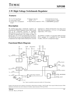
Suppose f is nonlinear, say f > 0. Assume that there exists two points x1 < x2 such
that
1
1
m1 = ′
< m2 = ′
.
f (u0 (x1 ))
f (u0 (x2 ))
Then the characteristics C1 = x1 (t) and C2 = x2 (t) drawn from the points (x1 , 0) and
(x2 , 0) respectively, have slopes m1 and m2 and intersect necessarily at some point P . At
this point P , the solution u will take both the values u0(x1 ) and u0 (x2 ), which is clearly
impossible if u is continuous. Hence, solution u can not be continuous at the point P .
Note that this phenomenon is independent of the smoothness of the functions u0 and f
t
P
C1
x1
C2
x
x2
Fig. 1.1
Example 2. Consider the Burgers equation
u2
ut +
2
1
with u(x, 0) = u0 (x) = 1 − x
0
if
if
if
!
=0
x
x<0
0≤x≤1
x>1
3
By using the method of characteristics, we can solve upto the time when the characteristics intersects. By (1.5) we have
x = x(x0 , t) = x0 + tu0 (x0 )
so that
x = x(x0 , t) =
x0 + t
x0 + t(1 − x0 )
x0
if
if
if
x0 ≤ 0
0 ≤ x0 ≤ 1
x0 ≥ 1
t
t=1
1
x
Fig. 1.2
For t < 1, the characteristics do not intersect. Hence given a point (x, t) with t < 1,
we draw the backward characteristic passing through this point, and we detemine the
corresponding x0 .
x0 =
x−t
if
if
if
x−t
1−t
x
1
1−x
1−t
⇒ u(x, t) =
0
u(x, 1) =
(
x≤t
t≤x≤1
x≥1
if
if
if
x≤t≤1
t≤x≤1
x ≥ 1, t < 1
At t = 1, the characteristics intersect. So we can say at t = 1,
1
0
if
if
x<1
x > 1.
Now it is clear that discontinuities may develop after a finite time if f is nonlinear, even
when u0 is smooth. These consideration lead us to introduce weak solutions.
4
1.2
Weak Solutions; Rankine-Hugoniot Condition:
Let v : IR × [0, ∞) → IR is a smooth function with compact support. Multiply (1.1) by
v and integration by parts:
0 =
∞
R R∞
0 −∞
= −
(ut + f (u)x )v dx dt
(1.7)
∞
R R∞
0 −∞
uvt dxdt −
∞
R ∞
R
0 −∞
f (u)vx dxdt −
∞
R
−∞
uv|t=0dx.
Now note that RHS of (1.7) is valid for any bounded measurable function u.
Definition: We say that u ∈ L∞ (IR×[0, ∞)) is a weak solution of (1.1) and (1.2) provided
Z∞ Z∞
(uvt + f (u)vx )dxdt +
0 −∞
Z∞
uv|t=0 = 0
(1.8)
−∞
for all smooth function v with compact support (usually v is called test function).
Suppose u satisfies (1.8) and u is smooth, then u satisfies (1.1). Solution of (1.8)
although not continuous, has a simple structure that we can see now.
Let x(t) be a curve in the (x, t) plane across which u(x, t) fails to be continuous, but
such that u has a limit as points (x, t) approaches the curve from either side. Suppose
in some openset V ⊂ IR × (0, ∞), u is smooth on either side of the smooth curve x(t).
Let Vl be the part of V on the left of the curve and Vr that part on the right. Assume u
and its first derivatives are uniformly continuous on Vl and Vr .
C = x(t)
t
V
l
Vr
x
Fig. 1.3
5
First choose a test function v with compact support in Vl . Then (1.8) become
0=
Z∞ Z∞
(uvt + f (u)vx )dxdt = −
0 −∞
Z∞ Z∞
(ut + f (u)x )v dxdt,
(1.9)
0 −∞
the integration by parts being justified since u is C 1 in Vl and v vanishes near the
boundary of Vl . The identity (1.9) holds for all test functions v with compact support in
Vl and so
ut + f (u)x = 0 in Vl .
(1.10)
ut + f (u)x = 0 in Vr
(1.11)
Similarly
Now choose a test function v with compact support in V but which does not necessarily
vanish along the curve x(t).
Again using (1.8) we have
0 =
=
Z∞ Z∞
(uvt + f (u)vx )dxdt
0 −∞
ZZ
(uvt + f (u)vx )dxdt
Vl ZZ
+
(uvt + f (u)vx )dxdt
Vr
Now since v has a compact support with in V , we have by (1.10)
ZZ
(uvt + f (u)vx )dxdt = −
Vl
ZZ
(ut + f (u)x )v dxdt
ZVl
+ (ul ν2 + f (ul )ν1 )v ds
Z
=
C
(ul ν2 + f (ul )ν1 )v ds
(1.12)
C
Here ν = (ν1 , ν2 ) is the unit normal to the curve C = x(t) pointing from Vl into Vr and
ul = lim u(x, t). Similalry
(x,t)→c
(x,t)∈Vl
ZZ
Vr
Z
(uvt + f (u)vx )dxdt = − (ur ν2 + f (ur )ν1 )v ds.
C
6
(1.13)
Here ur = lim u(x, t). By adding (1.12) and (1.13) we have
(x,t)→c
(x,t)∈Vr
Z
((f (ul ) − f (ur ))ν1 + (ul − ur )ν2 ) v ds = 0 along C.
C
We can take (ν1 , ν2 ) =
1
(1, −ẋ(t)).
(1+ẋ(t)2 )1/2
Hence
(f (ul ) − f (ur )) = ẋ(t)(ul − ur ) along the curve C = x(t).
(1.14)
Notation: [u] = ul − ur = jump in u across the curve C
[f (u)] = f (ul ) − f (ur ) = jump in f (u)
s = ẋ(t) = speed of the discontinuity .
Employing this notation we write (1.14) as
[f (u)] = s[u]
(1.15)
along the discontinuity curve. Relation (1.15) is called the Rankine-Hugnoit (R-H)
condition
Remark: Observe that the speed s = ẋ(t) and the values ul , ur f (ul ), f (ur ) will vary
along the curve C. The point is that even though these quantities change, the expression
[f (u)] = s[u] must always exactly balance.
Example 2’: Consider the same exaples 2. Observe that for t ≥ 1 the method of characterstics breaks down, since the characteristics intersects. Now we should define u for
t > 1 so that it satisfies the condition (1.15). Now solution
u(x, t) =
(
1
0
if
if
x<
x>
1+t
2
1+t
.
2
(1.16)
⇒
u(x, 1) =
(
1
0
if
if
x<1
x>1
and
1
ẋ(t) = s = ,
2
1
1
f (ul ) − f (ur ) = − 0 =
2
2
1
s(ul − ur ) =
2
⇒ solution (1.16) satisfies R-H condition along the curve C = x(t) =
7
1+t
.
2
+t
x = 1
2
t
u =1
u =0
1
t= 1
x
Fig. 1.4
Hence solution given by (1.16) is a weak solution for t ≥ 1.
Non-uniqueness of weak solutions: Let us now try the similar problem with
same techique.
Example 3 : Now consider the same Burgers equation
u2
ut +
2
with u(x, 0) =
(
0
1
if
if
!
=0
x
x<0
x > 0.
The method of characteristics this time does not lead to any ambiguity in defining
u, but does fail to give any information on the Wedge {0 < x < t}(see Fig.1.5).
t
? ?
u =1
u=0
x
Fig. 1. 5
Now how to fill up this gap? We can fill this gap in the fashion of previous exam-
8
ple(see Fig.1.6). Set
(
u1 (x, t) =
0
1
for
for
x < t/2
t/2 < x
t
t
x= _
2
u =1
u=0
x
Fig. 1.6
Along the curve C = x(t) = t/2,
f (ul ) − f (ur ) = 0 − 1/2, s = ẋ(t) = 1/2, ul − ur = 0 − 1 = −1.
Therefore u1 satisfies the R-H condition along C.
On the other hand we can fill this gap {0 < x < t} by(see Fig.1.7)
u2 (x, t) =
0
x
t
1
if
if
if
x<0
0<x≤t
x≥t
t
x =t
x
u= _
t
u =1
u=0
x
Fig. 1.7
9
Solution u2 is continuous and hence u2 is also a weak solution of the Burgers equation. Hence we need to find a criteria that enables us to choose the ”physically relevant
solution” among all the weak solutions of (1.1) and (1.2). Physically relevant solution: Let us look at the related viscous problem and will then let the viscosity tends to
zero. The viscous equation is
(
ut + f (u)x = ǫuxx
u(x, 0) = u0 (x)
(1.17)
Let uǫ (x, t) be the solution of (1.17) and u = lim u(x, t) in L1 -norm. Then u is a weak
ǫ→0
solution of (1.1) and (1.2). This u is called physically relevant solution of (1.1) and (1.2).
But how to pick up this physcially relevant solution. We want to find a simpler
condition. Fig.1.4 suggests that ’A shock should have characteristics going into the shock,
as time advances’.
A propagating discontinuity with characteristics coming out of it, as in Fig. 1.6, is
unstable to perturbations, i.e., if we add some viscosity to the system, will cause this to
be replaced by a rarefaction of characteristics as in Fig. 1.7. On this ground we like to
reject the solution u1 in Example 3. This gives us first version of Entropy Condition for
convex flux function f :
Entropy Condition (for convex flux function): A dicsontinuity propagating with a
speed s defined by (1.15) satisfies the entropy condition if
f ′ (ul ) > s > f ′ (ur ).
(1.18)
For a convex flux f , condition (1.18) is equivalent to
ul > ur
(1.19)
Now in Example 3, Solution u1 (x, t) not satisfying condition 1.18, hence we reject this
solution and keeping the continuous solution u2 .
A more general form of this condition, due to Oleinik, applies also to non convex
flux functions f :
Entropy condition (Oleinik) (for all flux functions): A discontinuity propogating
with a speed s defined by (1.15) satisfies the entropy condition if
f (v) − f (ur )
f (v) − f (ul )
≥s≥
.
v − ul
v − ur
10
(1.20)
b
f(u)
f(u)
ul
ur
ul
ur
u
u
Fig. 1.8
for all v between ul and ur .
If f is convex (1.20) reduces to (1.18).
The condition (1.20) has the simple geometric interpretation: f (u) must lie entirely
to one side of the chord joining (ul , (f ul )) and (ur , f (ur ))(see Fig.1.8). i.e., If ul < ur ,
then the graph of f over [ul , ur ] lies above the chord :
f (αur + (1 − α)ul ) ≥ αf (ur ) + (1 − α)f (ul ) for 0 ≤ α ≤ 1
(1.21)
If ur < ul , then the graph of f over [ur , ul ] lies below the chord :
f (αur + (1 − α)ul ) ≤ αf (ur ) + (1 − α)f (ul ) for 0 ≤ α ≤ 1
(1.22)
Also, Oleinik entropy condition is equivalent to the following Kruzkov entropy condition:
Kruzkov entropy condition: A weak solution u of (1.1) and (1.2) is the entropy
solution if
Z∞ Z∞ "
0 −∞
#
∂φ
∂φ
dxdt ≥ 0
+ sgn(u − l)(f (u) − f (l))
|u − l|
∂t
∂x
for all real l and for all non negetive smooth functions φ with compact support.
11
(1.23)
2
Riemann Problem
A conservation law together with piecewise constant data having a single discontinuity
is known as the Riemann Problem i.e.,
ut + f (u)x(= 0 in IR × (0, ∞)
Riemann Problem :
ul if x < 0
u(x, 0) =
ur if x > 0
(2.1)
Here ul , ur ∈ IR are the left and right initial states.
Riemann problem for convex flux:
Theorem 2.1(Solution of a Riemann problem for convex f ): Let f be strictly convex
and G = (f ′ )−1 .
(i) if ul > ur , then the weak solution satisfying entropy condition is given by
(
u(x, t) =
where s =
ul
ur
if
if
x < st
x > st
(2.2)
f (ul )−f (ur )
ul −ur
(ii) if ul < ur , then the weak solution satisfying entropy condition is given by
ul u(x, t) = G xt
u
r
x=st
u=ul
if
if
if
x < tf ′ (ul )
tf ′ (ul ) < x < tf ′ (ur )
x > tf ′ (ur )
t
u = ur
x
Fig. 2.1
12
(2.3)
' )
x =tf(u
l
t
x =tf'(ur)
x)
_
u = G(t
u = ur
u=ul
x
Fig. 2.2
Remark: In the first case the states ul and ur are separated by a shock wave with
constant speed s. In the second case the state ul and ur are separated by a (centered)
rarefaction wave.
Proof: (i) Across the shock u(x, t) satisfies the Rankine-Hugoniot condition. If x 6= st
the constant states ul and ur are the solution of left and right part of the shock. Since
ul > ur , the entropy condition holds as well.
(ii) it is enough to check that, solution defined in the region {f ′(ul ) < x/t < f ′ (ur )}
solves the equation in (2.1). Let u(x, t) = v(x/t). then
0 = ut + f (ux ) = ut +f ′ (u)u
x
1
x
′
′ x
′ x
·
+
f
(v)v
= −v
2
t
t
t t
1
x
x
[f ′ (v) − ]
= v′
t t
t
x
x
=
t
t x
x
′ −1 x
= (f )
=G
solves (3.1).
⇒ u(x, t) = v
t
t
t
′
⇒ f (v
Now v
x
t
= ul provided
x
t
= f ′ (ul ) and similarly v
x
t
= ur if
x
t
= f ′ (ur ).
⇒ Solutions defined in (2.3) is a continuous solution.
In the region {f ′ (ul ) <
x
t
< f ′ (ur )} solution satisfies
u(x + z, t) − u(x, t) = G(
13
x+z
x
)−G
t
t
≤ Lip(G)
z
t
for every z > 0. This shows solution defined (2.3) is a weak solution satisfying entropy
condition.
Riemann problem for general non canvex f : Let f be a non-convex function.
f(u)
ur
u*
ul
u
Fig. 2.3
Case (i): ul > ur (See Fig.2.3)
Consider the convex hull of the set
A = {(x, y)/ur ≤ x ≤ ul , y ≤ f (x)}.
(convex hull of the set A is the smallest convex set containing A). Look at the upper
boundary of the set, it is composed of straight line segment (ur , f (ur )) to (u∗ , f (u∗)) and
then y = f (x) upto (ul , f (ul )).
Connect ur to u∗ by a shock, u∗ can be calculated by
f ′ (u∗ ) =
f (u∗ ) − f (ur )
u∗ − ur
and then connect u∗ and ul by a rarefaction wave(see Fig.2.4).
Note that across the line x = tf ′ (ul ), solution is continuous and across the line
x = tf ′ (u∗ ), the solution is dicontinuous, with the left state u∗ and the right state ur
ul
u(x, t) = (f ′)−1 xt
u
r
x ≤ tf ′ (ul )
tf ′ (ul ) ≤ x ≤ tf ′ (u∗ )
x > tf ′ (u∗ ).
if
if
if
14
x= tf'(ul)
t
' *
x=tf(u )
u=G( x_
t)
u=ul
u=ur
x
Fig. 2.4
(f is a concave function in Fig.2.3 between u∗ and ul , hence G = (f ′ )−1 exists).
Case (ii): ul < ur (See Fig. 2.5)
In this case consider the convex hull of the set
A = {(x, y)/ul ≤ x ≤ ur , y ≥ f (x)}
f(u)
ul
u
*
ur
u
Fig. 2.5
Connect ul and u∗ by a rarefaction wave and then connect u∗ and ur by a shock
where u∗ is given by
f ′ (u∗ ) =
f (u∗ ) − f (ur )
u∗ − ur
.
15
See Fig.2.6
ul
u(x, t) = (f ′)−1 xt
u
r
x ≤ tf ′ (ul )
tf ′ (ul ) ≤ x ≤ f ′ (u∗ )t
x > tf ′ (ur )t.
if
if
if
x= tf'(ul)
t
'
x=tf(u*)
u=G( x_
t)
u=ul
u=ur
x
Fig. 2.6
3
Finite Differrence Schemes for Approximating Conservatin Laws
Here we restrict ourselves to explicit one step finite difference schemes. Descretize the
x−axis by a sequence {xi+ 1 } with xi+ 1 = (i + 12 )h, i ∈ Z, h > 0 and t−axis by {tn } with
2
2
tn = n∆t, n = 0, 1, 2, ..., ∆t > 0. ∆t and h are called time step and spacial mesh size
xi+ 1 +xi− 1
2
2
and
x
=
.
respectively. Let λ = ∆t
i
h
2
In order to approximate the conservation law
(
ut + f (u)x = 0 in IR × (0, ∞),
u(x, 0) = u0 (x), x ∈ IR
(3.1)
we introduce (2k + 1) point scheme of the form
n
n
n
n
vin+1 = H(vi−k
, vi−k+1
, ....., vin , ....., vi+k−1
, vi+k
)
(3.2)
where H : IR2k+1 → IR is a continuous function and vin denotes the approximation of the
exact solution u at the grid point (xi+ 1 , tn ). Initial data {vi0 } is defined by
2
vi0 =
1
h
Z
xi+ 1
2
xi− 1
u0 (x) dx.
2
16
(3.3)
If u0 (x) is continuous,then one can take
vi0 = u0i = u0 (xi ) ∀i
Definition: A difference scheme (3.2) is said to be in the conservative form,if there exists
a continuous function F : IR2k → IR such that
n
n
n
n
H(vi−k
, ..., vi+k
) = vin − λ(Fi+
1 − F
i− 1 )
2
2
(3.4)
n
n
n
where Fi+
1 = F (vi−k+1 , ..., vi+k ). The function F is called numerical flux.
2
Definition: The diffrence scheme (3.4) is said to be consistence with the equation (3.1)
if
F (v, ..., v) = f (v) ∀v ∈ IR
(3.5)
H(v, ..., v) = v ∀v ∈ IR
(3.6)
i.e.,
In order to analyze the convergence of the solution {vin } of the difference scheme
(3.4) we introduce the piecewise constant function vh defined a.e. in IR × (0, ∞) by
vh (x, t) = vin for (x, t) ∈ (xi− 1 , xi+ 1 ) × [tn , tn+1 )
2
2
(3.7)
Theorem 4.1 (Lax-Wendroff)Let vh be the numerical solution obtained from the scheme
(3.2) which is in the conservative form and consisitent with equation (3.1). Assume that
there exists a sequence {hk } which tends to 0 as k → ∞ such that,if we set ∆k t = λhk
(λ = ∆hkkt , kept constant)
(i)||vhk ||L∞ (IR×(0,∞)) ≤ C for some constant C > 0,
(ii) vhk converges in L1loc (IR × (0, ∞)) and a.e to a function v. Then v is a weak solution
of (3.1).
Proof: Let φ ∈ C01 (IR × IR+ ) and let
φni = φ(xi , tn ),
φh (x, t) = φni
Multiply equation (3.4) by
h
if
φni
(x, t) ∈ [xi− 1 , xi+ 1 ) × [n∆t, (n + 1)∆t).
i,n
2
and sum it over i and n,then we have
(vin+1 − vin )φni + ∆t
X
2
X
n
n
n
(Fi+
1 − F
i− 1 )φi = 0.
i,n
17
2
2
A summation by parts gives
h
X
u0i φ0i + h
X
vin+1 (φn+1
− φni ) + ∆t
i
Fi+ 1 (φni+1 − φni ) = 0.
i,n
i,n
i
X
2
Now define a piecewise constant function Fh by
n
n
n
Fh (x, t) = Fi+
1 = F (vi−k+1 , ..., vi+k ), (x, t) ∈ (xi , xi+1 ) × [tn , tn+1 )
2
Now since vh is bounded in L∞ (IR × (0, ∞)) we have
h
X
vi0 φ0i
=
i
Z
vh (x, 0)φh (x, 0)dx
Z
vh (x, 0)φ(x, 0)dx + O(h)
IR
=
(3.8)
IR
h
X
vin+1 (φn+1
i
−
φni )
=
i,n
=
Z∞ Z∞
∆t −∞
Z∞ Z∞
vh (x, t)
φh (x, t) − φh (x, t − ∆t)
dxdt
∆t
vh (x, t)
∂φ
dxdt + O(h),
∂t
∆t −∞
∆t
X
i,n
Fi+ 1 (φni+1
2
−
φni )
=
Z∞ Z∞
Fh (x, t)
φh (x + h, t) − φh (x, t)
dxdt
h
=
Z∞ Z∞
Fh (x, t)
∂φ
dxdt + O(h).
∂x
0 −∞
0 −∞
Observe first that
1
1
Fh (x, t) = F (vh (x − (k − )h, t), ..., vh (x + (k − )h, t))
2
2
and set
1
whi (x, t) = vh (x + (i − )h, t), −k ≤ i ≤ k.
2
Let K be a compact subset of IR × (0, ∞) and K1 = K + (i − 12 )h. Then
Z
K
|whi (x, t)
− v(x, t)| dx dt ≤
Z
|vh (x, t) − v(x, t)| dx dt
K1
+
Z
K
18
1
|v(x + (i − )h, t) − v(x, t)| dx dt
2
(3.9)
(3.10)
In the right side of the above inequality first term goes to 0 because vh converges to v in
L1loc and the second term goes to 0 by the property, continuity in mean of the function
v. Therefore whi converges to v in L1 (K) for all |i| ≤ k. Therfore we can exract a
subsequence ,still denoted by whi ,which converges to v a.e in K. Since F is continuous
we have,
Fh (x, t) = F (wh−k+1(x, t), ..., whk (x, t)) → F (v(x, t), ..., v(x, t))
a.e in K. Hence by consistency property (3.6), F (v, .., v) = f (v). It follows from Lebesgue
dominated convergence theorem we have
Z∞ Z∞
0 −∞
∂φ
Fh (x, t) dxdt →
∂x
Z∞ Z∞
f (v((x, t))
0 −∞
∂φ
dxdt
∂x
. Since vh converges to v in L1loc (IR × (0, ∞)), then from (3.8) and (3.9),finally (3.8)
gives(by going to further subsequence hk , if necessary)
Z∞
u0 φ(x, 0)dx +
Z∞ Z∞
0 −∞
−∞
Z∞ Z∞
∂φ
∂φ
f (v) dxdt = 0
v dxdt +
∂t
∂x
0 −∞
∀ φ ∈ C01 (IR × IR+ ).
⇒ v is a weak solution of (3.1).
Examples of 3-point scheme:
The entropy solution of the Riemann problem
ut + f (u)x(= 0 in IR × (0, ∞)
ul if x < 0
u(x, 0) =
ur if x > 0
(3.11)
is self-similiar,i.e., of the form
x
u(x, t) = wR ( , ul , ur )
t
(3.12)
where wR depends only on the function f and consists of two constant states ul and
ur . Now observe that ξ → f (wR (ξ, ul , ur )) is a continuous function at ξ = 0. Indeed
if wR (ξ, ul , ur ) is discontinuous at ξ = 0,this means that this discontinuity is stationary(the corresponding discontinuous wave moves with zero speed). Hence by RankineHugoniot condition and continuity of f (wR (ξ, ul , ur )) at ξ = 0 we have
f (wR (0−, ul , ur )) = f (wR (0+, ul , ur )) = f (wR (0, ul , ur ))
19
(3.13)
Example 3.1:The Godunov scheme:
Step-1: First we would like to solve exactly the following problem with piecewise constant initial data:
(
wt + f (w)x = 0, t ∈ (tn , tn+1 ]
w(x, tn ) = vh (x, tn )
(3.14)
where vh (x, tn ) = vin , x ∈ (xi− 1 , xi+ 1 )∀i ∈ Z. To solve this we decompose this problem
2
2
into several local Riemann problem centered at points xi+ 1 ,for each i ∈ Z i.e.,
2
wt + f (w)x(= 0, t ∈ (tn , tn+1 ]
vin
if x < 0
w(x,
t
)
=
n
n
vi+1
if x > 0
Let
(3.15)
1
λ sup |f ′ (vj )| ≤ .
2
vj
(3.16)
The condition like (3.16) is called Courant-Friedrichs-Lewy(CFL) condition. Then waves
from two neighbouring Riemann problems do not intersect before time ∆t. Infact (3.16)
ensures that a wave from xi+ 1 will not reach the linex = xi and x = xi+1 before time ∆t.
2
Hence problem (3.14) can be seen as a superposition of local Riemann problems
under the condition (3.16). The solution of (3.14) in (xi , xi+1 ) × (tn , tn+1 ] is given by
n
w(x, t) = wR ((x − xi+ 1 )/t − tn , vin , vi+1
), x ∈ (xi , xi+1 ), t ∈ (tn , tn+1 ].
2
Now solution at t = tn+1 is given by
n
w(x, tn+1 ) = wR ((x − xi+ 1 )/∆t, vin , vi+1
), x ∈ (xi , xi+1 )
2
Step 2: Define vin+1 by
vin+1 =
1
h
=
Z
xi
Z
0
Z
xi+ 1
2
xi− 1
2
xi− 1
=
w(x, tn+1 ) dx
wR ((x −
n
xi− 1 )/∆t, vi−1
, vin ) dx
2
2
−h
2
n
wR (x/∆t, vi−1
, vin ) dx +
Z
0
h
2
+
Z
xi+ 1
xi
2
n
) dx
wR ((x − xi+ 1 )/∆t, vin , vi+1
2
n
wR (x/∆t, vin , vi+1
) dx
In order to get a simple expression for vin+1 , integrate the equation (3.14) over the cell
(xi− 1 , xi+ 1 ) × (tn , tn+1 ),then we have
2
2
0 =
Z
tn+1
tn
Z
xi+ 1
2
xi− 1
(wt + f (w)x ) dx dt
2
20
=
Z
xi+ 1
2
xi− 1
+
=
w(x, tn+1 ) dx −
Z2 tn+1
tn
h(vin+1
Z
xi+ 1
2
xi− 1
w(x, tn ) dx
2
f (w(xi+ 1 − 0, t) dt +
2
Z
tn+1
tn
f (w(xi− 1 + 0, t) dt
2
n
n
− vin ) + ∆t(f (wR (0−, vin , vi+1
)) − f (wR (0+, vi−1
, vin )))
But by (3.13),
n
n
n
f (wR (0−, vin , vi+1
)) = f (wR (0+, vin , vi+1
)) = f (wR (0, vin , vi+1
))
Now Godunov scheme is given by
n
n
vin+1 = vin − λ(Fi+
1 − F
i− 1 )
2
(3.17)
2
where its numerical flux
G n n
n n
n
Fi+
1 = F (vi , vi+1 ) = f (wR (0, vi , vi+1 )).
2
Godunov has given the following simple formula for a general f to evaluate the numerical
flux
F G (u, v) = (
f (wR (0, u, v))
minw∈[u,v] f (w)
=
maxw∈[v,u] f (w)
if
if
u≤v
u≥v
(3.18)
Godunov scheme (3.17) is in conservative form, consistent with the conservation law
(3.1) and also an upwind scheme i.e.,
G
F (u, v) =
(
f (u) if f is a nondecreasing function between u and v
f (v) if f is a nonincreasing function between u and v
Remark: If f is a convex function and f (θ) = minw∈IR f (w),then the Godunov flux
(3.18) can be expressed in more simpler form
F G (u, v) = max(f (max(u, θ)), f (min(v, θ))).
Similarly if f is concave and f (θ) = maxw∈IR f (w),then
F G (u, v) = min(f (min(u, θ)), f (max(v, θ))).
n
Remark: As Godunov flux Fi+
1 depends on the solution of Riemann problem at x =
2
xi+12 only and the waves from x = xi+ 1 does not reach x = xi− 1 and x = xi+ 3 in time
2
2
2
∆t, we can relax the codition (3.16) by
λ sup |f ′ (vj )| ≤ 1
vj
21
(3.19)
Example 3.2. The Lax-Friedrichs scheme:
This is the simplest centered finite scheme which is given by
λ
n
n
) − f (vi−1
))
vin+1 = vin − (f (vi+1
2
n
n
n
= vi − λ(Fi+ 1 − Fi− 1 )
2
2
(3.20)
where
1
1 n
n
LF
n
n
Fi+
(vin , vi+1
) = (f (vin ) + f (vi+1
) − (vi+1
− vin ))
1 = F
2
2
λ
This is in a conservative form and is consistent with conservation law (3.1) but is not an
upwind scheme. However this scheme can be interpreted as a projection of the solution
n
n
i
, vi−1
, vi+1
) be
of successive non-interacting Riemann problems. Let w(x, t) = wR ( x−x
t
the solution of Riemann problem
wt + f (w)x(= 0, t ∈ (tn , tn+1 ]
n
vi−1
if x < xi
w(x, tn ) =
n
vi+1 if x > xi
where
(3.21)
xi+ 1 + xi− 1
2
∀i ∈ Z.
2
Here we consider Riemann problems centered at x = ..., xi−4 , xi−2 , xi , xi+2i , ... so that the
waves from nighbouring cells does not interact. Observe that under the CFL condition
xi =
2
n
(3.16),the solution of (3.21) w(x, t) satisfies, w(xi−1 + 0, t) = vi−1
and w(xi+1 − 0, t) =
n
vi+1 ∀t ∈ (tn , tn+1 ). Define
vin+1
=
Z
xi+1
xi−1
wR (
x − xi n
n
, vi−1 , vi+1
)
∆t
Like in the derivation of Godunove scheme,by integrating over the rectangle (xi−1 , xi+1 )×
(tn , tn+1 ) we have
0 =
=
Z
tn+1
Ztnxi+1
xi−1
+
Z
Z
xi+1
xi−1
w(x, tn+1 ) dx −
tn+1
tn
(wt + f (w)x ) dx dt
Z
xi+1
xi−1
w(x, tn ) dx
f (w(xi+1 − 0, t) dt +
= 2h(vin+1 −
Z
tn+1
tn
f (w(xi−1 + 0, t) dt
n
n
vi−1
+ vi+1
n
n
) + ∆t(f (vi+1
)) − f (vi−1
)))
2
This is Lax-Friedrichs scheme.
22
Example 3.3. The Murman-Roe scheme:
Define
a(u, v) =
(
(f (u)−f (v))
u−v
′
f (u)
if u 6= v
if u = v
(3.22)
We proceed as in the Godunov scheme,only replacing the local Riemanproblem (3.15) by
that of linear problem
The solution of (3.23),
w(x, t) =
Roe
wR
(
n
wt + a(vin , vi+1
)w = 0,
( n x
vi
if x < xi+ 1
2
w(x, tn ) =
n
vi+1 if x > xi+ 1
(3.23)
2
x − xi+ 1
2
t
n
, vin , vi+1
)
=
(
n
)t
if x − xi+ 1 < a(vin , vi+1
2
n n
if x − xi+ 1 > a(vi , vi+1 )t
vin
n
vi+1
(3.24)
2
n
has a discontinuity moving with a speed a(vin , vi+1
).
Exactly like in the construction of Godunov scheme,we have Murman-Roe scheme
n
n
vin+1 = vin − λ(Fi+
1 − F
i− 1 )
2
2
(3.25)
where
Roe n n
Roe
n
n
(vi , vi+1 ) = f (wR
(0, vin , vi+1
)).
Fi+
1 = F
2
This flux can be written further in the following form
1
F Roe (u, v) = (f (u) + f (v) − |a(u, v)|(v − u))
2
Murman-Roe scheme is in conservative form,consistent with the conservation law
(3.1) and also an upwind scheme.
Example 3.4. The Engquist-Osher scheme:
Engquist-Osher scheme is given by
n
n
vin+1 = vin − λ(Fi+
1 − F
i− 1 )
2
2
(3.26)
n
EO n n
where the numerical flux Fi+
(vi , vi+1 ) and
1 = F
2
1
F EO (u, v) = (f (u) + f (v) −
2
23
Z
v
u
|f ′ (ξ)| dξ)
(3.27)
Enguist-Osher scheme is in conservative form,consistent with the conservation law
(3.1) and also an upwind scheme.
Remark: if f is a convex function and f (θ) = minw∈IR f (w),then the Engquist-Osher
flux (3.27) can be expressed in more simpler form
F EO (u, v) = f (max(u, θ)) + f (min(v, θ)) − f (θ)
. Similarly if f is concave and f (θ) = maxw∈IR f (w),then
F EO (u, v) = f (min(u, θ)) + f (max(v, θ)) − f (θ)
.
Example 3.5. The Lax-Wendroff scheme:
This scheme is derived by a Taylor series expansion of a smooth solution of (3.1),where
the term of order strictly greater than two are neglected,thus leading to a second order
scheme. Let u be a smooth solution of (3.1),then we have
u(x, t + ∆t) = u(x, t) + ∆t ut (x, t) + (∆t2 /2) utt (x, t) + 0(∆t3 )
= u(x, t) − ∆t f (u)x + (∆t2 /2) + (f ′ (u)(f (u)x )x + 0(∆t3 )
Now
f (u(x + h, t)) − f (u(x − h, t))
+ o(h2 )
f (u)x =
2h
(f ′ (u)(f ((u)x)x = [f ′ ((u(x + h, t) + u(x, t))/2)(f (u(x + h, t) − f (u(x, t)))−
f ′ ((u(x, t) + u(x − h, t))/2)(f (u(x, t) − f (u(x − h, t)))]/h2 + o(h).
This leads to the following Lax-Wendroff scheme
n
n
vin+1 = vin − λ(Fi+
1 − F
i− 1 )
2
2
(3.28)
LW
n
n
(vin , vi+1
) and
where the numerical flux Fi+
1 = F
2
u+v
1
)(f (v) − f (u)))
F LW (u, v) = (f (u) + f (v) − λ f ′ (
2
2
(3.29)
Lax-Wendroff scheme is in conservative form,consistent with the conservation law
(3.1) and but not an upwind scheme
24
3.1
Monotone and TVD Schemes
Definition: The finite difference scheme (3.2) is said to be monotone if H is non
decreasing function of each of its arguments.
Notation: Let v = (vi )i∈Z and w = (wi )i∈Z then v ≥ w means vi ≥ wi ∀i ∈ Z.
Let (H∆ (v))i = H(vi−k , vi−k+1 , ....., vi , ....., vi+k−1 , vi+k ) and H∆ (v) = (H∆ (v))i )i∈Z
then scheme (3.2) is monotone means,
v ≥ w ⇒ H∆ (v) ≥ H∆ (w)
Examples of monotone schemes: Godunov,Lax-Friedrichs and Enquist-Osher schemes
are monotone under the CFL like condition
λ sup |f ′(vj )| ≤ 1.
vj
(3.30)
Proposition 3.2: If a 3-point scheme which is in conservative form and is monotone,then
the numerical flux F (u, v) is an incrasing function in its first argumennt,and a decreasing
function in its second argument.
Proof: By the definition of a 3-point conservative scheme,
H(v−1 , v0 , v1 ) = v0 − λ(F (v0 , v1 ) − F (v−1 , v0 )).
Thus the mapping
u → F (u, v0) =
1
[H(u, v0, v1 ) − v0 ] + F (v0 , v1 )
λ
is increasing iff u → H(u, v0, v1 ) is increasing and
1
v → F (v0 , v) = − [H(v−1 , v0 , v) − v0 ] + F (v−1 , v0 )
λ
is decreasing iff u → H(v−1 , v0 , v) is increasing.
Converse of Proposition 3.2:
Suppose F(u,v) is increasing in its first argument and decreasing in second argument,then
the scheme is monotone provided,
λ max
{|F (u, w) − F (v, w)| + |F (z, u) − F (z, v)|} ≤ |u − v| ∀u, v.
w,z
25
Given a sequence v = (vi )i∈Z we define the following norms
||v||1 = h
X
|vi |
(3.31)
||v||∞ = max |vi |
(3.32)
X
(3.33)
i∈Z
i∈Z
T V (v) =
|vi+1 − vi |
i∈Z
Lemma 3.3. (Crandall-Tartar): Let (Ω, µ) be a mesure space and C be a subset of
L1 (Ω) such that
f, g ∈ C ⇒ max(f, g) ∈ C
Let T be a mapping from C to L1 (Ω) which satisfies
Z
Ω
T (f ) dµ =
Z
Ω
f dµ ∀f ∈ C.
(3.34)
Then the following properties are equivalent:
(a) T is order preserving i.e.,
f, g ∈ C and f ≤ g a.e ⇒ T (f ) ≤ T (g) a.e
(b)
Z
Ω
(c)
Z
|T (f ) − T (g)|+ dµ ≤
Z
|f − g|+ dµ
|T (f ) − T (g)| dµ ≤
Z
|f − g| dµ
Ω
Ω
Ω
∀f, g ∈ C.
∀f, g ∈ C.
Proof: (a) ⇒ (b):
Since max(f, g) = g + (f − g)+ ,by the property (a) we have
T (max(f, g)) ≥ T (g)
and similarly
T (max(f, g)) ≥ T (f )
By subtracting T (g) from both the sides of above inequalities,we get
T (max(f, g)) − T (g) ≥ (T (f ) − T (g))+
26
Integrate over Ω the above inequality,we get
Z
Ω
(T (f ) − T (g))+ dµ ≤
=
=
Z
ZΩ
ZΩ
Ω
(T (max(f, g)) − T (g)) dµ
(max(f, g) − g) dµ by (3.34)
(f − g)+ dµ
(b) ⇒ (c):
Using the identity
|f − g| = (f − g)+ + (g − f )+
we have
Z
Ω
Z
|T (f ) − T (g)| dµ =
ZΩ
≤
ZΩ
=
(c) ⇒ (a):
Since (f − g)+ =
Z
Ω
1
(|f
2
Ω
(T (f ) − T (g))+ dµ +
(f − g)+ dµ +
|f − g| dµ
Z
Ω
Z
Ω
(T (g) − T (f ))+ dµ
(g − f ))+ dµ
− g| + (f − g)) and by the property (3.34),we get
1
(|T (f ) − T (g)| + (T (f ) − T (g))) dµ
2 ZΩ
1
(|f − g| + (f − g)) dµ
≤
Z2 Ω
=
(f − g)+
(T (f ) − T (g))+ dµ =
Z
Ω
Suppose f ≤ g a.e,then (f − g)+ = 0 a.e,hence we get
Z
Ω
(T (f ) − T (g))+ dµ ≤ 0
which implies T (f ) ≤ T (g) a.e. This completes the proof of Lemma 3.3.
Lemma 3.4.(l∞ stability): Let v n = (vin )i∈Z ∈ l∞ and scheme (3.4) is monotone,
consistent,then v n+1 = (vin+1 )i∈Z ∈ l∞ and
||v n+1 ||∞ ≤ ||v n ||∞
(3.35)
Proof: Since H is increasing in each of its arguments,we have
min
i−k≤j≤i+k
n
n
{vjn } ≤ H(vi−k
, ..., vi+k
)≤
27
max {vjn }
i−k≤j≤i+k
. Let
|vm | =
max {|vln |}.
i−k≤l≤i+k
Then by consisstency and monotonicity of the scheme we, have
n
n
−|vm | = H(−|vm |, −|vm |, ..., −|vm |) ≤ H(vi−k
, ..., vi+k
) ≤ H(|vm |, |vm |, ..., |vm |) = |vm |.
Hence we have
|vin+1| ≤ |vm | =
max {|vln |}.
(3.36)
i−k≤l≤i+k
This implies the result.
Let
v n+1 = H∆ (v n ) = ((H∆ (v n ))i )i∈Z
and
n
n
(H∆ (v n ))i = H(vi−k
, ..., vi+k
) = vin+1 .
Lemma 3.5(l1 contraction) Suppose v n ∈ l∞ and the scheme (3.2) is in conservative
form,consistent and monotone. Then H∆ : l1 → l1 is a mapping which preserves the
integral and for any sequence u and v in l1 we have
||H∆ (u) − H∆ (v)||1 ≤ ||u − v||1
(3.37)
Proof:(a) From (3.36) we have
|(H∆ (v n ))i | ≤
max {|vln |} ≤
i−k≤l≤i+k
i+k
X
|vln |.
l=i−k
By taking summation over i and multiplying by h we get
h
X
|(H∆ (v n ))i | ≤≤ (2k + 1)h
i∈Z
X
|vln |.
i∈Z
⇒ v n+1 ∈ l1
.
(b) By taking summation over i and multiplying by h in (3.4) we get
h
X
vin+1 = h
i∈Z
X
i∈Z
Hence H∆ preserves the integral.
28
vin .
(c) H∆ is order preserving follows from scheme is monotone. Hence by Crandall and
Tartar lemma we have
||H∆ (u) − H∆ (v)||1 ≤ ||u − v||1
i.e.,
h
X
|un+1
− vin+1 | = h
i
i∈Z
X
|uni − vin |.
i∈Z
Definition: A scheme is said to be total variation diminishing(TVD) if
T V (v n+1 ) ≤ T V (v n ) ∀n = 0, 1, 2, ....
Lemma 3.6(TVD): Any conservative,consistent monotone scheme satisfies total variation diminishing property i.e.,
X
n+1
|vin+1 − v1−1
| =
i∈Z
X
n
|vin − vi−1
|.
i∈Z
i.e.,
T v(v n+1) ≤ T V (v n )
(3.38)
n
Proof: By taking uni = vi−1
in (3.37),we get (3.38).
Lemma 3,7.(Time estimate): Let scheme (3.2) be in conservative form, consistent
with (3.1) and TVD with a Lipschitz continuous numerical flux Fi+ 1 . Assume moreover
2
that scheme is l∞ stable. Then there exists a constant C > 0 such that ∀ 0 ≤ m ≤ n,
h
X
|vim − vin | ≤ C(m − n)∆tT V (v 0 )
(3.39)
i∈Z
Proof: From (3.4) we have,
vin+1 − vin = λ(Fi+ 1 − Fi− 1 )
2
2
and since F is lipschitz continuous,there exists a constant c1 = c1 (F, ||v 0||∞ ) > 0 such
that for C = 2kc1 , n > m,
n−1
n−1
n−1
n−1
|vin − vin−1 | ≤ λc1 {|vi−k+1
− vi−k
| + ..., |vi+k
− vi+k−1
|
≤ 2kc1 T V (v n−1 )
≤ CT V (v m )
29
Since scheme is TVD and
|vin − vim | ≤ |vin − vin−1 | + |vin−1 − vin−2 | + ... + |vim+1 − vim |
then we get by taking summation over i and multiplying by h,
h
X
|vin − vim | ≤ C(m − n)∆tT V (v m ).
i∈Z
This completes the proof.
Let vh defined by (3.7) be the piecewise constant function i.e.,
vh (x, t) = vin for (x, t) ∈ (xi− 1 , xi+ 1 ) × [tn , tn+1 )
2
2
(3.40)
Let 0 ≤ s ≤ t ≤ T for any T > 0. Let tn , tm be such that tm ≤ s < tm+1 and
tn ≤ t < tn+1 . Then
|tn − tm | ≤ |t − s| + ∆t
and
vh (., t) − vh (., s) = vh (., tn ) − vh (., tm )
Then under the assumption of Lemma 3.7 we have
||vh (., t) − vh (., s)||L1 ≤ C(|t − s| + ∆t)T V (vh (., 0)
(3.41)
for some constant C > 0, 0 ≤ s ≤ t ≤ T . Here C is independent of t. Equation (3.41)
says that vh is Lipschitz continuous in t w.r.t L1 norm.
Now we state the final result for convergence.
Theorem 3.8(Existence of a weak solution): Let for any T > 0,
(a) u0 ∈ L∞ (IR) and BV (IR),a functions of bounded variations and v 0 given by (3.3).
(b) vh (x, t) be an approximate solution obtained from a difference scheme (3.2) which is
in conservative form and consistent with (3.1).
(c) ||vh (., t)||∞ < ∞ and a T V (vh (., t)) < ∞ for 0 ≤ t ≤ T .
(d)
||vh (., t) − vh (., s)||L1 ≤ C(|t − s| + ∆t)T V (vh (., 0)
for some constant C > 0, 0 ≤ s ≤ t ≤ T.
Then there exists a sequence hk → 0 such that if we set,∆k t = λh,with λ being
kept constant,the sequence vhk converges in L∞ (0, T ; L1loc (IR)) , say to u. This limit u is
30
a weak solution of (3.1).
Proof: Let Ω be a bounded openset in IR. By (a) and (b) vh (., t) ∈ BV (Ω) as well as in
L1 (Ω) for any 0 ≤ t ≤ T .
Let (sn )∞
n=0 be a countable dense subset of [0, T ]. Since the canonical embedding
BV (Ω) in L1 (Ω) is compact for any bounded set of Ω, then for each sk there exists a
subsequence hk of h → 0 such that vhk (·, sk ) coverges ,say to u(·, sk ) in L1loc (IR). Again
by a diagonalisation argument we find another subsequence of hk still denoted by hk such
that vhk (·, sj ) → u(·, sj ) for all j. In order to reach every point t in [0, T ],we partition the
interval [0, T ] into N intervals (ti , ti+1 ) where ti are selected from the dense set (sn )∞
n=0 in
such a way that each interval has length less than ǫ > 0, where ǫ is any given arbitrary
positive constant. For any t ∈ [0, T ] there exists ti such that |t − ti | ≤ ǫ and
||vhk (·, t) − vhm (·, t)||L1 (Ω) ≤ ||vhk (·, t) − vhk (·, ti )||L1 (Ω) + ||vhk (·, ti ) − vhm (·, ti )||L1 (Ω) +
||vhm (·, ti ) − vhm (·, t)||L1(Ω)
By (d),there exists a constant C independent of t such that first and the last
term are bounded by C(∆t + ǫ). The term in the middle can be made less than ǫ by
the fact that vhk (·, sj ) → u(·, sj ) for all j in L1loc (IR). Hence uhk (·, t) is a uniform in
t ∈ [0, T ] cauchy sequence in L1loc (IR). Therefore we can extract a subsequence hk → 0
such taht vhk converges in L∞ (0, T ; L1loc(R)) say to u(·, t) and almost everywhere. From
this we can conclude that there exists a subsequence hk → 0 such that vhk converges
in L1loc (IR × (0, ∞)) and a.e to a function u. By Lax-Wendroff’s theorem u is a weak
solution of conservation law (3.1). This completes the proof of theorem.
31
Descretized version of Kruzkov’s entropy condition (1.23):
Now we show that monotone scheme satisfies the descretized version of the Kruzkov
entropy condition:
|un+1
− l| − |uni − l| + λ(Gni+1/2 − Gni−1/2 ) ≤ 0
i
n
n
for any real number l, where Gni+1/2 = G(vi−k+1
, ..., vin , ..., vi+k
) is such that
G(u, u) = sgn(u − l)(f (u) − f (l)).
(3.42)
Consider a monotone scheme which is in conservation form and consistent with
(3.1):
n
n
vin+1 = H(vi−k
, ..., vin , ..., vi+k
)
n
n
vin − λ(Fi+1/2
− Fi−1/2
)
(3.43)
n
n
n
where H is non-decreasing in each of its arguments and Fi+1/2
= F (vi−k+1
, ..., vin , ..., vi+k
)
with F (v, v, ..., v, v) = f (v). Set a ∨ b = max(a, b) and a ∧ b = min(a, b). Define
n
n
n
n
n
n
G(vi−k+1
, ..., vi+k
) = F (vi−k+1
∨ l, ..., vi+k
∨ l) − F (vi−k+1
∧ l, ..., vi+k
∧ l).
Then G(v, ..., v) = sgn(v − l)(f (v) − f (l)) satisfies the condition (3.42).
Consider
−λ(Gi+1/2 − Gi−1/2 ) = −λ(F (vi−k+1 ∨ l, ..., vi+k ∨ l) − F (vi−k ∨ l, vi+k−1 ∨ l))
+λ(F (vi−k+1 ∧ l, ..., vi+k , ∧l) − F (vi−k ∧ l, ..., vi+k−1 ∧ l))
= H(vi−k ∨ l, ..., vi ∨ l, ..., vi+k ∨ l) − vi ∨ l
−H(vi−k ∧ l, ..., vi ∧ l, ..., vi+k ∧ l) + vi ∧ l
⇒
|vi −l|−λ(Gi+1/2 −Gi−1/2 ) = H(vi−k ∨l, ..., vi ∨l, ..., vi+k ∨l)−H(vi−k ∧l, ..., vi ∧l, vi+k ∧l).
Note that
n
n
n
n
H(vi−k
∨ l, ..., vin ∨ l, ..., vi+k
∨ l) ≥ H(vi−k
, ..., vin , ..., vi+k
) ∨ H(l, l, l)
32
= vin+1 ∨ l
Similarly
n
n
n
n
H(vi−k
∧ l, ..., vin ∧ l, ..., vi+k
∧ l) ≤ H(vi−k
, ..., vin , ..., vi+k
) ∧ H(l, l, l)
= vin+1 ∧ l
⇒
|vin+1 − l| − |vin − l| + λ(Gni+1/2 − Gni−1/2 ) ≤ 0
Corollary 3.9.: Solution obtained from a consistent,conservative monotone scheme converges to the entropy solution of (3.1).
Proof: solution obtained from any consistent,conservative monotone scheme satisfies the hypothesis of theorem 3.8, hence there exists a subsequence hk such that vhk
converges in L∞ (0, T ; L1loc (IR)) say to u. Since approximate solution obtained from monotone scheme satisfies the descrete entropy condition,by uniqueness, all the subsequence
of vhk converges to u only. This implies whole sequence vh converges to u. This u is a
weak solution and satisfies the entropy condition.
Example of scheme which converges to weak solution but not to entropy
solution:
Consider a Murman-Roe scheme for the following Riemann problem:
2
ut + ( u2 )x(= 0 in IR × (0, ∞)
−1 if x < 0
u(x, 0) =
1
if x > 0
(3.44)
Then we have vin+1 = vin ∀i ∈ Z. This scheme admits entropy violating stationary
shocks. Hence this is not a monotone scheme.
One of the important criteria to establish the convergence of the scheme is total
variation bound. In the next section we give general criteria which ensures the scheme
is TVD. Monotone schemes obviously satisfies this criteria.
33
3.2
Incremental form and Numerical viscosity
Definition : A scheme is said to be in an incremental form if there exists functions
C, D called incremental coefficients such that
vin+1 = vin − Ci− 1 ∆vi− 1 + Di+ 1 ∆vi+ 1
2
2
2
(3.45)
2
n
n
) and Di+ 1 = D(vin , vi+1
).
where ∆vi+ 1 = vi+1 − vi , Ci+ 1 = C(vin , vi+1
2
2
2
Example: Any consistent,conservative scheme (3.4) with Lipschitz continuous flux admits a unique incremental form with incremental coefficients given by
n
n
n
n
Ci+
= λ(f (vi+1
) − Fi+
1
1 )/∆v
i+ 12
2
2
and
n
n
n
= λ(f (vin ) − Fi+
Di+
1 )/∆v
1
i+ 1
2
2
(3.46)
2
n n
n
where Fi+
1 = F (vi , vi+1 ).
2
Definition : A scheme is said to be in viscous form if there exists a function Q called
n
the coefficient of numerical viscosity such that if we set Qni+ 1 = Q(vin , vi+1
) the scheme
2
can be written
1
λ
n
n
n
n
n
) − f (vi−1
)) + (Qni+ 1 ∆vi+
vin+1 = vin − (f (vi+1
1 − Q
i− 21 ∆vi− 12 ).
2
2
2
2
(3.47)
Any 3-point scheme with Lipschitz numerical flux admits a unique viscous form whose
numerical viscosity coefficient is given by
Qi+ 1 = λ(f (vi ) + f (vi+1 ) − 2Fi+ 1 )/∆vi+ 1
2
2
.
Moreover,
Qi+ 1 = Ci+ 1 + Di+ 1
2
Ci+ 1 =
2
and
Di+ 1 =
2
2
2
Qi+ 1
λ f (vi+1 ) − f (vi )
2
(
)+
2
vi+1 − vi
2
Qi+ 1
−λ f (vi+1 ) − f (vi )
2
)+
(
.
2
vi+1 − vi
2
34
2
where Ci+ 1 , Di+ 1 are the unique incremental coefficients defined by (3.46). Note
2
2
)−f (vi )
|
that Ci+ 1 ≥ 0 and Di+ 1 ≥ 0 iff Qi+ 1 ≥ λ| f (vvi+1
i+1 −vi
2
2
2
For example,Coefficient of numerical viscosty of Lax-Friedrichs,Enguist-Osherand
Murman-Roe schemes are given by
= 1,
(a) Lax-Friedrichs scheme,Qi+ 1 = QLF
i+ 1
2
2
=λ
(b) Engquist-Osher scheme, Qi+ 1 = QEO
i+ 1
2
2
=
(c) Murman-Roe scheme Qi+ 1 = QRoe
i+ 1
2
2
n
R vi+1
|f ′ (ξ)| dξ/∆vi+ 1 ,
vin
2
)−f (vi )
|.
λ| f (vvi+1
i+1 −vi
Exerscise: Show that QRoe
≤ QGodunov
≤ QEO
≤ QLF
= 1 under the CFL like
i+ 1
i+ 1
i+ 1
i+ 1
2
condition (3.30).
2
2
2
We now give a very useful creteria due to Harten which ensures that a scheme in
incremenatal form is TVD.
Lemma(Harten): Let (3.2) be a difference scheme which is in incremental form (3.45).
Assume that incremental coefficients satisfy the following conditions
n
n
Ci+
Di+
1 ≥ 0,
1 ≥ 0 ∀i
(3.48)
n
n
Ci+
1 + D
i+ 1 ≤ 1 ∀i
(3.49)
2
2
2
2
Then the scheme is TVD.
Proof:
n+1
n
n
n
n
n
n
n
n
n
n
vin+1 − vi−1
= (1 − Ci−
1 − D
i− 1 )(vi − vi−1 ) + Ci− 3 (vi−1 − vi−2 ) + Di+ 1 (vi+1 − vi )
2
2
2
2
By assumption the coefficients of the right hand side are positive,hence we have
n+1
n
n
n
n
n
n
n
n
n
n
|vin+1 − vi−1
| ≤ (1 − Ci−
1 − D
i− 1 )|vi − vi−1 | + Ci− 3 |vi−1 − vi−2 | + Di+ 1 |vi+1 − vi |
2
2
2
2
By taking summation over i ∈ Z and rearranging the sum, we have
X
n+1
|vin+1 − vi−1
|≤
i∈Z
X
n
|vin − vi−1
|.
i∈Z
This completes the proof.
n
n
we have the following result.
From the relations between Qi+ 1 , Ci+
1 and D
i+ 1
2
2
35
2
Corollary: Let (3.2) be a difference scheme which can be put in viscous form(3.47).
Assume that numerical viscosity coefficient satisfies
λ|
f (vi+1 ) − f (vi )
| ≤ Qi+ 1 ≤ 1.
2
vi+1 − vi
(3.50)
Then the scheme is TVD.
Murman-Roe Scheme and its Entropy modification: Since Murman-Roe scheme
admits entropy violating stationary shocks,Harten-Hyman have proposed the following
modification. Define, for a given ǫ > 0
Qi+ 1 = QRoe
i+ 1 = max{λ |
2
2
f (vi+1 ) − f (vi )
|, ǫ}
vi+1 − vi
. Now this modification removes entropy violating stationary shocks,for example see book
of Godlewski and Raviart,page 157,for details.
References
1. Godlewski E. and P.A. Raviart, Hyperbolic systems of conservation laws, mathématiques
et Applications, ellipses, Paris, 1991.
2. R.J. LeVeque, Numerical Methods for Conservation Laws, Birkhäuser Verlag, 1992.
3. Phoolan Prasad, Non Linear Hyperbolic Waves in Multi Dimensions,Chapman and
Hall,2001
4. Smoller J. Shock Waves and Reaction-Diffusion Equations, Grundlehren der mathematischen Wisenschaften 258, Springer-Verlag , New York (Second Edition 1994).
36
© Copyright 2026 Paperzz