Paper
zz
Explore Categories
Log in
Create new account
No category
Two-Loop QCD Corrections to the Heavy-to
Download
Report
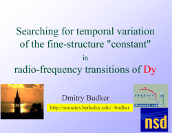
Searching for temporal variation of the fine
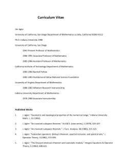
Curriculum Vitae - UCSD Math - University of California San Diego
atlas
DengRenormalization.ppt
pdf
Rare Kaon Decays
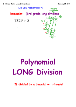
2 - Notes - Polyn Long Division team
[pdf]
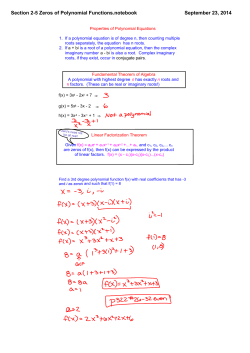
Section 2-5 Zeros of Polynomial Functions.notebook
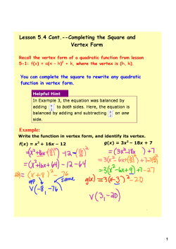
Lesson 5.4 Cont.--Completing the Square and Vertex Form Example:
© Copyright 2026 Paperzz
About Paperzz
DMCA / GDPR
Report
![[pdf]](http://s3.paperzz.com/store/data/007389782_1-e4eaa3b0c1e26281c38f0744e1baba79-250x500.png)