1
Comparison of EKF and UKF for spacecraft
localization via angle measurements
Antonio Giannitrapani Member, IEEE, Nicola Ceccarelli,
Fabrizio Scortecci, Andrea Garulli Senior Member, IEEE
Abstract
In this paper, the performance of two nonlinear estimators is compared for the localization of a
spacecraft. It is assumed that range measurements are not available (like in deep space missions) and
the localization problem is tackled on the basis of angles-only measurements. A dynamic model of the
spacecraft accounting for several perturbing effects, such as Earth and Moon gravitational field asymmetry
and errors associated with the Moon ephemerides, is employed. The measurement process is based on
elevation and azimuth of Moon and Earth with respect to the spacecraft reference system. Position and
velocity of the spacecraft are estimated by using both the Extended Kalman Filter (EKF) and the Unscented
Kalman Filter (UKF). The behavior of the filters is compared on two sample missions: Earth-to-Moon
transfer and geostationary orbit raising.
Index Terms
Spacecraft localization, Nonlinear estimation, Extended Kalman Filter, Unscented Kalman Filter.
I. I NTRODUCTION
Nonlinear estimation techniques play a crucial role in any autonomous navigation system (e.g., see [1],
[2], [3]). It is a fact that many of the problems to be faced in order to achieve full autonomy can be
Antonio Giannitrapani and Andrea Garulli are with the Dipartimento di Ingegneria dell’Informazione, Università di Siena, Siena,
Italy. Email: {giannitrapani,garulli}@dii.unisi.it.
Nicola Ceccarelli, formerly with the Dipartimento di Ingegneria dell’Informazione, Università di Siena, is now with GE Oil &
Gas, Firenze, Italy. Email: [email protected].
Fabrizio
Scortecci
is
with
[email protected].
AEROSPAZIO
Tecnologie
s.r.l.,
Rapolano
Terme,
Siena,
Italy.
Email:
2
cast as estimation problems. Among others, the ability of estimating the position of a spacecraft from the
information provided by its onboard sensors (localization problem) is of paramount importance for the
success of any mission.
This is especially true when dealing with spacecraft propelled by electric propulsion systems (EPS).
Small and cheap electrically propelled spacecraft have recently gained a growing interest for lunar and
outer planetary explorations, after the the successful SMART-1 mission of the European Space Agency [4],
[5]. The use of EPS for the final stint of satellite launching (so called Chemical-Electric missions for Orbit
Raising, C-EOR) is more and more adopted by companies, thanks to their good trade-off between on-orbit
delivery time and propellant required [6]. However, the low thrust produced by a EPS leads to a continuous
thrusting strategy which, in turn, requires an accurate knowledge of the spacecraft position and attitude
during the transfer orbit. Therefore, accurate localization capabilities become a fundamental requirement
for this type of missions.
Localization of spacecraft is usually very accurate when GPS range measurements are available [2]. The
problem becomes more challenging when GPS signals are not available, like in high-Earth orbits or in long
range missions, such as Earth-to-Moon transfers. In these cases, spacecraft navigation is often handled by
ground-based tracking stations, thus making it unfeasible for low-cost spacecraft missions. In order to make
spacecraft fully autonomous, it is necessary to devise self-localization and navigation algorithms relying
only on measurements provided by onboard sensors [3], [7].
In this paper, the problem of spacecraft self-localization is addressed using angular measurements. First,
a dynamic model of the spacecraft is formulated, which takes into account several perturbing effects such
as Earth and Moon gravitational field asymmetry and errors associated with the Moon ephemerides (see
e.g. [8], [9]). It is assumed that the navigation system is able to estimate the spacecraft attitude (by using a
star tracker sensor [10]), and the spacecraft is equipped with line of sight sensors providing measurements
of elevation and azimuth of Moon and Earth with respect to the spacecraft reference system (see e.g. [11],
[12]). Range measurements, which are often difficult to obtain or not sufficiently reliable, are not required.
Then, position and velocity of the spacecraft are estimated by employing both the classical Extended
Kalman Filter (EKF) [13] and the recently developed Unscented Kalman Filter (UKF) [14]. Comparisons
between EKF and UKF have been proposed in several contexts, ranging from target tracking [15], [16], to
3
positioning systems [17], [18] , virtual reality [19]. The filters have been tested on simulated data concerning
two different missions (Earth-to-Moon transfer and GEO orbit raising). The resulting localization errors,
and the associated confidence intervals, show that the proposed algorithms provide reliable estimates, whose
accuracy is sufficient for autonomous navigation in the considered class of missions. Preliminary results
have been presented in [20].
The paper is organized as follows. In Section II the spacecraft dynamic model and the measurement
process are introduced. The localization problem is formulated in Section III, and the adopted nonlinear
estimators are briefly recalled. Section IV reports results from numerical simulations of a Earth-to-Moon
transfer and a geostationary orbit raising. Finally, some conclusions are drawn in Section V.
II. S PACECRAFT MODEL
The following dynamic model for the spacecraft is considered
r̈ = −
ṁ = −
µ
r + µm
ρ3
||T||
,
Isp g
rsm
rm
− 3
3
ρsm
ρm
+
T
m
(1)
(2)
where r = [x, y, z]′ , rm = [xm , ym , zm ]′ are the spacecraft and Moon positions in the Earth Centered
Inertial reference system (ECI [21]), see Figure 1. In equations (1)-(2), µ = 398600.4415 km3 /s2 and
µm = 4902.801 km3 /s2 are the gravitational parameters; ρ = krk, ρm = krm k are the distances of the
spacecraft and the Moon from the earth, respectively; rsm = rm − r is the moon position with respect to
the spacecraft, and ρsm = krsm k. The vector T denotes the thrust provided by the propulsion system, m
is the spacecraft mass, and Isp is the specific impulse [21].
0
1
0
1
Spacecraft
0
1
0
1
111
000
1111
0000
000000000000000000000000
111111111111111111111111
0
1
000
111
000000000000000000000000
111111111111111111111111
11111111111
00000000000
000
111
000000000000000000000000
111111111111111111111111
11111111111
00000000000
rsm
000
111
000000000000000000000000
111111111111111111111111
11111111111
00000000000
000
111
000000000000000000000000
111111111111111111111111
00000000000
11111111111
000000000000000000000000
111111111111111111111111
0
00000000000
11111111111
Moon 1
000000000000000000000000
111111111111111111111111
0
1
00000000000
11111111111
000000000000000000000000
111111111111111111111111
0
1
11111111111
00000000000
000000000000000000000000
111111111111111111111111
000
111
0
1
11111111111
00000000000
000000000000000000000000
111111111111111111111111
000
111
1111
0000
000
111
0
1
11111111111
00000000000
000
111
000
111
00000000000
11111111111
000
111
000
111
00000000000
11111111111
000
111
11111111111
00000000000
r
000
111
00000000000
11111111111
11111111111
00000000000
0
1
00000000000
11111111111
0
1
00000000000
11111111111
1
0
11111111111
00000000000
0
1
00000000000
11111111111
1
0
11111111111
00000000000
0
1
00000000000
11111111111
rm
0
1
00000000000
11111111111
0
1
11111111111
00000000000
Earth
0
1
00000000000
11111111111
0
1
11111111111
00000000000
0
1
00000000000
11111111111
0
1
00000000000
11111111111
1
0
11111111111
00000000000
0
1
00000000000
11111111111
000000
111111
1111111
0000000
1
0
11111111111
00000000000
000000
111111
000000
111111
000000
111111
000000
111111
000000
111111
000000
111111
000000
111111
000000
111111
000000
111111
01
Fig. 1.
The ECI reference system
4
If we define the state vector
X = [x, y, z, ẋ, ẏ, ż, m]′
(3)
containing the spacecraft position and velocity, as well as its mass, model (1)-(2) can be rewritten in vector
form as
Ẋ = f (X, u1 , u2 ),
(4)
where the inputs are the motor thrust and the Moon position,
u1 = T,
u2 = rm .
In order to make a fair and easy-to-implement comparison between EKF and UKF, equation (4) is
discretized with sampling time ∆T (UKF is typically applied to discrete-time systems and its extension to
continuous-time systems is the subject of ongoing research, see [22] for a recent contribution). The Euler
forward discretization of the continuous-time dynamics (4) is given by
X(k+1)∆T = Xk∆T + ∆T f (Xk∆T , u1,k∆T , u2,k∆T ).
(5)
In the following, for ease of notation, we will get rid of the dependence on the sampling time ∆T , and
will denote by qk the value of the quantity q at time k∆T .
In a real-world scenario, there exist several sources of uncertainty affecting the deterministic model (5).
First, at time k∆T inputs are not exactly known. Specifically, it is assumed that the propulsion system
generates a perturbed thrust
u1,k = (1 + ωu,k )T̄k ,
(6)
where T̄ denotes the nominal thrust and ωu,k is a discrete-time white stochastic process. Notice that the
thrust perturbation affects also the fuel mass evolution. Moreover, since also the location of the Moon is
not exactly known, the Moon ephemerides algorithm [8] is used to estimate it. Hence, the knowledge of
the Moon position is affected by the error em,k = [ǫmx ,k , ǫmy ,k , ǫmz ,k ]′ , where each component is a
discrete-time white stochastic process. Therefore, if r̄m is the Moon position provided by the ephemerides,
the actual second input becomes
u2,k = r̄m,k + em,k .
(7)
5
A second source of uncertainty is due to perturbing effects neglected in the nominal model, such as
Earth and Moon gravitational field asymmetry, air drag and sun attraction [23]. According to Cowell’s
formulation, these contributions can be modeled by an additive process disturbance in the right hand side
of (1) (see Sec. 8.4 in [8]). By including the perturbing effects and the input perturbations (6)-(7) into the
nominal model (5), one obtains the perturbed discrete-time dynamic model
Xk+1 = Xk + ∆T (f (Xk , (1 + ωu,k )T̄k , r̄m,k + em,k ) + ck ).
(8)
ck = [0, 0, 0, w̄k′ , 0]′ ,
(9)
where
and w̄k ∈ R3 . If we stack all the uncertainty sources of the dynamic model in a discrete-time disturbance
vector
wk = [w̄k′ , ωu,k , e′m,k ]′ ,
(10)
then the time evolution of the spacecraft dynamics can be written as
Xk+1 = fd (Xk , T̄k , r̄m,k , wk ),
(11)
where T̄k and r̄m,k are known inputs, and the definition of fd (·, ·, ·) follows from equations (1)-(4),(8)-(10).
The spacecraft is equipped with sensors that provide angular measurements of azimuth and elevation of
Moon and Earth, with respect to a local reference system centered at the spacecraft and aligned to ECI, see
Figure 2 (recall that it is assumed that the attitude of the spacecraft is known). Noise-free measurements
at sampling instant k are related to the spacecraft and Moon position by the following equations
θe,k = atan2 (−yk , −xk ) ,
!
−zk
,
φe,k = atan p 2
xk + yk2
(12)
(13)
θm,k = atan2 (ym,k − yk , xm,k − xk ) ,
φm,k = atan
p
zm,k − zk
(xm,k − xk )2 + (ym,k − yk )2
(14)
!
,
(15)
where atan2 (y, x) ∈ (−π, π] is the four-quadrant inverse tangent. Recalling that the Moon position rm,k
corresponds to the input u2,k , the equations above can be summarized as
Ȳk = h̄(Xk , u2,k ),
(16)
6
Earth
Moon
Zs
φe
φm
Ys
θe
Xs
Fig. 2.
θm
Angle measurements in the spacecraft reference system
where Ȳ = [θe φe θm φm ]′ and h̄(·, ·) is defined according to equations (12)-(15) and the definitions of
X in (3). Now, by plugging equation (7) into (16), and taking into account the noise nk affecting nominal
measurements Ȳk , the actual measurement equations become
Yk = h̄(Xk , r̄m,k + em,k ) + nk ,
(17)
nk = [vθe ,k , vφe ,k , vθm ,k , vφm ,k ]′
(18)
where
is a discrete-time white noise modeling measurement errors. If we group all the error source entering in
equation (17) in the noise vector
vk = [n′k , e′m,k ]′ ,
(19)
the measurement equation can be rewritten as
Yk = h(Xk , r̄m,k , vk ),
(20)
where r̄m,k is a known signal (the Moon ephemerides), and the definition of h(·, ·, ·) follows from
equations (12)-(19). Notice that the error on the Moon position estimates, coming from the ephemerides
algorithm, enters both the discrete-time process disturbance wk and the discrete-time measurement noise
vk , see equations (10) and (19).
7
III. S TATE ESTIMATION
The estimation of the spacecraft position and velocity boils down to the state estimation problem for
system (11), based on the observations (20). In this section, we will briefly recall the equations of the
estimators that will be adopted in this work. To this purpose, we will refer to the discrete-time model
Xk+1 = fd (Xk , T̄k , r̄m,k , wk ),
(21)
Yk = h(Xk , r̄m,k , vk ).
where T̄k , and r̄m,k are known signals. In the following, the discrete-time process disturbance wk and
measurement noise vk are assumed to have zero mean.
A. Extended Kalman Filter
Let us denote the covariance matrix of the process disturbance by
Qk = E{wk wk′ }
(22)
Rk = E{vk vk′ }.
(23)
and that of the measurement noise by
Since that the error em affects both the dynamic model and the measurement equation, also the crosscovariance between wk and vk , Sk = E{wk vk′ }, must be considered.
+
Let X̂+
k be the state estimate at time k and let Pk be the estimation error covariance matrix at the same
time. Then, the EKF prediction and correction equations are as follows [13].
Prediction
+
X̂−
k+1 = fd (X̂k , T̄k , r̄m,k , 0)
−
Pk+1
= Fk Pk+ Fk′ + Gk Qk G′k
Correction
−
−
X̂+
k+1 = X̂k+1 + Kk+1 [Yk+1 − h(X̂k+1 , r̄m,k+1 , 0)]
−
+
− Kk+1 Vk+1 Sk′ G′k
= [I − Kk+1 Hk+1 ]Pk+1
Pk+1
−
−
′
′
′
′
Kk+1 = [Pk+1
Hk+1
+ Gk Sk Vk+1
][Hk+1 Pk+1
Hk+1
+ Vk+1 Rk Vk+1
′
′
+ Hk+1 Gk Sk Vk+1
+ Vk+1 Sk′ G′k Hk+1
]−1
8
where the superscript “-” denotes the prediction of the corresponding quantity before the measurement at
time k + 1 is processed, and
∂fd
,
Fk =
∂X X̂+ ,T̄k ,r̄m,k ,0
k
△ ∂h
Hk =
,
∂X X̂− ,r̄m,k ,0
∂fd
Gk =
,
∂w X̂+ ,T̄k ,r̄m,k ,0
k
△ ∂h
Vk =
.
∂v X̂− ,r̄m,k ,0
△
△
k
k
Clearly, if the measurements are available with a frequency lower than the chosen sampling frequency
(e.g., every N ∆T ), then the intermediate state estimates are updated according only to the prediction step
(i.e., N prediction steps are performed between two consecutive correction steps).
B. Unscented Kalman Filter
The UKF is a recursive state estimator based on the Unscented Transform, which is a method to
approximate the mean and covariance of a random variable undergoing a nonlinear transformation [14],
[24]. The underlying idea is to estimate the statistics of the transformed variable from a set of 2n+1 points
(called sigma points), with n being the dimension of the considered random variable. Sigma points are
generated deterministically, on the basis of the (known) covariance matrix of the initial random variable
and depending on the parameters of the filter. Unlike the EKF, the UKF does not require the evaluation of
the Jacobians of the functions fd (·) and h(·), since the gains to be used during the estimation are computed
directly from the sigma points. Hence, the UKF represents a possible alternative to the EKF whenever a
linearized model is not accurate enough or the Jacobian computation becomes too cumbersome (e.g., see
[25] for an application of the UKF to the attitude estimation of a multibody satellite).
In the following the UKF update equations are reported for the dynamic model (21) [24]. Let us define
the augmented state vector Xa = [X′ w′ v′ ]′ ∈ RL . Denote by X̂ak and Pka the state estimate and the
corresponding error covariance matrix
′
′
X̂ak = [(X̂+
k ) 0 0]
Sigma-point generation
+
Pk
a
Pk =
0
0
0
Qk
Sk′
0
Sk
Rk
9
For i = 0, . . . , 2L:
X̂ak
p
= X̂a +
(L + λ)Pka i
k
p
X̂ak −
(L + λ)Pka i−L
χai,k
i=0
i = 1, . . . , L
i = L + 1, . . . , 2L
△
′
v ′ ′
= [(χxi,k )′ (χw
i,k ) (χi,k ) ]
where (P )i denotes the i-th column of matrix P .
Prediction
χxi,k+1|k = fd (χxi,k , T̄k , r̄m,k , χw
i,k , k)
X̂−
k+1 =
−
Pk+1
=
2L
X
i=0
2L
X
(m)
Wi
i = 0, . . . , 2L
χxi,k+1|k
(c)
−
x
′
Wi [χxi,k+1|k − X̂−
k+1 ][χi,k+1|k − X̂k+1 ]
i=0
Y i,k+1|k = h(χxi,k+1|k , r̄m,k+1 , χvi,k )
−
Ŷk+1
=
2L
X
(m)
Wi
i = 0, . . . , 2L
Y i,k+1|k
i=0
Correction
PY Y =
2L
X
(c)
−
−
]′
][Y i,k+1|k − Ŷk+1
Wi [Y i,k+1|k − Ŷk+1
i=0
PXY =
2L
X
(c)
−
′
Wi [χxi,k+1|k − X̂−
k+1 ][Y i,k+1|k − Ŷk+1 ]
i=0
−
−1
−
X̂+
k+1 = X̂k+1 + PXY PY Y (Yk+1 − Ŷk+1 )
+
−
′
Pk+1
= Pk+1
− PXY PY−1
Y PXY
(·)
The weights Wi
are computed as follows
(m)
=
(m)
= Wi
W0
Wi
(c)
λ
L+λ ,
(c)
W0
=
=
1
2(L+λ) ,
λ
L+λ (1
− α2 + β),
i = 1, . . . , 2L
where λ = α2 (L + κ) − L, and α, β and κ are the tuning parameters of the filter.
C. Filter covariances
In this section, the covariances of process disturbance wk and of the measurement noise vk used in
the filters are reported. By recalling the definition (10), under the assumption that w̄k , ωu,k , em,k are
10
uncorrelated stochastic processes, the covariance matrix Qk in (22) is block diagonal
Qk = diag([Qw̄ , σu2 , Sem ])
where Qw̄ , σu2 , Sem , are the covariances of the stochastic processes w̄, ωu , em , respectively.
Recall that the process disturbance w̄ accounts for neglected forces acting on the spacecraft. In order
to model such effects, the covariance Qw̄ is taken as the sum of three terms (which basically means to
assume that the corresponding error sources are independent)
Qw̄ = Qe + Qm + Qt .
where Qe and Qm are due to the Earth and Moon gravitational field asymmetry, while Qt takes into
account other unmodeled effects, like air drag and sun attraction.
Matrix Qe has been estimated by evaluating the difference between the gravitational force predicted
by the nominal model
µ
ρ3 r
and the one yielded by the Earth gravitational model JGM-2 [26]. For each
fixed value of ρ, the sample standard deviation has been computed at 900 different spacecraft positions,
uniformly distributed on a sphere of radius ρ centered at the Earth. This results in an estimated covariance
matrix depending on the distance of the spacecraft to the earth
Qe = diag
2.82 · 1020 2.82 · 1020 7.34 · 1020
,
,
ρ8
ρ8
ρ8
km2
.
s4
The same has been done for the Moon gravitational field asymmetry, by considering the model LP-150
[27]. The standard deviations of the modeled disturbance as a function of ρsm has been estimated, giving
a covariance matrix
Qm =
1018
I3×3
ρ8sm
km2
,
s4
where I3×3 is the identity matrix of order 3. The value of the covariance Qt has been chosen as Qt =
σt2 I3×3 , where σt2 plays the role of a tuning knob in the design of the filters. The variance of the input
perturbation ωu is set to σu2 = 0.012 . Finally, the error covariance of the Moon ephemerides algorithm has
been chosen as Sem = 102 I3×3 km2 [28].
Assuming that the measurement errors nk in (18) are uncorrelated and independent of em,k , vk in (19)
can be modeled as a white stochastic process with block diagonal covariance matrix (23) given by
Rk = diag([σv2 I4×4 , Sem ]),
11
where σv2 depends on the sensor accuracy.
Finally, the cross-covariance between wk and vk is given by
010×4
Sk =
03×4
010×3
.
S em
IV. S IMULATION RESULTS
In this section, the performance of the filters is evaluated by simulating two transfer missions, namely
a Earth-to-Moon transfer and a geostationary orbit raising.
The sampling time used to discretize the dynamic model (4) is ∆T = 15 s and the angular measurements (20) are supposed to be available once per hour. This means that both filters perform a correction step
every 240 prediction steps. The standard deviation σt of the disturbance ωt acts as a tuning parameter of
π
both filters. The standard deviation of the angular measurement errors is supposed to be σv = 0.01 180
rad,
according to the accuracy of several off-the-shelf sensors employed in celestial navigation (see e.g. [3],
[11], [12]).
For each filter both the estimation errors and the corresponding standard deviations are evaluated by
comparing the state estimates to the output of an accurate mission simulator, which explicitly accounts for
a number of perturbing effects. In the simulator, the gravitational field asymmetry of Earth and Moon is
considered through the JGM-2 and LP-150 models, respectively. A point-mass approximation is adopted to
model the Sun attraction on the spacecraft. The “cannonball model” is used to take into account the effect
of the solar radiation pressure. The J71 atmospheric model accounts for air drag. Finally, the resulting
differential equations modeling the spacecraft dynamics, and including all the above orbital perturbations,
are integrated through a fifth-order Runge-Kutta method.
A. Earth-to-Moon transfer mission
In the example of Earth-to-Moon transfer mission considered, the initial orbit has the following parameters: eccentricity e = 0.5, inclination i = 10o , altitude perigee a = 3 · 104 km. The forcing input is a
continuous thrust tangential to the trajectory, with
T=T
ṙ
,
kṙk
(24)
12
x
km
km
200
0
−200
0
10
20
30
60
70
20
30
40
50
60
70
40
50
60
70
40
50
60
70
y
200
0
0
10
20
30
40
50
60
70
0
z
10
20
30
z
50
km
km
10
−200
50
0
−50
0
km
km
50
0
−200
Fig. 3.
40
y
200
x
400
200
0
−200
−400
0
−50
0
10
20
30
40
50
60
70
0
10
20
30
day
day
(a) EKF
(b) UKF
Earth-to-Moon transfer mission: x, y, z estimation errors (thick line) and 99% confidence intervals (thin line).
and T = 0.05 N . Results are reported for 70 days of mission, with the spacecraft reaching a final apogee
altitude of 2.04 · 105 km.
Both filters have been initialized with the same initial estimate and covariance matrix:
X̂+
0 = X(0)
km2
km2
km2
P0+ = diag 1 km2 , 1 km2 , 1 km2 , 10−4 2 , 10−4 2 , 10−4 2 , 10−6 kg 2 ,
s
s
s
where X(0) denotes the true initial state vector (see equation (3)).
For the EKF, the standard deviation of the process disturbance ωt has been tuned to σt = 10−5
km
s2 .
Smaller values of σt resulted in a significant lack of consistency of the filter (estimation errors remarkably
outside the 99% confidence intervals). Figure 3(a) shows the EKF estimation errors for coordinates x, y,
z, and the corresponding 99% confidence intervals. In the first column of Table I the sample standard
deviation of the estimation errors are reported (results are averaged over 10 simulation runs). The overall
average localization error turns out to be 48.82 km.
For the UKF, the following parameters have been used for the generation of the sigma points: α = 10−3 ,
κ = 0, β = 2. The standard deviation of the process disturbance ωt has been tuned to σt = 10−7
km
s2 .
In
Figure 3(b) the x, y, z estimation errors and the 99%, confidence intervals are shown. The second column
of Table I reports the sample standard deviation of the estimation errors, averaged over 10 simulation runs.
The overall average localization error is now 38.00 km, with a reduction of about 20% with respect to
the EKF. Moreover, Figures 3(a)-3(b) show that UKF features better consistency properties (error almost
13
always inside the 99% confidence intervals). Notice that these results have been obtained with a value of
σt smaller than that used by the EKF.
EKF
UKF
x (km)
36.80
31.59
y (km)
42.55
31.57
z (km)
10.81
10.94
ẋ (km/s)
1.33 · 10−3
1.07 · 10−3
ẏ (km/s)
1.51 · 10−3
1.18 · 10−3
ż (km/s)
3.43 · 10−4
4.48 · 10−4
TABLE I
E ARTH - TO -M OON TRANSFER MISSION : SAMPLE STANDARD DEVIATION OF ESTIMATION ERRORS .
Also the relative position of Earth, Moon and spacecraft influences the magnitude of the localization
error. Intuition suggests that larger errors can be expected in those configurations in which the three
bodies are aligned, due to poor geometry for angle measurement. This is confirmed by Figure 4, where
the estimated root mean square localization error (RMSE) is plotted against the alignment angle (i.e., the
angle between the spacecraft and Moon directions, as seen from the Earth). The figure refers to the UKF ,
but a similar phenomenon occurs for EKF. The error peaks are mostly grouped around angles zero (Moon
and Earth aligned on opposite side respect to the spacecraft) and ±π (Moon and Earth aligned on the same
side respect to the spacecraft). Conversely, the smallest values correspond to angles close to ± π2 .
100
90
RMSE (km)
80
70
60
50
40
30
20
−π
Fig. 4.
−π/2
0
π/2
π
Root mean square error of position estimation vs. spacecraft-Earth-Moon alignment
14
x
0
−100
0
−200
0
10
20
30
40
50
60
0
10
20
y
30
40
50
60
40
50
60
40
50
60
y
100
Km
100
Km
x
200
Km
Km
100
0
0
−100
−100
0
10
20
40
50
60
10
20
30
z
0
20
0
−20
−20
0
Fig. 5.
0
Km
Km
30
z
20
10
20
30
40
50
60
0
10
20
30
day
day
(a) EKF
(b) UKF
GEO orbit raising: x, y, z estimation errors (thick line) and 99% confidence intervals (thin line).
B. GEO Transfer
The second mission considered is the final stint of a chemical-electric orbit raising (C-EOR) to geostationary orbit [6], [29] (GEO). The initial orbit is characterized by low eccentricity and inclination, altitude
perigee a = 3·104 km and initial spacecraft mass of 1.5·103 kg. The control strategy is again a continuous
thrust tangential to the trajectory as in (24), with T = 0.05 N . The autonomous navigation algorithm was
tested for a period of 60 days of mission, sufficient to complete the satellite orbit raising to GEO.
The parameters of the filters have been chosen as in the Earth-to-Moon transfer mission, except for
σt . For the EKF algorithm the standard deviation associated with the parameter ωt has been tuned to
σt = 10−4
km
s2 ,
whereas in the UKF algorithm the value σt = 10−6
km
s2
was used. Values of σt smaller
than 10−4 led to inconsistent EKF estimates, with estimation errors significantly outside the 99% confidence
intervals.
In Figure 5(a) EKF simulation results are shown. The estimation errors and the corresponding 99%
confidence intervals for satellite position are plotted. The sample standard deviation of the estimation
errors, averaged over 10 simulation runs, is reported in the first column of Table II. The overall average
position errors resulted to be 40.8 km.
Figure 5(b) and the second column of Table II show the position estimation errors and the sample
standard deviation (averaged over 10 runs) for the UKF algorithm. In this case the overall average position
errors are 36.2 km. As far as the localization error is concerned, the UKF provides a 10% improvement.
It is worth remarking that running the EKF with the tuning parameter σt = 10−6
km
s2
(i.e., the same value
15
EKF
UKF
x (km)
32.02
31.02
y (km)
31.27
30.17
z (km)
5.47
6.16
ẋ (km/s)
3.2 · 10−3
3.7 · 10−3
ẏ (km/s)
3.2 · 10−3
3.7 · 10−3
ż (km/s)
0.9 · 10−3
1.7 · 10−3
TABLE II
GEO ORBIT RAISING : SAMPLE STANDARD DEVIATION OF ESTIMATION ERRORS
used for the UKF) results in a complete lack of filter consistency, and the average estimation error turns
out to increase of one order of magnitude.
From Figure 5 it can be observed that the standard deviation of the x and y estimation errors has two
characteristic frequencies, the faster one being approximately 2 cycles per day. It is worth noticing that
also when the standard deviation is small the estimation error is still within the 3σ bounds, as can be seen
in Figure 6(a), where a magnified view of the localization error during the last 10 days of the GEO orbit
raising mission is shown.
Also in this kind of mission the spacecraft-Earth-Moon alignment greatly influences the estimation error
(see Figure 6(b)). The plot refers to UKF estimate, but a similar behavior is observed also for EKF. The
expected error grows as the satellite, the Earth and the Moon approach a collinear configuration, whereas the
most accurate estimates are expected when the satellite sees Earth and Moon along orthogonal directions.
V. C ONCLUSIONS AND FUTURE WORK
The performance of different nonlinear estimation techniques for the autonomous navigation of spacecraft
in low-cost deep space missions has been analyzed. The spacecraft localization problem has been addressed
via both the Extended Kalman Filter and the Unscented Kalman Filter. The localization procedure is based
only on angular measurements of celestial bodies with respect to the spacecraft reference system, and does
not require range measurements which can be difficult to obtain. The behavior of the filters has been tested
on two sample missions, using an accurate mission simulator accounting for several perturbing effects. The
accuracy of both estimators turned out to be satisfactory, featuring average localization errors which are
16
x
Km
200
0
70
−200
50
65
51
52
53
54
55
56
57
58
59
60
60
Km
0
−100
50
51
52
53
54
55
56
57
58
59
60
z
RMSE (km)
y
100
Km
20
55
50
45
40
0
35
−20
50
51
52
53
54
55
56
57
58
59
60
30
−π
0
−π/2
π/2
π
day
(a)
Fig. 6.
(b)
(a) Magnified view of UKF localization error during GEO orbit raising. (b) Effect of spacecraft-Earth-Moon alignment on
localization error.
reasonably small for the type of missions of interest. Although the filters considered in the paper resulted
in localization errors of the same order of magnitude, the UKF has shown better performance in terms of
average localization accuracy and consistency of the estimates.
There are currently two main research lines aiming at analyzing more in depth the suitability of the
considered filters for autonomous navigation. The first one is the enrichment of the dynamic model, in
order to include also the spacecraft attitude among the quantities to be estimated. The second one concerns
the adoption of more accurate sensor models, taking into account the error in estimating the center of
celestial bodies from images, as well as the adoption of a star-tracker camera for attitude estimation.
R EFERENCES
[1] J. Kim and S. Sukkarieh, “Autonomous airborne navigation in unknown terrain environments,” IEEE Transactions on Aerospace
and Electronic Systems, vol. 40, no. 3, pp. 1031–1045, 2004.
[2] T. Upadhyay, S. Cotterill, and A. W. Deaton, “Autonomous GPS/INS navigation experiment for space transfer vehicle,” IEEE
Transactions on Aerospace and Electronic Systems, vol. 29, no. 3, pp. 772–785, 1993.
[3] D. Tuckness and S. Young, “Autonomous navigation for lunar transfer,” Journal of Spacecraft and Rockets, vol. 32, no. 2, pp.
279–285, March-April 1995.
[4] European Space Agency, “http://www.esa.int/specials/smart-1,” 2003.
[5] D. Milligan, D. Gestal, P. Pardo-Voss, O. Camino, D. Estublier, and C. Koppel, “SMART-1 electric propulsion operational
experience.” in Proceedings of the 29th International Electric Propulsion Conference, Princeton, NJ, November 2005.
[6] D. Oh, S. Kimbrel, and M. Martinez-Sanchez, “End-to-End Optimization of Mixed Chemical-Electric Orbit Raising Missions,”
in 38th AIAA/ASME/SAE/ASEE Joint Propulsion Conference, Indianapolis, Indiana, July 2002.
17
[7] A. C. Long, D. Leung, D. Folta, and C. Gramling, “Autonomous navigation of high-Earth satellites using celestial objects and
doppler measurements,” in AIAA/AAS Astrodynamics Specialist Conference, Denver, CO, August 2000.
[8] A. Vallado, Fundamentals of Astrodynamics and Applications, 2nd ed.
Microcosm Press jointly with Kluwer Academic
Publisher, 2001.
[9] J. Salvail and W. Stuiver, “Solar sailcraft motion in Sun-Earth-Moon space with application to lunar transfer from geosynchronous
orbit,” Acta Astronautica, vol. 35, no. 2-3, pp. 215–229, 1995.
[10] J. L. Crassidis, F. L. Markley, and Y. Cheng, “Survey of nonlinear attitude estimation methods,” Journal of Guidance Control
and Dynamics, vol. 30, no. 1, pp. 12–28, 2007.
[11] F. Tai and P. Noerdlinger, “A low cost autonomous navigation system,” in Guidance and control 1989: Proceedings of the
Annual Rocky Mountain Guidance and Control Conference, 1989, pp. 3–23.
[12] R. Hosken and J. Wertz, “Microcosm autonomous navigation system on-orbit operation,” Advances in the Astronautical Sciences,
vol. 88, pp. 491–491, 1995.
[13] J. Crassidis and J. Junkins, Optimal Estimation of Dynamic Systems, ser. Applied mathematics and nonlinear science series.
Chapman & Hall/CRC, 2004.
[14] S. J. Julier and J. K. Uhlmann, “A new extension of the Kalman filter to nonlinear systems,” in Proceedings of AeroSense: The
11th Int. Symp. on Aerospace/Defence Sensing, Simulation and Controls, 1997, pp. 182–193.
[15] A. Farina, B. Ristic, and D. Benvenuti, “Tracking a ballistic target: comparison of several nonlinear filters,” IEEE Transactions
on Aerospace and Electronic Systems, vol. 38, no. 3, pp. 854–867, 2002.
[16] R. Zhan and J. Wan, “Iterated Unscented Kalman Filter for Passive Target Tracking,” IEEE Transactions on Aerospace and
Electronic Systems, vol. 43, no. 3, pp. 1155–1163, 2007.
[17] M. St-Pierre and D. Gingras, “Comparison between the unscented Kalman filter and the extended Kalman filter for the position
estimation module of an integrated navigation information system,” in 2004 IEEE Intelligent Vehicles Symposium, 2004, pp.
831–835.
[18] Y. Yudan and D. A. Grajner-Brzezinska, “Nonlinear Bayesian filter: Alternative ti the Extended Kalma Filter in the GPS/INS
fusion systems,” in Proceedings of the ION GNSS 18th Internetional Technical Meeting of the Satellite Division, 13-16 September
2005, pp. 1391–1400.
[19] J. LaViola Jr, “A comparison of unscented and extended Kalman filtering for estimating quaternion motion,” in Proceedings of
the 2003 American Control Conference, vol. 3, 2003, pp. 2435– 2440.
[20] N. Ceccarelli, A. Garulli, A. Giannitrapani, M. Leomanni, and F. Scortecci, “Spacecraft localization via angle measurements
for autonomous navigation in deep space.” in Proceedings of the 17th IFAC Symposium on Automatic Control in Aerospace.,
Toulouse, FR, June 2007.
[21] J. R. F. M. D. Griffin, Space Vehicle Design, 2nd ed., ser. AIAA education.
AIAA, 2004.
[22] S. Sarkka, “On Unscented Kalman Filtering for state estimation of continuous-time nonlinear systems,” IEEE Transactions on
Automatic Control, vol. 52, no. 9, pp. 1631–1641, 2007.
[23] D. King-Hele, Satellite Orbits in an Atmosphere: Theory and Applications.
Springer, 1987.
[24] E. Wan and R. van der Merwe, “The Unscented Kalman Filter,” in Kalman Filtering and Neural Networks, S. Haykin, Ed.
Wiley, 2001, ch. 7, pp. 221–280.
18
[25] J. Fisher and S. R. Vadali, “Gyroless attitude control of multibody satellites using an unscented kalman filter,” Journal of
Guidance Control and Dynamics, vol. 31, pp. 245–251, 2008.
[26] European Cooperation for Space Standardization, “Space engineering,” 2200 AG Noordwiijk, THe Netherlands, 2000.
[27] A. Konopliv, S. Asmar, E. Carranza, W. Sjogren, and D. Yuan, “Recent gravity models as a result of the lunar prospector
mission,” Icarus, vol. 150, pp. 1–18, Mar. 2001.
[28] P. Seidelmann, E. Santoro, and K. Pulkkinen, “Systematic differences between planetary observations and ephemerides,” in
Second U. S. Hungary Workshop, ser. Dynamical Astronomy.
Univ. of Texas Press, September 1985, pp. 55–65.
[29] R. Killinger, R. Kukies, M. Surauer, H. Gray, and G. Saccoccia, “Final Report on the ARTEMIS Salvage Mission Using Electric
Propulsion,” in 39th AIAA/ASME/SAE/ASEE Joint Propulsion Conference and Exhibit, Huntsville, Alabama, July 20-23 2003.
Antonio Giannitrapani was born in Salerno, Italy, in 1975. He received the Laurea degree in Computer
Engineering in 2000, and the Ph.D. in Control Systems Engineering in 2004, both from the Università di
Siena. In 2005 he joined the Dipartimento di Ingegneria dell’Informazione of the same University, where
he is currently Assistant Professor of Robotics. His research interests include localization and map building
for mobile robots, collective motion for teams of autonomous agents, nonlinear estimation techniques for
autonomous navigation, mobile haptic interfaces.
Nicola Ceccarelli was born in Pisa, Italy, in 1977. He received both Master (’02) degree and Ph.D. (’06)
degree from the Università di Siena at the Dipartimento di Ingegneria dell’Informazione. His research activity
has dealt with mobile robotics, satellite systems and unmanned aerial vehicles. Form 2006 to 2007 he has
been Visiting Scientist at the Air Force Research Laboratory thanks to an award from the U.S. National
Research Council. He is currently with GE Oil&Gas as Lead Engineer/Technologist. His duties are mainly
focused on simulation and modeling of compressor train systems.
19
Fabrizio Scortecci received a MS in Aerospace Engineering at the Università di Pisa in 1990. Since his
graduation he worked as Researcher and then as a Project Manager in various theoretical and experimental
projects related to electric satellite propulsion, aerothermodynamics and spacecraft systems. During the year
2000 he joined AEROSPAZIO Tecnologie s.r.l. working as Senior Scientist and Manager on programs related
to on-orbit application of electric propulsion.
Andrea Garulli was born in Bologna, Italy, in 1968. He received the Laurea in Electronic Engineering from
the Università di Firenze in 1993, and the Ph.D. in System Engineering from the Università di Bologna in
1997. In 1996 he joined the Dipartimento di Ingegneria dell’Informazione of the Universit di Siena, where
he is currently Professor of Control Systems. He has been member of the Conference Editorial Board of
the IEEE Control Systems Society and Associate Editor of the IEEE Transactions on Automatic Control.
He currently serves as Associate Editor for the Journal of Control Science and Engineering. He is author
of more than 120 technical publications; co-editor of the books “Robustness in Identification and Control”, Springer 1999, and
“Positive Polynomials in Control”, Springer 2005; co-author of the book “Homogeneous Polynomial Forms for Robustness Analysis
of Uncertain Systems”, Springer 2009. His present research interests include system identification, robust estimation and filtering,
robust control, mobile robotics and autonomous navigation.
© Copyright 2026 Paperzz