Regret Minimization for Reserve Prices in Second-Price

Regret Minimization for Reserve Prices
in Second-Price Auctions
Nicolò Cesa-Bianchi
Università degli Studi di Milano
Joint work with:
Claudio Gentile (Varese) and Yishay Mansour (Tel-Aviv)
N. Cesa-Bianchi (UNIMI)
Second-Price Auctions
1 / 21
Real-Time Bidding
From: wifiadexchange.com
N. Cesa-Bianchi (UNIMI)
Second-Price Auctions
2 / 21
Real-Time Bidding
SSP (supply-side platforms): assist the seller (publisher)
e.g., by optimizing the reserve price
DSP (demand-side platforms): assist the buyer (advertiser)
e.g., by optimizing bids
RTB process
1
A user visits the publisher website creating an impression
2
A call for bids is sent to ad exchanges through SSP
3
The ad exchanges query DSP for advertisers’ bids
4
The bids are submitted
5
Winner is selected and winner’s ad displayed
N. Cesa-Bianchi (UNIMI)
Second-Price Auctions
3 / 21
Second-price auctions
Mechanism
[Myerson, 1981]
Highest bid B(1) wins, but the price is reduced to the second
highest bid B(2)
Alice bids $0.80 and Bob bids $0.55. Alice wins and pays $0.55
Theorem: Bidding the true value is a dominant strategy
Assume Alice bids B = v, her true value for the impression
Bid less and lose: Alice bids B < v and loses the auction.
Then B < B(2) < v and she lost a payoff of v − B(2)
Bid more and win: Alice bids B > v and wins the auction.
Then v < B(1) < B and she ends up paying B(1) > v
N. Cesa-Bianchi (UNIMI)
Second-Price Auctions
4 / 21
Reserve price: how much the seller values the item
1
Mechanism
If the highest bid B(1) is
below the reserve price,
then the item is not sold
Otherwise, the winning
bid is reduced to the
maximum between the
second highest bid B(2)
and the reserve price
0.8
0.6
0.4
0.2
0
0
0.2
0.6
0.4
(2)
B
0.8
1
(1)
B
Theorem
Bidding the true value is a dominant strategy even in the presence of a
nonzero reserve price
N. Cesa-Bianchi (UNIMI)
Second-Price Auctions
5 / 21
Additional components
Soft floor
Allows to lower the reserve price by running first-price auctions when
the highest bid is between reserve price and soft floor
Estimated Clear Price (ECP)
An estimate of a bid that is likely to win based on historical win rates
Features available to SSP and/or DSP
location and carrier (if user is mobile)
publisher name
website section
placement (identifies a space where the ad can be shown)
banner identifier
user identifier
ECP
N. Cesa-Bianchi (UNIMI)
Second-Price Auctions
6 / 21
Some actual data
N. Cesa-Bianchi (UNIMI)
Second-Price Auctions
7 / 21
Some actual data
N. Cesa-Bianchi (UNIMI)
Second-Price Auctions
8 / 21
The formal auction model
For each impression:
1
Seller chooses reserve price p
2
Bids B1 , . . . , Bm are drawn (hidden from seller)
3
Bidder with highest bid B(1) wins the auction
4
Revenue R(p, B1 , . . . , Bm ) is revealed to seller
Some uncomfortable assumptions
In each auction, bids are drawn i.i.d. from some unknown
distribution
The bid distribution is the same across multiple auctions
Seller knows number of bidders m (or its distribution)
N. Cesa-Bianchi (UNIMI)
Second-Price Auctions
9 / 21
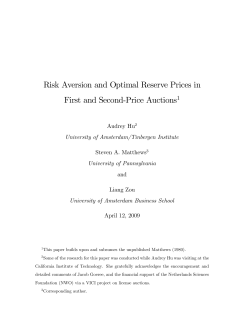
The revenue function
Second-price auction with reserve price
R p, B(1) , B(2) = B(2) I B(2) > p + p I B(2) 6 p 6 B(1)
1
Notation for bids:
B(1) > B(2) > · · ·
Note:
Revenue only depends
on p and two highest
bids B(1) , B(2)
0.8
0.6
0.4
0.2
0
0
0.2
0.4
B(2)
N. Cesa-Bianchi (UNIMI)
Second-Price Auctions
0.6
0.8
1
B(1)
10 / 21
The expected revenue (for a fixed number of bidders)
Z1
h
i
(1)
(2)
µ(p) = E R p, B , B
= P B(2) > x dx + p P B(2) 6 p 6 B(1)
p
1
0.8
0.6
0.4
0.2
0
N. Cesa-Bianchi (UNIMI)
0.2
0.4
0.6
Second-Price Auctions
0.8
1
11 / 21
Remark
If the bid distribution satisfies the monotone hazard rate assumption,
then the optimal reserve price does not depend on number of bidders:
p∗ =
1 − F(p∗ )
f(p∗ )
dF(p)
where F(p) = P B 6 p and f(p) =
dp
We do not assume the monotone hazard rate assumption
N. Cesa-Bianchi (UNIMI)
Second-Price Auctions
12 / 21
Publisher’s regret when using p1 , p2 , . . .
" T
#
X
E
µ(p∗ ) − µ(pt )
p∗ = argmax µ(p∗ )
where
p
t=1
1
0.8
0.6
0.4
0.2
0
0.2
0.6
0.4
pt
N. Cesa-Bianchi (UNIMI)
Second-Price Auctions
0.8
p
1
∗
13 / 21
Control regret in a sequence of T auctions
Since bids are in [0, 1] regret after T auctions is always O(T )
First approach
Partition reserve prices in K = d1/εe bins and pick a reserve price
pk for each bin k
Run a multiarmed bandit algorithm over the set of prices
p1 , . . . , pK
r
T
= O T 2/3
for ε = T −1/3
Regret(T ) 6 |{z}
εT +
ε
approx. | {z }
cost
estim.
cost
This holds without any special assumption on the expected
revenue function
N. Cesa-Bianchi (UNIMI)
Second-Price Auctions
14 / 21
Control regret in a sequence of T auctions
Second approach
Run a stochastic optimization algorithm that computes a sequence
p1 , p2 , . . . of reserve prices to find the maximum of µ
Using pt gives a stochastic revenue Rt such that E[Rt ] = µ(pt )
√ Regret grows like O T only under specific assumptions on µ
(unimodality, smoothness, etc.)
Main question
Can we get T 1/2 regret without any assumption on the expected
revenue function µ?
N. Cesa-Bianchi (UNIMI)
Second-Price Auctions
15 / 21
Main algorithmic idea
Rewrite expected revenue function
Zp
m
(2) + P B(2) 6 x dx − p P B 6 p
µ(p) = E B
|
{z
}
| {z }
0
constant
function of F(p)
m
in terms of F(p) = P B(2) 6 p
Compute approximation of F(·) = P B(2) 6 · by sampling B(2)
Express P B 6 p
Obtain approximation of expected revenue µ
N. Cesa-Bianchi (UNIMI)
Second-Price Auctions
16 / 21
Sampling second prices
Goal: Sample B(2) in order to approximate µ
1
If p = 0, then revenue
is always B(2)
However, E B(2) may
be much smaller than
µ(p∗ )
0.8
Hence, approximating
µ well by setting p = 0
is potentially wasteful
0.2
0.6
0.4
0
0.2
0.4
0.6
0.8
p
N. Cesa-Bianchi (UNIMI)
Second-Price Auctions
1
∗
17 / 21
Approximating the expected revenue
Find a rough
approximation of µ by
using p = 0 a few times
Use this approximation
to find a region of
prices that includes p∗
with high probability
Recurse on this region
using least price as
reserve price
1
0.8
0.6
0.4
0.2
0
0.1
0.3
0.5
0.7
bi
p
1
b∗
p
B(2) is sampled in green region using a nearly optimal reserve price
N. Cesa-Bianchi (UNIMI)
Second-Price Auctions
18 / 21
Controlling regret in each phase
For each phase i = 1, 2, . . . , S
bi
Refine current region using Ti auctions with reserve price p
(least price in current region)
−i
Regret in phase i when phase length is set to Ti = T 1−2
s
√
C
∗
Ti µ(p ) − µ(b
= CT
p i ) 6 Ti
Ti−1
| {z }
confidence interval
from previous phase
Note: Choice of phase length implies that number of phases is
S = 2 log log T
N. Cesa-Bianchi (UNIMI)
Second-Price Auctions
19 / 21
Finishing up
T S X
X
µ(p∗ ) − µ(pt ) 6 µ(p∗ ) − µ(0) T1 +
µ(p∗ ) − µ(b
p i ) Ti
|
{z
} |{z}
√
t=1
61
6
=
T
i=2
S X
√
T+
µ(p∗ ) − µ(b
p i ) Ti
i=2
S
X
√
6 T+
Ti
s
i=2
√
√
6 T + S CT
= O (log log T )
N. Cesa-Bianchi (UNIMI)
C
Ti−1
√ T
Second-Price Auctions
20 / 21
Open problems
Extend to generalized second-price auction
(multiple impressions sold in each auction)
What if number m of bidders is unknown?
What if bidders correlate (using, e.g., ECP)?
N. Cesa-Bianchi (UNIMI)
Second-Price Auctions
21 / 21

Download Report