JRAP 46(2): 186-189. © 2016 MCRSA. All rights reserved.
A Short Empirical Note on State Misery Indexes
Ryan H. Murphy
Southern Methodist University − USA
Abstract: This paper constructs state level Misery Indexes, incorporating recent data on Regional
Pricing Parities. As an application, it draws the Phillips curve derived from a panel of fifty
states plus the District of Columbia in the years 2008-2011. A state level Misery Index will
allow economists and the public to evaluate the overall macroeconomic picture of a regional
economy, just as the Misery Index currently allows in the national and international context.
It is now possible to construct Okun’s Misery Index (Nessen 2008) at the state level using data published by the BEA (see Aten et al., 2012). This note
does so and makes the data available for the period
2008-2011. The Misery Index, defined as the sum of
inflation and unemployment rates, offers a method of
rapidly summarizing macroeconomic conditions.
Both components have been shown to correlate negatively with subjective well-being (Frey and Stutzer,
2002). There is no theoretical reason why it cannot be
applied to states as well as to nations. While intuitions regarding macroeconomic policy center on national governments and central banks, policies of local governments may also be pertinent. Numerous
recent papers have studied “local multipliers,” which
in the Keynesian model should reduce unemployment while increasing inflation (e.g., ChodorowReich et al. 2012; Nakamura and Steinsson, 2014).1 In
addition, state and local policies which shift the aggregate supply curve and include myriad issues
(from labor policy to energy policy) theoretically
should have an impact on local inflation rates.2
State-level data will allow economists and the
public to evaluate whether, for instance, some regions
in the country are enjoying a supply-led boom while
the rest of the United States languishes in minor stagflation. Disaggregating national data more generally
allows broad macroeconomic forces to be interpreted
more clearly in the context of the time and place, with
state-level panel data as an alternative to the national
and international perspectives.
In this note, I find that U.S. states during the Great
Recession exhibited heterogeneity not only in their
unemployment rates but also in the movements of
their price levels. Despite this, the Phillips Curve relation is weak in the panel of states, although it is present and statistically significant. The highest values
for the Misery Index predominantly appear in 2009,
during which inflation resumed (as defined here) but
unemployment rates remained high.
The Bureau of Economic Analysis now publishes
“Regional Price Parities” (RPPs). These can be used
to estimate cost-of-living adjusted incomes by state,
in the same sense that Purchasing Power Parity allows accurate comparisons across countries. 3 These
These are not to be confused with “local multipliers” dependent
on the effects of agglomeration, not aggregate demand (e.g.,
Moretti, 2010). Presumably these local multipliers would also impact at least the unemployment component of the Misery Index,
however.
2 The interpretation of the aggregated “general equilibrium” effects of such policies are often ignored but are policy relevant.
Central banks credibly targeting inflation presumably respond to
policies so as to hit their target in the aggregate, meaning that inflation locally may directly lead to disinflation elsewhere within a
currency area (Murphy, 2015).
3 Note that this is for all fifty states and the District of Columbia.
Regional CPI, which is available at the Bureau of Labor Statistics,
1
State Misery Indexes
187
interstate comparisons, however, can also be used in
conjunction with national data on inflation rates to
construct within-state inflation. This, added to the regional Bureau of Labor Statistics data on state unemployment rates, yields the State Misery Index.
BEA also publishes an “Implicit Regional Price
Deflator” which may be interpreted as a price index.
But the point here is to construct what is analogous to
CPI, so instead national Chain-Weighted CPI was
used as the baseline, with Regional Price Parities
measuring movements around this baseline. Formally, where 𝐶𝑃𝐼𝑡 is the national CPI index value in
year t and 𝑅𝑃𝑃𝑡,𝑖 is the Regional Price Parity in year t
and state i, the State Misery Index is mathematically
defined as,4
𝑆𝑡𝑎𝑡𝑒 𝑀𝑖𝑠𝑒𝑟𝑦 𝐼𝑛𝑑𝑒𝑥𝑡,𝑖 = (
𝐶𝑃𝐼𝑡
𝑅𝑃𝑃𝑡,𝑖
𝐶𝑃𝐼𝑡−1 𝑅𝑃𝑃𝑡−1,𝑖
− 1)
Great Recession approached the Misery Index values
of European countries like Spain or Greece, there are
certain analogues between states in the U.S. and
countries in the Euro Area. As such, Misery Indexes
by state add to the discussion as to whether the
United States is an optimal currency area. It may also
be of use in measuring the “macroeconomic” effects
of state economic development programs, explaining
net in-migration across states (as in Cebula, 2014;
Cebula and Alexander, 2006; c.f. Mulholland and
Hernandez-Julian, 2013), or how it may interact with
economic freedom or subjective well-being more generally (Belasen and Hafer, 2013). While the Misery
Index may most often be cited by wonks and journalists, state level data may still contribute to the scholarly discussion of state policy.
(1)
+𝑢𝑛𝑒𝑚𝑝𝑙𝑜𝑦𝑚𝑒𝑛𝑡 𝑟𝑎𝑡𝑒𝑡,𝑖
Descriptive statistics for the state inflation rates
(the combined CPI and RPP), the state unemployment rates, and the State Misery Indexes can be found
in Table 1. Following this, rankings for the U.S. states
in 2011 are found in Table 2. Finally, a full listing of
the four years of Misery Index data is provided in Table 3.
One small extension to this exercise is to graph the
two components of the misery index against one another, i.e., the Phillips Curve.5 This relationship is
shown in Figure 1. A simple regression finds a negative coefficient, with one percentage point higher inflation corresponding to 0.45 fewer percentage points
in unemployment. However, this regression only explains (unadjusted 𝑅2 ) 8.6% of the variation in unemployment across states and across time. While this
crude test hardly captures all the nuances of aggregate demand, it suggests that both supply-side and
demand-side policies were important in explaining
differences in unemployment rates even during the
Great Recession.
While the Misery Index may be seen as a simple
piece of rhetoric or a questionably weighted construct
(e.g., equally weighting inflation and unemployment
may be incorrect; see di Tella et al., 2001), it offers a
frugal method of evaluating the character of the macroeconomy. Moreover, while no U.S. state during the
is for more general geographic regions of the United States as
well as a select group of Metropolitan Statistical Areas.
4 In practice, for the year 2008, for example, the inflation rate is
taken to be the percent change in CPI from January 2008 to January 2009, while the RPP data is annual. The unemployment rate
is that of December 2008.
Acknowledgements
The author thanks Colin O’Reilly, Daniel Kuehn,
and two anonymous referees for their useful comments and suggestions.
Table 1. Descriptive statistics.
Inflation Rate
mean st.dev.
1.7
1.3
min
-2.1
max
5.0
Unemployment
Rate
8.1
2.0
3.1
13.9
Misery Index
9.7
2.1
4.0
15.2
Note: n=204.
More sophisticated tests of the Phillips Curve at the state level
using nominal wage data have been performed elsewhere. See,
for example, Kumar and Orrenius (2014).
5
188
Murphy
Table 2. States ranked by Misery Index, 2011.
Nebraska
North Dakota
Wyoming
Utah
Iowa
Kansas
Vermont
Oklahoma
Hawaii
Montana
South Dakota
Minnesota
Virginia
Massachusetts
New Hampshire
Missouri
Texas
New Mexico
Maryland
Wisconsin
Idaho
Ohio
Delaware
Louisiana
West Virginia
Florida
Arizona
Arkansas
Colorado
Washington
Pennsylvania
New York
Indiana
Maine
Alaska
Alabama
Connecticut
Kentucky
Tennessee
Mississippi
Georgia
South Carolina
Oregon
Illinois
DC
Michigan
North Carolina
Rhode Island
New Jersey
California
Nevada
Inflation Unemployment Misery Rank
Index
3.2
3.9
7.1
1
4.2
3.1
7.3
2
2.4
5.1
7.5
3
2.8
4.9
7.7
4
2.9
4.9
7.8
5
2.8
5.5
8.3
6
3.7
4.6
8.3
7
3.2
5.2
8.4
8
3.2
5.2
8.4
9
2.9
5.6
8.5
10
4.5
4
8.5
11
3.3
5.3
8.6
12
3.0
5.7
8.7
13
2.0
6.7
8.7
14
3.4
5.5
8.9
15
2.5
6.7
9.2
16
3.0
6.3
9.3
17
2.6
6.8
9.4
18
2.7
6.8
9.5
19
2.8
6.9
9.7
20
3.1
6.6
9.7
21
2.5
7.4
9.9
22
2.8
7.2
10.0
23
3.3
6.8
10.1
24
2.9
7.3
10.2
25
2.5
7.8
10.3
26
2.6
7.7
10.3
27
2.9
7.4
10.3
28
3.2
7.2
10.4
29
3.2
7.4
10.6
30
3.0
7.6
10.6
31
2.8
8
10.8
32
2.4
8.4
10.8
33
3.7
7.2
10.9
34
4.1
6.9
11.0
35
3.4
7.6
11.0
36
2.9
8.1
11.0
37
3.0
8.1
11.1
38
3.3
7.8
11.1
39
2.3
8.9
11.2
40
2.8
8.5
11.3
41
2.9
8.4
11.3
42
3.0
8.5
11.5
43
2.6
9.1
11.7
44
3.1
8.7
11.8
45
2.8
9
11.8
46
3.0
8.8
11.8
47
2.1
9.8
11.9
48
2.9
9
11.9
49
2.4
9.5
11.9
50
1.6
10.3
11.9
51
Table 3. State Misery Index data.
2008
US Average
Alabama
Alaska
Arizona
Arkansas
California
Colorado
Connecticut
Delaware
District of Columbia
Florida
Georgia
Hawaii
Idaho
Illinois
Indiana
Iowa
Kansas
Kentucky
Louisiana
Maine
Maryland
Massachusetts
Michigan
Minnesota
Mississippi
Missouri
Montana
Nebraska
Nevada
New Hampshire
New Jersey
New Mexico
New York
North Carolina
North Dakota
Ohio
Oklahoma
Oregon
Pennsylvania
Rhode Island
South Carolina
South Dakota
Tennessee
Texas
Utah
Vermont
Virginia
Washington
West Virginia
Wisconsin
Wyoming
7.49
12.1
0
8.28
10.6
9
7.94
12.2
0
9.19
8.82
9.37
10.4
6
10.8
9
10.3
7
6.27
9.17
11.7
9
11.3
1
6.59
7.61
10.9
0
7.48
8.39
8.79
8.43
13.8
8
8.40
10.1
0
10.1
0
6.54
5.21
13.0
9
5.74
10.5
2
8.19
8.91
11.5
0
4.07
10.5
3
7.51
11.7
0
8.69
11.2
9
12.6
5
4.03
10.9
1
8.38
8.81
6.49
8.17
10.9
8
9.25
9.17
7.39
2009
12.2
7
12.8
9
8.72
11.1
4
11.4
7
14.9
3
10.9
7
10.7
4
9.49
13.3
3
12.2
5
12.4
3
9.17
9.76
11.8
7
11.3
4
8.41
9.72
12.1
5
10.6
7
8.90
9.49
9.98
13.2
5
8.63
12.6
0
12.1
4
9.23
7.32
15.1
5
7.97
12.4
9
10.6
0
10.9
5
12.2
3
6.67
12.1
1
8.89
12.0
5
10.6
8
12.7
6
12.5
2
8.79
11.5
3
10.1
6
9.13
7.04
8.87
11.2
7
11.7
5
10.2
5
8.46
2010
10.7
3
6.16
10.0
0
10.1
3
6.65
14.5
3
10.6
5
9.18
7.36
14.8
9
10.7
4
9.19
9.11
9.90
11.0
4
9.57
6.52
6.21
9.00
6.97
10.1
8
8.61
9.08
9.98
8.18
8.55
7.70
8.37
4.86
13.5
3
6.64
10.5
3
9.57
10.9
1
10.1
5
5.55
8.09
5.26
11.6
8
9.13
11.9
3
9.90
4.79
8.53
8.01
8.18
7.66
8.33
10.9
3
7.14
9.29
8.42
2011
10.3
9
10.9
6
10.9
5
10.2
7
10.2
9
11.9
3
10.3
9
10.9
9
9.99
11.7
6
10.2
7
11.2
8
8.44
9.71
11.6
8
10.8
4
7.79
8.27
11.1
0
10.1
4
10.9
3
9.50
8.73
11.7
8
8.61
11.1
9
9.24
8.49
7.13
11.9
4
8.87
11.8
9
9.36
10.8
0
11.8
0
7.25
9.94
8.43
11.4
9
10.5
9
11.8
6
11.2
9
8.55
11.1
4
9.29
7.68
8.31
8.69
10.5
9
10.1
9
9.68
7.46
2008-11
Average
10.22
10.53
9.49
10.56
9.09
13.40
10.30
9.93
9.05
12.61
11.04
10.82
8.25
9.63
11.59
10.76
7.33
7.95
10.79
8.81
9.60
9.10
9.06
12.22
8.46
10.61
9.80
8.16
6.13
13.43
7.30
11.36
9.43
10.39
11.42
5.89
10.17
7.52
11.73
9.77
11.96
11.59
6.54
10.53
8.96
8.45
7.37
8.51
10.94
9.58
9.60
7.93
State Misery Indexes
189
Figure 1. Phillips Curve Using Components of Misery Index
6
5
4
Inflation Rate
3
2
1
0
0
2
4
6
8
10
12
14
16
-1
-2
-3
Unemployment Rate
References
Aten, B., E.B. Figueroa, and T.M. Martin. 2012. Regional Price Parities for State and Metropolitan Areas: 2006-2010. Bureau of Economic Analysis.
www.bea.gov/scb/pdf/2012/08%20August/0812_regional_price_parities.pdf.
Belasen, A.R., and R.W. Hafer. 2013. Do changes in
economic freedom affect well-being? Journal of
Regional Analysis & Policy 43(1): 56-64.
Cebula, R. 2014. The impact of economic freedom
and personal freedom on net in-migration in the
U.S.: a state-level empirical analysis, 2000-2010.
Journal of Labor Research 35(1): 88-103.
Cebula, R., and G.M. Alexander. 2006. Determinants
of net interstate migration, 2000-2004. Journal of
Regional Analysis & Policy 36(2): 116-123.
Chodorow-Reich, G., L. Feiveson, Z. Liscow and
W.G. Woolston. 2012. Does state fiscal relief during recessions increase employment? Evidence
from the American Recovery and Reinvestment
Act. American Economic Journal: Economic Policy
4(3): 118-145.
di Tella, R., R.J. MacCollouch, and A.J. Oswald. 2001.
Preferences over inflation and unemployment:
evidence from surveys of happiness. American
Economic Review 91(1): 335-41.
Frey, B.S., and A. Stutzer. 2002. What can economists
learn from happiness research? Journal of Economic Literature 40(2): 402-435.
Kumar, A., and P. Orrenius. 2014. A closer look at
the Phillips Curve using state-level data. Federal
Reserve Bank of Dallas Working Paper no. 1409,
Federal Reserve Bank of Dallas.
Moretti, E. 2010. Local multipliers. American Economic Review: Papers and Proceedings 100: 1-7.
Mulholland, S., and R. Hernandez-Julian. 2013. Does
economic freedom lead to selective migration by
education?” Journal of Regional Analysis & Policy
43(1): 65-87.
Murphy, R.H. 2015. Beggaring thy neighbor at the
state and local level. Working paper, the O’Neil
Center for Global Markets and Freedom, Southern Methodist University. http://papers.ssrn.com/
sol3/papers.cfm?abstract_id=2657788.
Nakamura, E., and J. Steinsson. 2014. Fiscal stimulus
in a monetary union: evidence from U.S. regions.
American Economic Review 104(3): 753-792.
Nessen, R. 2008. The Brooking’s Institution’s Arthur
Okun – father of the ‘Misery Index.’ Washington
D.C.: Brookings Institution. November 18.
www.brookings.edu/research/opinions/2008/12/17-miseryindex-nessen.
© Copyright 2026 Paperzz