課題名: 超幾何微分方程式の計算解析 (基盤研究 B) 課題番号: 15340045. 平成 15 年度—平成 18 年度 研究組織 研究代表者: 高山信毅 (神戸大学) 研究分担者: 大阿久俊則 (東京女子大学) 研究分担者: 齋藤睦 (北海道大学) 研究分担者: 野呂正行 (神戸大学) 研究分担者: 福山克司 (神戸大学) 研究分担者: 増田哲 (京都大学) 研究分担者: 松本圭司 (北海道大学) 本報告書は “基盤研究 B, 超幾何微分方程式の計算解析” に関連して発表し た論文のリストの他, プレプリント等をまとめて, “超幾何微分方程式の計算 解析” を総括するとともに, 今後の発展を展望する資料を目指している. 1 1 概説 A-超幾何関数の満たす方程式系を A-超幾何方程式系とよぶ. 超幾何微分方 程式は多変数の連立線形偏微分方程式系である. この微分方程式系を調べる ことにより, 多変数超幾何関数のさまざまな性質を知ることができる. 20 世紀後半の超幾何関数の研究は, 主に二つの理論つまりサイクルとコサ イクルの理論か D-加群の理論を利用してすすめられてきた. 1990 年代より 超幾何関数を解析する第 3 の方法が出現した. それは超幾何微分方程式を計 算機による “計算” または計算の手法からうまれた理論的方法により具体的 に解析し, さらに超幾何関数の性質を調べる方法である. 本研究では, 超幾何微分方程式系の様々な計算解析問題を考察しかつその 応用をさぐるべく関連分野との共同研究も進めた. 成果は以下のとおり. 1. A-超幾何微分差分方程式, Modified A-超幾何方程式, affine toric variety の上の D-加群等, 元々の A-超幾何系のよい性質を受けつぐ新しい方程 式系を提案した. 2. D-加群の局所的取り扱いのためのアルゴリズムを整備した. 3. 多変数超幾何関数, 積分の数値計算法の基礎を与えた. 4. 多変数超幾何関数の電子公式集を作るための基盤を整備した. 5. 超幾何関数の代数幾何への応用や可積分系への応用をさらに進展させた. また本研究費を用いて集会 “超幾何方程式研究会” を毎年開催し, 超幾何方 程式の幅広い側面を明らかにしていくことに寄与した. 国際的研究集会とし ては “2nd international congress of mathematical software” に主体的に関与 し, 超幾何方程式の研究に必要なさまざまな数学ソフトウエアについての有 益なフィードバックを得た. 現在, 萌芽的状態であるが今後取り組みを開始してみたい研究テーマをあ げる. 1. 変数の数が多い超幾何多項式, 超幾何級数をマルコフ連鎖モンテカルロ 法などの最新の乱数生成方法を活用して数値計算する. 2. D-加群の局所的取り扱いのためのアルゴリズム, とくに O/I · O の計 算. ここで I は D の左イデアル. 3. 特異点解消アルゴリズムと真島の不確定特異点での級数解構成アルゴ リズムの融合. 4. 定義域の実代数幾何と実領域での接続公式. 5. 代数方程式系の超幾何解. 2 2 本報告集収録の資料, 解説, 論文等 本報告集には以下の解説のプレプリント, プレプリント, 資料等を掲載した. Links to projects 以外はまだ未発表のプレプリントである. 1. Links to projects (数学ソフトのリスト). 高山, 野呂 他編 2. ICMS2006 video アーカイブの目次. 3. 超幾何方程式研究会のプログラム. 4. A-超幾何微分差分方程式の解空間の次元公式. 小原功任, 高山信毅 5. 平面 3 次曲線 Hasse 標準形に関する周期. 松本圭司 6. On regular b-functions for D-modules. 大阿久俊則 3 発表文献リスト 1. Katsuyoshi Ohara, Yuichi Sugiki, and Nobuki Takayama, Quadratic Relations for Generalized Hypergeometric Functions p Fp−1 , Funkcialaj Ekvacioj 46 (2003), 213–251. 2. Nobuki Takayama, Generating Kummer Type Formulas for Hypergeometric Functions, Algebra, Geometry, and Mathematica Software, Springer, Edited by Michael Joswig and Nobuki Takayama, 131–145. 3. Francisco Castro-Jimenez and Nobuki Takayama, Singularities of the Hypergeometric System associated with a Monomial Curve. Transaction of the American Mathematica Society, 355 (2003), 3761–3775. 4. Edited by M.Joswig and N.Takayama, Algebra, Geometry and Software Systems Springer, 2003. 5. Yasushi Tamura, Isao Hasegawa, Hiromasa Nakayama, Nobuki Takayama, Shuhei Todo, Design and Implementation of a Digital Formula Book for Generalized Hypergeometric Functions, Proceedings of IAMC 2003 (Electronic proceedings at symbolicnet.org), 2003, http://www.symbolicnet.org/conferences/iamc03/program.html 6. Toshinori Oaku, Yoshinao Shiraki, Nobuki Takayama, Algebraic Algorithms for D-modules and Numerical Analysis, Z.M.Li, W.Sit (editors), Computer Mathematics, Proceedings of the sixth asian symposium, 23–39, World scientific, 2003. 3 7. Michel Granger, Toshinori Oaku, Nobuki Takayama, Tangent cone algorithm for homogenenized differential operators, Journal of Symbolic Computation 39 (2005), 417–431. 8. Nobuki Takayama, An Algorithm for Constructing Cohomological Series Solutions of Holonomic Systems, Journal of Japan Society for Symbolic and Algebraic Computation, 10, No.4, (2003) 2–11. 9. Rouchdi Bahloul and Nobuki Takayama, Local Gröbner fan: polyhedral and computational approach, 2005, math.AG/0412044 10. 高山信毅 (Nobuki Takayama), OpenXM プロジェクトの過去,現在, 未来. 数式処理 (Journal of Japan Society for Symbolic and Algebraic Computation), 12, No. 1 (2005), 51–56. http://www.jssac.org/Editor/Suushiki/V12/v121.html 11. Edited by Nobuki Takayama and Andres Iglesias, Proceedings of ICMS 2006, Lecture Notes in Computer Science (LNCS) 4151, 2006. 12. Rouchdi Bahloul and Nobuki Takayama, Local Grobner Fan, to appear in C.R. Acad.Sci. Paris, Ser. I. 13. Nobuki Takayama, Kan — A system for doing algebraic analysis by computer. Distributed from http://www.openxm.org 14. Saito, Mutsumi; Traves, William N., Finite generations of rings of differential operators of semigroup algebras. Proceedings of the 36th Symposium on Ring Theory and Representation Theory, 26–31, Symp. Ring Theory Represent Theory Organ. Comm., Yamanashi, 2004. 15. Saito, Mutsumi; Traves, William N., Finite generation of rings of differential operators of semigroup algebras. J. Algebra 278 (2004), no. 1, 76–103. 16. 齋藤 睦: 「グレブナー基底の現在」 (日比孝之編)数学書房 (2006) (第 7章 決定方程式系とグレブナー基底) 17. Saito, Mutsumi: Primitive ideals of the ring of differential operators on an affine toric variety, math.RA/0505667 to appear in Tohoku Mathematical Journal. 18. Matsumoto, Keiji, Algebraic relations among some theta functions on the bounded symmetric domain of type Ir,r . Kyushu J. Math. 60 (2006), no. 1, 63–77. 4 19. Matsumoto, Keiji; Terasoma, Tomohide, Theta constants associated to coverings of P 1 branching at eight points. Compos. Math. 140 (2004), no. 5, 1277–1301. 20. Matsumoto, Keiji Automorphic forms on the complex and real balls derived from theta constants. With an appendix by Masaaki Yoshida. Kyushu J. Math. 58 (2004), no. 1, 71–104. 21. Matsumoto, Keiji; Terasoma, Tomohide, Theta constants associated to cubic threefolds. J. Algebraic Geom. 12 (2003), no. 4, 741–775. 22. Granger, Michel; Oaku,Toshinori, Minimal filtered free resolutions for analytic D-modules. J. Pure Appl. Algebra 191 (2004), no. 1-2, 157–180. 23. 大阿久俊則:微分作用素環の斉次化と確定特異点型D加群、日比孝之編 「グレブナー基底の現在」(数学書房、2006)、pp.176–196. 24. Tsuda, Teruhisa; Masuda, Tetsu, q-Painleve VI equation arising from q-UC hierarchy. Comm. Math. Phys. 262 (2006), no. 3, 595–609. 25. Masuda, Tetsu, Special polynomials associated with the Noumi-Yamada (1) system of type A5 . Funkcial. Ekvac. 48 (2005), no. 2, 231–246. 26. Masuda, Tetsu, The anti-self-dual Yang-Mills equation and classical transcendental solutions to the Painleve II and IV equations. J. Phys. A 38 (2005), no. 30, 6741–6757. 27. Kajiwara, K.; Masuda, T.; Noumi, M.; Ohta, Y.; Yamada, Y., Cubic pencils and Painleve Hamiltonians. Funkcial. Ekvac. 48 (2005), no. 1, 147–160. 28. Kajiwara, K.; Masuda, T.; Noumi, M.; Ohta, Y.; Yamada, Y., Construction of hypergeometric solutions to the q-Painleve equations. Int. Math. Res. Not. 2005, no. 24, 1439–1463. 29. Masuda, Tetsu, Classical transcendental solutions of the Painleve equations and their degeneration. Tohoku Math. J. (2) 56 (2004), no. 4, 467–490. 30. Kajiwara, K.; Masuda, T.; Noumi, M.; Ohta, Y.; Yamada, Y., Hypergeometric solutions to the q-Painleve equations. Int. Math. Res. Not. 2004, no. 47, 2497–2521. 5 31. Masuda, Tetsu On a class of algebraic solutions to the Painleve VI equation, its determinant formula and coalescence cascade. Funkcial. Ekvac. 46 (2003), no. 1, 121–171. 32. Kajiwara, Kenji; Masuda, Tetsu; Noumi, Masatoshi; Ohta, Yasuhiro; Yamada, Yasuhiko, 10 E9 solution to the elliptic Painleve equation. J. Phys. A 36 (2003), no. 17, L263–L272. 33. Masuda, Tetsu, On the rational solutions of q-Painleve V equation. Nagoya Math. J. 169 (2003), 119–143. 34. Point configurations, Cremona transformations and the elliptic difference Painlevé equation, K. Kajiwara, T. Masuda, M. Noumi, Y. Ohta and Y. Yamada, to appear in Seminaires et Congres 14, 175-204. 35. Fukuyama, K., Gap series and functions of bounded variation. Acta Math. Hungar. 110 (2006), no. 3, 175–191. 36. Fukuyama, K., A concrete upper bound in the uniform law of the iterated logarithm. Studia Sci. Math. Hungar. 41 (2004), no. 3, 339–346. 37. Fukuyama, K., An asymptotic property of gap series. III. Acta Math. Hungar. 103 (2004), no. 1-2, 97–106. 38. Fukuyama, K.; Petit, B. An asymptotic property of gap series. II. Acta Math. Hungar. 98 (2003), no. 3, 245–258. 39. Noro, M.: An Efficient Implementation for Computing Groebner Bases over Algebraic Number Fields, in Proceedings of ICMS 2006, LNCS4151, Springer (2006), 99-109. 40. Noro, M.: Modular Dynamic Evaluation, in Proceedings of ISSAC 2006, ICM Press (2006), 262-268. 41. Kawano, Y., Kimura, K., Sekigawa, H., Noro, M., Shirayanagi, K., Kitagawa, M., Ozawa. M.: Existence of the exact CNOT on a quantum computer with the exchange interaction, Quantum Information Processing, 4(2) (2005), 65-85. 42. 野呂 正行: Dynamic Evaluation の実装について, 数式処理 vol. 11, No. 3,4 (2005), 21-18. 43. Noro, M. and Yokoyama, K.: Implementation of prime decomposition of polynomial ideals over small finite fields, Journal of Symbolic Computation, 38, (2004) 1227-1246 6 44. Noro, Masayuki; Yokoyama, Kazuhiro Implementation of prime decomposition of polynomial ideals over small finite fields. J. Symbolic Comput. 38 (2004), no. 4, 1227–1246. 7 Links to Projects. Mathematical Software, icms2006—developer’s meeting This document is a collection of links and descriptions of projects related to icms2006—developer’s meeting. 1. ActiveMath http://www.activemath.org License: Free and open-source for public educational institution ActiveMath is a learning environment for mathematics. It is a web-server based on java servlets which presents semantic OMDoc content to contemporary web-browsers with good quality. ActiveMath supports the learning experience by modelling the learners’ competencies in a learner-model that is fed by tracking the reading and the interactive exercises. The interactive exercises can be rich and multiple-steps exercises and use computer-algebra-systems to evaluate a learner’s input. The content items of ActiveMath are annotated with pedagogical and mathematical knowledge which allows the learner to obtain courses prepared on demand on given learning goals. Finally, the semantic OMDoc representation allows copy-and-paste of formulae and search for content items by text, annotations, or formulae. 2. Aldor http://www.aldor.org License: Other (BSD like) Aldor is a computer programming language, like Scheme, Java or C]. 3. Algorithms in real algebraic geometry (interactive book) http://perso.univ-rennes1.fr/marie-francoise.roy/bpr-posted1.html License: GPL, others Algorithms in real algebraic geometry, by S. Basu, R. Pollack and M.-F. Roy, is a preliminary test version of an extension of the first edition published by Springer in 2003. This interactive book is based on texmacs, and live examples can be computed within the book through the SARAG maxima library by F. Caruso. The final version is due to be published by Springer. 4. Arageli http://www.unn.ru/cs/arageli License: Free for academic and noncommercial use Arageli is a C++ library for doing symbolic computations. It contains arbitrary precision integer and rational numbers, vectors, matrices, polynomials, modular arithmetic, algorithms for number factorization, linear and integer programming etc. Creating new mathematical structures from existing ones (also in other libraries) is easy. Arageli is used in Skeleton, Integizer, Prelinea projects. 5. The Atlas of Lie Groups and Representations http://atlas.math.umd.edu/ License: This is a project to make available information about representations of semi-simple Lie groups over real and p-adic fields. The software is in an early stage of development. Given a general connected complex group G, the software will compute among other things: parameters for the irreducible representations of G with regular integral infinitesimal character, KazhdanLusztig polynomials for representations with regular integral infinitesimal character, .... etc. ( Alfred G. Noel, University of Massachusetts Boston) 6. BESSELINT http://www.cs.kuleuven.be/˜nines/software/BESSELINT/ License: BESSELINT is a Matlab program to compute integrals of the form ∫ ∞ k ∏ xm Jνi (ai x)dx 0 7. 8. 9. 10. i=1 with Jνi (x) the Bessel function of the ∑ first kind and (real) order νi . The parameter m is a real number such that i νi + m > −1 and the coefficients ai are strictly positive real numbers. In the near future this will be extended to compute the Laplace transform of a product of Bessel functions with possibly an additional factor of 1 + dx2 in the denominator (where d is a real number). (Joris Van Deun and Ronald Cools, K.U.Leuven) CoCoA4 http://cocoa.dima.unige.it/ License: The executables are free The interactive system CoCoA-4.6 offers facilities for COmputations in COmmutative Algebra: Gröbner bases and related operations on ideals and modules, Hilbert functions, factorization of polynomials, and some exact linear algebra. CoCoA-4.6 is well-suited to teaching with its simple and mathematically natural command language, and an extensive online help facility. It is free and runs on most common platforms. CoCoALib http://cocoa.dima.unige.it/ License: GPL, others The C++ library CoCoALib offers data structures and operations for COmputations in COmmuative Algebra, most particularly Gröbner bases. Ease of use through a clean design is paramount (with some concessions to guarantee good performance). The library comes with full documentation and numerous example programs. A “beta” release is anticipated in late 2006. A server and interactive system are planned. Computer Algebra Animation http://www.math.kobe-u.ac.jp/caa License: GPL An experimental project for algorithm animations and graphical or interactive user interface in computer algebra with Java and OpenXM. Coq http://coq.inria.fr License: LGPL Coq is a proof assistant. 11. DEpthLAUNAY http://www.dma.fi.upm.es/mabellanas/delonedepth/ License: QPL DEpthLAUNAY is a C++ software developed with CGAL (http://www.CGAL.org) that computes the following geometric structures given a finite set of points in the plane: convex hull, convex layers, convex levels, Delaunay triangulation, Delaunay layers, Delaunay levels, and Voronoi diagram. Input points can be randomly generated, introduced interactively or simply aquired from image files. ( Manuel Abellanas, Universidad Politecnica de Madrid) 12. Epsilon http://www-calfor.lip6.fr/˜wang/epsilon License: Free for academic and noncommercial use Epsilon is a library of functions implemented in Maple and Java for polynomial elimination and triangular decomposition with (geometric) applications. It has 8 modules and contains more than 70 functions, with documentation, examples, and Maple worksheets. (Dongming Wang, Beihang University, China and UPMC-CNRS, France) 13. GAP http://www.gap-system.org License: GPL GAP is a system for computational discrete algebra, with particular emphasis on Computational Group Theory. GAP provides a programming language, a library of thousands of functions implementing algebraic algorithms written in the GAP language as well as large data libraries of algebraic objects. 14. GAP package Alnuth http://www.gap-system.org/Packages/alnuth.html License: GPL The Alnuth package provides various methods to compute with number fields which are given by a defining polynomial or by generators. Some of the methods provided in this package are written in GAP code. The other part of the methods is imported from the Computer Algebra System KANT. 15. GCLC/WinGCLC http://www.matf.bg.ac.yu/˜janicic/gclc/ License: Free for academic and noncommercial use GCLC/WinGCLC is a tool for visualizing and teaching geometry (and not only geometry), and for producing mathematical illustrations. It has support for a range of geometrical constructions and transformations, for symbolic expressions, parametric curves, program loops, for automated proving of geometrical conjectures, for exporting figures into LaTeX and bitmap format etc. 16. GEX http://www.mmrc.iss.ac.cn/gex/ License: 17. 18. 19. 20. 21. Geometry Expert (GEX) is a software for dynamic geometric diagram drawing and automated geometry theorem proving and discovering. As a dynamic geometry software, GEX can be used to build dynamic visual models to assist manipulating and teaching various mathematical concepts. As an automated reasoning software, GEX can be used to prove and discover hundreds of non-trivial geometry theorems automatically Geometry Expert (GEX) is a software for dynamic geometric diagram drawing and automated geometry theorem proving and discovering. As a dynamic geometry software, GEX can be used to build dynamic visual models to assist manipulating and teaching various mathematical concepts. As an automated reasoning software, GEX can be used to prove and discover hundreds of non-trivial geometry theorems automatically Gfan http://home.imf.au.dk/ajensen/software/gfan/gfan.html License: Gfan is a command line tool for enumerating the reduced Gröbner bases of a polynomial ideal in n variables. Hereby the Gröbner fan, an n-dimensional polyhedral complex, is computed. The tropical variety is a certain subcomplex which can also be computed by the software. Gfan uses Gmp and Cddlib for exact arithmetic and polyhedral computations, respectively. GiNaC http://www.ginac.de/ License: GPL GiNaC looks like a computer algebra system and a library, but the name GiNac is an iterated and recurseive abbreviation for GiNaC is Not a Computer Algebra System. GloptiPoly http://www.laas.fr/˜henrion/software/gloptipoly License: GPL, requires Matlab Matlab/SeDuMi add-on to build and solve convex LMI relaxations of the (generally non-convex) global optimization problem of minimizing a multivariable polynomial function subject to polynomial inequality, equality or integer constraints. (Didier Henrion and Jean-Bernard Lasserre, LAAS-CNRS, Toulouse, France) GiANT: Graphical Algebraic Number Theory http://giantsystem.sourceforge.net License: GPL GiANT is a graphical interface for working with number fields. GiANT offers interactive diagrams, drag-and-drop functionality, and typeset formulas. GiANT is written in Java, but uses KASH to perform its computations. GMP: GNU Multiple Precision Arithmetic Library http://www.swox.com/gmp License: LGPL GMP is a free library for arbitrary precision arithmetic, operating on signed integers, rational numbers, and floating point numbers. There is no practical limit to the precision except the ones implied by the available memory in the 22. 23. 24. 25. 26. 27. machine GMP runs on. GMP has a rich set of functions, and the functions have a regular interface. HOL Light http://www.cl.cam.ac.uk/users/jrh13/hol-light/index.html License: Custom BSD-like HOL Light is a theorem prover for classical higher-order logic. It is a rationalized re-implementation in Objective CAML (OCaml) of Mike Gordon’s original HOL system. HOL Light generates proofs using very low-level primitive inference steps, but has numerous higher-level automated rules and a good library of pre-proved mathematics. ( John Harrison.) jReality http://www.jreality.de License: jReality is a library that allows for interactive manipulation of scientific data on a wide variety of platforms. It is written in Java. The output media include software only Java rendering, hardware accelerated OpenGL rendering stereo viewing, immersive virtual reality applications like in the PORTAL as well as file formats like PIXAR’s renderman and SVG. jtem - Java Tools for Experimental Mathematics http://www.jtem.de License: GPL jtem is a collection of mostly mathematical tools and algorithms implemented in Java. The libraries include a wide range from complex numbers to theta-functions, basic linear algebra and adaptive ODE solvers. Kan/sm1 http://www.openxm.org License: GPL, LGPL Kan/sm1 is originally developed for a computer algebra system for the ring of differential operators D. It is designed to be a backend system with a postscript-like small language. It is now used for a controller of OpenXM communications behind as well as a system for the D. KASH/KANT http://www.math.tu-berlin.de/˜kant/kash.html License: Other KASH/KANT is a computer algebra system specialized for algebraic number theory and its applications. It offers powerful functions for working with number fields, function fields, and local fields, as well as functions for solving Diophantine equations. The KANT shell KASH provides a programming language and an interactive help system. KENZO http://www-fourier.ujf-grenoble.fr/˜sergerar/Kenzo License: KENZO program is a Common Lisp Object System (CLOS) whose purpose is to compute various invariants in Algebraic Topology Framework (mainly homology groups). It implements and uses numerous algebraic structures as 28. 29. 30. 31. 32. dg-algebras, simplicial groups, morphisms, reductions, chain complexes, etc. It allows to compute homology groups of sophisticated spaces. KENZO package for A-infinity structures: ARAIA and CRAIC http://www.ehu.es/aba/investigation.htm License: The package component we add to KENZO allows us to compute A-infinity(co)algebra structures induced on the small module of a reduction if the big dg-module is a (co)algebra. (Ainhoa Berciano Alcaraz) KETpic http://www.kisarazu.ac.jp/˜masa/math/E.html License: Free for academic and noncomercial use KETpic is a macro package for Maple, which generates TEXsource codes for clear drawings. This supports users to draw every kind of complicated figure easily with the highest accuracy. The current version as well as the latest Maple runs on major OS: Windows, Mac and Linux. One can download the package, various samples, the command reference and a template of TEXsource from the indicated web site. (Masayoshi SEKIGUCHI) KNOPPIX/math http://www.knoppix-math.org License: KNOPPIX/Math is a project to archive free mathematical software and free mathematical documents and provide them on KNOPPIX. libMpIeee http://www.mpieee.ua.ac.be License: libMpIeee is a C++ software library for radix 2n or 10m mixed precision floating-point arithmetic, that is fully compliant with the IEEE 754/854 standards for floating-point arithmetic. This implies, among others, that the basic operations as well as the remainder and square root operations are exactly rounded, involving a relative error of at most 0.5 units in the last place (ULP) for round to nearest and 1 ULP for directed roundings. As required by the IEEE 754/854 standards, libMpIeee also provides denormal numbers, signed zeroes, signed infinities and NaN (Not-a-Number). Moreover, the conversions between decimal and binary are implemented to satisfy the same error bound as the basic operations. The elementary functions are computed with a relative error of at most 1 ULP for round to nearest and 2 ULP for directed roundings. More information on the implementation of these elementary functions can be found in the contribution ”Towards reliable software for the evaluation of a class of special functions” by Annie Cuyt and Stefan Becuwe. Linbox http://www.linalg.org License: LGPL LinBox is a C++ template library for exact, high-performance linear algebra computation. 33. LiveTeXmacs ftp://math.cgu.edu.tw/pub/KNOPPIX License: GPL LiveTeXmacs is a knoppix-based live distribution for mathematical education. Many mathematical software systems (Axiom, Gnuplot, Maxima, Octave, R etc) are integrated in this distribution. In addition to this, it also includes free documentations for calculus, mathematical (2D/3D) visualization and stochastic processes etc, which are made by TeXmacs. Web applications, such as PHP, Python, Apache, SQL and Zope etc, are also supported. Especially, the Web Mathematics Interactive is pre-installed as the web application for Maxima, Gnuplot and more. Pre-installed development environment gives a scalability of the distribution even with very few knowledge about linux. 34. Logiweb http://logiweb.eu/ License: GPL Logiweb is an infrastructure for publication and archival of machine verified mathematics. It allows users to publish definitions, theories, lemmas, proofs, and computer programs. The system allows proofs to reference previously published material across the Internet so that users in different sites may build on top of the work of each other. (Klaus Grue, University of Copenhagen) 35. Macaulay2 http://www.math.uiuc.edu/Macaulay2 License: GPL Macaulay2 is a software system to support researches in algebraic geometry and commutative algebra. 36. Magma http://magma.maths.usyd.edu.au License: Commercial Magma is a large, well-supported software package designed to solve computationally hard problems in algebra, number theory, geometry and combinatorics. It provides a mathematically rigorous environment for computing with algebraic, number-theoretic, combinatoric and geometric objects. 37. Maple http://www.maplesoft.com License: Commercial Maple is a tool for solving mathematical problems and creating interactive technical applications. 38. Mathematica http://www.wolfram.com License: Commercial Mathematica is a system for doing mathematics. The cite also provides http://functions.wolfram.com (a data base for special functions) and http://library.wolfram.com (a collection of notebooks). 39. math-polyglot http://www.math.kobe-u.ac.jp/math-polyglot License: GFL, BSD This project is started for editing icms2006 — developer’s meeting DVD’s. It provides sample codes for mathematical software systems in our DVD’s. Samples are grouped with mathematical problems. This project also provides inputs for testing and checking if the installation is properly done to the knoppix-math. The project will be moved to a MediaWiki of knoppix-math after the icms2006. (Nobuki Takayama, Kobe University) 40. MATLAB http://www.mathworks.com License: Commercial Matlab is a language for technical computing and an interactive environment. 41. Mizar http://www.mizar.org License: Mizar project provides a database for mathematics (7000 definitions, 40000 theorems) as well as the mizar system. 42. MPFR library for multiple precision floating point computation http://www.mpfr.org License: LGPL The MPFR library is a C library for multiple-precision floating-point computations with exact rounding (also called correct rounding). It is based on the GMP multiple-precision library. The main goal of MPFR is to provide a library for multiple-precision floating-point computation which is both efficient and has a well-defined semantics. 43. Multi Parametric Toolbox http://control.ee.ethz.ch/˜mpt/ License: GPL The Multi-Parametric Toolbox (MPT) is a free Matlab toolbox for design, analysis and deployment of optimal controllers for constrained linear, nonlinear and hybrid systems. Efficiency of the code is guaranteed by the extensive library of algorithms from the field of computational geometry and multiparametric optimization. The toolbox offers a broad spectrum of algorithms compiled in a user friendly and accessible format: starting from different performance objectives (linear, quadratic, minimum time) to the handling of systems with persistent additive and polytopic uncertainties. Users can add custom constraints, such as polytopic, contraction, or collision avoidance constraints, or create custom objective functions. Resulting optimal control laws can either be embedded into your applications in a form of a C code, or deployed to target platforms using Real Time Workshop. 44. MuPad http://www.mupad.de License: Commercial 45. 46. 47. 48. 49. 50. MuPad is a mathematical expert system mainly symbolic/algebraic computation and numerical calculations with arbitrary accuracy. MuPAD-Combinat http://mupad-combinat.sourceforge.net License: MuPAD-Combinat is an open-source algebraic combinatorics package for the computer algebra system MuPAD http://www.mupad.de. Its main purpose is to provide an extensible toolbox for computer exploration, and foster code sharing between researchers in this area. The core of the package is integrated in the official library of MuPAD since version 2.5.0. NZMATH http://tnt.math.metro-u.ac.jp/nzmath/ License: BSD NZMATH is a number theory oriented calculation system based on the scripting language Python. It is currently providing the Python library package named nzmath, which contains modules for primality testings, factorization, polynomial, matrix, elliptic curves, etc. ( MATSUI Tetsushi, Tokyo Metropolitan University) Octave http://www.octave.org License: GPL GNU Octave is a high-level language, primarily intended for numerical computations. Oorange http://www.oorange.de License: GPL Oorange is a development environment that was initially designed for experimental mathematics but has become a general Java programming tool. It’s main feature is its interactive programming, also known as rapid prototyping. It also fits into component oriented development. OpenMath http://www.openmath.org License: OpenMath is an emerging standard for representing mathematical objects with their semantics, allowing them to be exchanged between computer programs, stored in databases, or published on the worldwide web. OpenXM http://www.openxm.org License: BSD, GPL, FFL OpenXM is an infrastructure for communications among mathematical software systems. The project has proposed protocols OpenXM RFC 100, 101, 102, 103, 104. The OpenXM package is a collection of software systems supporting OpenXM protocols. The current distribution contains asir, sm1, Macaulay 2, PHCpack, gnuplot, polymake, cdd, ntl, pari, supports for Maple, Mathematica, OpenMath, and some small sized systems. 51. webOrigami http://weborigami.score.cs.tsukuba.ac.jp/webOrigami/jsp/ License: Origami assistant on a web. 52. ORMS http://orms.mfo.de License: The Oberwolfach References on Mathematical Software (ORMS) project is a web-interfaced collection of information and links on mathematical software, see http://orms.mfo.de. It presents carefully selected software, including general purpose software systems, teaching software, and more specialized packages up to specific implementations on particular mathematical research problems. Each software package is presented by a short description of its mathematical features, information on basic properties like license type and distribution media are provided, and links to syntax examples, possible demo versions and manuals are given. The ORMS offers a choice of retrieval functions, for example, searching via browsing through a mathematical classification scheme, a structured key word search, and a full text search in the description of the software systems. The success of this project will rely on the co-operation of experienced users from different areas of mathematical software. We therefore encourage discussion (at [email protected]) and we will be grateful to contributions (at [email protected]). 53. Pari-GP http://pari.math.u-bordeaux.fr License: GPL The PARI system is a package which is capable of doing formal computations on recursive types at high speed. It is primarily aimed at number theorists, but is useful to anyone whose primary need is speed. The functionality of PARI is available through a sophisticated programmable calculator, named GP, which also implements many features of high level languages. 54. PHCpack http://www.math.uic.edu/˜jan/download.html License: GPL, free software PHCpack is a package for Polynomial Homotopy Continuation. Version 1 was archived by ACM TOMS as Algorithm 795. Currently it is a platform for “numerical algebraic geometry” providing algorithms developed jointly with Andrew Sommese and Charles Wampler. Contributions made by Anton Leykin, Yusong Wang, Ailing Zhao, and Yan Zhuang. ( Jan Verschelde, UIC.) 55. PHCmaple http://www.math.uic.edu/˜leykin/PHCmaple License: GPL This Maple package provides a convenient interface to the functions of PHCpack, a collection of numerical algorithms for solving polynomial systems using polynomial homotopy continuation. 56. polymake http://www.math.tu-berlin.de/polymake/ License: GPL polymake is a modular, object-oriented tool for experimental discrete geometry. The main applications are dealing with polytopes and polyhedra, polyhedral surfaces, and finite simplicial complexes. It offers an unified interface to a wide variety of free software packages from the field, especially for visualisation. It can be used interactively as well as driven by perl scripts or C++ programs. (Ewgenij Gawrilow, Technische Universität Berlin, and Michael Joswig, Technische Universität Darmstadt) 57. ProofPower http://www.lemma-one.com/ProofPower/index/index.html License: GPL ProofPower is a tool for specification and proof in Higher-Order Logic (HOL) and in the Z Notation, based on a re-engineering of Mike Gordon’s original HOL system. Like other systems in the LCF tradition, it uses a powerful strongly-typed functional programming language (Standard ML) to ensure logical correctness by reducing all proof steps to primitive inferences rules and to provide a rich and extensible repertoire of automated derived inference rules and decision procedures. Its is used commercially for the verification of safety-critical avionics control systems. Libraries of discrete and continuous mathematics have been and continue to be developed to support these applications and for their intrinsic interest. 58. QaoS - Querying Algebraic Objects System http://www.math.tu-berlin.de/˜kant/database.html License: BSD like QaoS (Querying Algebraic Objects System) is a stand-alone solution for access to the KANT databases of algebraic and transcendental field extensions. QaoS transfers information via the hypertext transport protocol (HTTP). It can be accessed through a web interface and various computer algebra systems (GAP 4, KASH 2.56, KASH 3, Maple, and SAGE). 59. R http://www.r-project.org License: GPL R is a system for statistical computing and graphics. 60. Risa/Asir http://www.math.kobe-u.ac.jp/Asir License: Other(FFL, BSD) Risa/Asir is a computer algebra system. Here is a list of some commands: fctr (factorization), gr, nd gr trace (Groebner basis), primadec (primary ideal decomposition), af (factorization over algebraic numbers), ifplot (plot of implicit functions), ox * (OpenXM communication functions), generic bfct (bfunction). 61. SAGE: Software for Algebra and Geometry Experimentation http://sage.scipy.org/sage License: GPL 62. 63. 64. 65. 66. The Python-based computer algebra system SAGE comes with the systems GAP, PARI, Singular. and provides interfaces KASH/KANT, Gnuplot, Octave, Magma, Mathematica, and Maple. It includes functions for basic algebraic geometry, elliptic curves over the rational numbers, modular forms, linear algebra and Z-modules, and noncommutative algebra. SARAG http://perso.univ-rennes1.fr/marie-francoise.roy/bpr-posted1.html License: GPL SARAG(Some Algorithms in Real Algebraic Geometry) is a software library that implements some algorithms in real algebraic geometry written in the free computer algebra system Maxima. SARAG has two main applications: extending the capabilities of Maxima and being part of the interactive version of the book “Algorithms in Real Algebraic Geometry” by S. Basu, R. Pollack, M.-F. Roy, which can be now freely downloaded. sgpviz http://www.gap-system.org/Packages/sgpviz.html License: The GAP package sgpviz is a package designed to visualize finite semigroups through their D-classes or Cayley graphs, as well as to make friendlier the usage of GAP when dealing with finite semigroups. Singular http://www.singular.uni-kl.de License: GPL, others Singular is a Computer Algebra System for polynomial computations with emphasis on the special needs of commutative algebra, algebraic geometry, and singularity theory. Singular’s main computational objects are ideals and modules over a large variety of rings, including local rings and noncommutative G-algebras (in the subsystem Plural). Large variety of algorithms, including those based on Gröbner and standard bases, have powerful implementations in Singular. Strong Noether Position http://www-calfor.lip6.fr/˜hashemi/Noether License: We introduce the notion of a homogeneous ideal in Strong Noether Position (SNP); a new definition for the notion of generic coordinates for some problems. This definition is simple to check, because one can test it for the initial ideal of the ideal with respect to the degree reverse lexicographic ordering. It is explicit, because we can provide an algorithm to decide whether a monomial ideal is in SNP or not. We propose some methods to compute the Castelnuovo-Mumford regularity of an ideal which one of them is more efficient than that of [Bermejo-Gimenez, 2005]. ( Amir Hashemi) Surface Evolver http://www.susqu.edu/facstaff/b/brakke/evolver/ License: The Surface Evolver is an interactive program for the study of surfaces shaped by surface tension and other energies, and subject to various con- 67. 68. 69. 70. straints. A surface is implemented as a simplicial complex (a union of triangles) and is evolved toward minimal energy by a gradient descent method. The Evolver can handle arbitrary topology. Graphical output is available in several file formats. surfex http://www.surfex.algebraicsurface.net License: Freeware surfex is a tool for interactive high quality real algebraic surface visualization. It is mainly an intuitive interface which combines the strenghts of several visualization tools; at the moment, these include surf, javaview, and convert. One of the main features of surfex is the interactive visualization of families of algebraic varieties: The user can introduce parameters into some implicit equations and then play with these parameters via sliders. E.g., this allows one to visualize deformations of surface singularities. All the pictures can easily be exported, either as an animation which shows the whole deformation process, or as a snapshot of a single variety. The user can specify the quality of the output which can range from very high quality for printed publications to lower quality for websites. We also implemented a library for the computer algebra system Singular, called surfex.lib, which enhances the quality of the visualization of surfex using pre-computation of the singular locus etc. SYNAPS http://www-sop.inria.fr/galaad/logiciels/synaps License: GPL SYNAPS (SYmbolic Numeric APplications) is a C++ library devoted to symbolic and numeric computations. It provides data-structures for the manipulation of basic algebraic objects, such as vectors, matrices (dense, sparse, structured), univariate and multivariate polynomials. It contains solvers for univariate and multivariate polynomials, including generalized normal form or subdivision solvers, tools for the manipulatiion of algebraic numbers, for the construction of resultants, ... TC ftp://tnt.math.metro-u.ac.jp/pub/math-packs/tc/ License: GPL TC (Tiny C) is an interpreter of multi-precision C language suitable for floating-point calculations of several thousands digits which often appear in computational algebraic number theory. Furthermore TC ver.4, which is equipped with PARI library and turned TCP ver.1, provides frequently used PARI library functions by C-like functions which are easy to call from TC. (Takashi Fukuda) TeXmacs http://www.texmacs.org License: GPL GNU TeXmacs is a free wysiwyw editing platform for scientists. 71. Virtual Math Laboratories http://www.jreality.de License: GPL Virtual Math Labs is a collection of educational and scientific java web start applications. The library of mathematical experiments shows topics from varies areas, e.g. dynamical systems, polyhedral surfaces, calculus, and curves and surfaces. About this document This document, edited by Masayuki Noro and Nobuki Takayama, is distributed under the GNU Free Documentation License Version 1.2. June 27, 2006. List of contributors of this document: Ainhoa Berciano Alcaraz, Alfred Gerard Noel, Amir Hashemi, Anders Nedergaard Jensen, Anton Leykin, Bernard Mourrain, Chu-ching Huang, Colin Jones, Dongming Wang, Ewgenij Gawrilow, Fabrizio Caruso, Francois Descouens, Fukuda Takashi, Gert Martin Greuel, Jan Verschelde, Jean B. Lasserre, John Abbott, John Harrison, Joris Van Deun, Klaus Ebbe Grue, MATSUI Tetsushi, Manuel Abellanas, Manuel Delgado, MarieFrancoise Roy, Markus Schmies, Masayoshi SEKIGUCHI, Masayuki Noro, Nobuki Takayama, Oliver Labs, Predrag Janicic, Rob Arthan, Sebastian Pauli, Sergey Lyalin, Stefan Becuwe, Viktor Levandovskyy, Xiaoshan Gao, Xin Li, Paul Libbrecht, ICMS2006--- developer's meeting Video Archives 1/1 ページ - ICMS2006 Video Archives 1. 2. 3. 4. 5. 6. 7. 8. 9. 10. 11. 12. Plenary Lectures Session 0. General, Andres Iglesias and Nobuki Takayama Session 1. New Developments on Computer Algebra Packages, Andres Iglesias, Tetsuo Ida Session 2. Interfacing Computer Algebra and Mathematical Visualization, Konrad Polthier Session 3. Computer Mathematics, Freek Weidijk, advisory organizer: Henk Barendregt Session 4. Software for Algebraic Geometry and Related Topics, Nobuki Takayama, advisory organizer: Gert Martin Greuel Session 5. Number Theoretical Software, Ken Nakamula, Michael Pohst Session 6. Methods in Computational Number Theory, David Sevilla, Jaime Gutierrez Session 7. Free Software for Computer Algebra, Joris Van der Hoeven Session 8. Software for Optimization and Geometric Computation, Komei Fukuda, Michael Joswig Session 9. Methods and software for computing mathematical functions, Amparo Gil, Javier Segura Session 10. Access to Mathematics on the Web, Paul Libbrecht To view streaming video, you need QuickTime player 7 or later Free download of QuickTime player . Note: version 6 will not work. http://www.math.kobe-u.ac.jp/icms2006/icms2006-video/index.html 2007/01/29 超幾何方程式研究会 1/2 ページ 超幾何方程式研究会 【超幾何方程式研究会】 を下記日程で開きます. みなさまのお越しをお待ちしております. 11月4日(木曜日) 11月5日(金曜日) 11月6日(土曜日) 13:30 -- 17:00 : 場所 神戸学生青年センター 9:30 -- 17:00 : 場所 神戸学生青年センター 9:15 -- 12:45 : 場所 神戸大学自然科学研究科 3 号棟 6階 野海プロジェクト内 620 号室 ○ 場所について 神戸学生青年センター は, 阪急六甲駅の北側にあります. 神戸大学より徒歩 10 分です. 神戸大学自然科学研究科 3 号棟 の位置 なお会場の収容能力は最大 25 名程度ですので, 参加される方はまえもって 高山までメール下さい (@math.kobe-u.ac.jp の takayama です). ◯ 時間割 (暫定版) --------------------------------------------------------------11/4 (木曜日) 神戸学生青年センター (http://www.ksyc.jp) 13:30 -- 14:30 : 高山 (神戸) 超幾何方程式の無限遠点での解析と解析的グレブナ扇 14:45 -- 15:45 : 松本 (北海道) 白頭絡み目と Theta 関数 16:00 -- 16:30 : 藤堂秀平 (神戸, D1) genus0 の代数曲線の parametrization アルゴリズムと実装 16:30 -- 17:00 : 中山洋将 (神戸, D1) Mora の割り算アルゴリズムと local-b 関数の計算アルゴリズム -------------------------------------------------------------11/5 (金曜日) 神戸学生青年センター (http://www.ksyc.jp) 9:30 -- 10:30 : Vidunas Raimundas (九州, 研), On computaion of Belyi maps (highly ramifies coverings of the projective line) 10:45 -- 11:45 : 鈴木(神戸, 研) シュレジンガー系の古典解とその退化構造 13:00 -- 14:00 : 岩崎(九州) K3曲面上の複素力学系 (C.T.McMullen の仕事の紹介) 14:15 -- 15:15 : 千葉康生(東京, 研) 分数階の擬微分作用素を用いた双曲型方程式の境界値問題 15:30 -- 16:30 : 原岡 (熊本) TBA ( 高山注: 大学院生もなにか話すかも) 16:45 -: 未定 夕方からは 野海プロジェクト内の部屋も使えるようになると思います. --------------------------------------------------------------------11/6 (土曜日) 神戸大学自然科学研究科 3 号棟 6階 野海プロジェクト内 620 号室 [パスワードないと土曜日は入れません. 高山携帯へ連絡を] 9:15 -- 10:15 : 松井優(東京, D1) http://www.math.kobe-u.ac.jp/~taka/2004/hg2004.html 2007/01/29 超幾何方程式研究会 2/2 ページ Grassmann多様体上の構成可能関数のRadon変換の反転公式について 10:30 -- 11:30 : 三町(東京工業), 共鳴条件下での捻れホモロジー --- 局所有限ホモロジーと有限ホモロジーの比較 11:45 -- 12:45 : 斎藤(北海道), アフィントーリック多様体上の微分作用素環とA-超幾何系 午後は自由. 部屋は使えると思います. $Id: hg2004.html,v 1.3 2004/11/04 00:59:28 taka Exp $ http://www.math.kobe-u.ac.jp/~taka/2004/hg2004.html 2007/01/29 超幾何方程式研究会 1/2 ページ ☆☆☆☆☆☆☆☆☆☆☆☆☆☆☆☆☆☆☆☆☆☆☆☆☆☆☆ ☆ 2006年1月6日 (Fri), 1月7日 (Sat) ☆ ☆ "超幾何方程式研究会" (1/6 は朝 9:00 から) ☆ ☆ 神戸大学 理学部 B314 教室 ☆ ☆☆☆☆☆☆☆☆☆☆☆☆☆☆☆☆☆☆☆☆☆☆☆☆☆☆☆ 本年度の超幾何方程式研究会は超幾何関数, 超幾何方程式, 超幾何積分 やそれに関係ある話題をひろく扱う予定です. 超幾何関連ソフトウエア, ポスタ, ホームページ,模型の展示もあります ----------------------------------------------------------------------◆ 時間割りについて: 一日 8 講演まで. 2+2, 2+2. 神戸大昔の時間割り準拠 9:00--10:30 10:50--12:20 13:30--15:00 15:20--16:50 原則 45 分. ☆☆☆☆☆☆☆☆☆ 1/6 (Fri) 9:00 開始です ☆☆☆☆☆☆☆☆☆☆☆☆☆☆ ◯1.1 松本圭司 (北大) 「ζ関数の周期関係式」 ◯1.2. Raimundas Vidunas (九大) 「Zeilberger's algorithm for non-terminating hypergeometric series.」 ◯1.3. 笹野 祐輔 (神戸大, 研究生) 「Higher order Painlev\'e equations of type A_l^{(1)},B_l^{(1)}, C_l^{(1)} and D_l^{(1)}」 ◯1.4. 加藤 満生 (琉球大) 「$_3F_2$の2,3次又は高次変換とSchwarz map」 ◯1.5 斎藤睦 (北大) 「アフィントーリック多様体上の微分作用素環の理論の A-超幾何系への応用に向けて」 ◯1.6 野呂正行 (神戸大) 「Risa/Asirの非可換代数用新機能---気軽に計算してみませんか?」 ◯1.7 金井政宏 (東京大学, 研究支援員) 「交通流に現れる超幾何関数」 ◆◆◆◆◆◆◆◆ 1/7 (Sat) 9:00 開始です ◆◆◆◆◆◆◆◆ ◯2.1. 金子 譲一 (琉球大) 「Selbergのある極値問題について」 ◯2.2. 上野陽一 (熊本大, 学生) 「Appell F_4のrigidityについて」 ◯2.3. 増田哲 (神戸大) 「Painlev\'e 系の特殊解と行列式」 ◯2.4 上原 崇人(九大院数理学府, 学生) 「Periodic solutions to the sixth Painlev\'e equation and dynamical systems on cubic surfaces」 ◯2.5 福山克司 (神戸大) 「乱数と数値積分」 http://www.math.kobe-u.ac.jp/~taka/2005/hg2006.html 2007/01/29 超幾何方程式研究会 2/2 ページ ◯2.6 中山洋将 (神戸大, 学生) Interactive Computer Algebra System の試み --- Interactive Tangent cone アルゴリズム と Interactive Buchberger アルゴリズム ☆☆☆☆☆☆☆☆ 1/7 (Sat) 15:00 で終了. 長くても 16:00 まで. ☆☆☆☆☆☆ ━━━━━━━━━━━━━━━━━━━━━━━━━━━━━━━━━━━ △△△超幾何関連ソフトウエア, ポスタ, ホームページ,模型の展示もあります△△△ (1) 山口君のラプラシアンの固有関数(Bessel function等)による画像圧縮. (2) 小原君の超幾何微分差分用パッケージ. (3) 中山君の interactive CA. (4) Bahloul-高山-Touda の local tropical variety パッケージ. (5) その他, 交渉中 ━━━━━━━━━━━━━━━━━━━━━━━━━━━━━━━━━━━ ------AD-------------------------------------------------------------------┏━┫ ■ 超幾何早春学校, at 北大 (札幌) ┣━━┓ ┃一流研究者による超幾何関数の集中講義. ┃ ┃大学院生への旅費サポート. ┃ ┗▼ ▼┛ < 詳しくはこちら→ http://coe.math.sci.hokudai.ac.jp/sympo/060306/index.html > ------AD-------------------------------------------------------------------- http://www.math.kobe-u.ac.jp/~taka/2005/hg2006.html 2007/01/29 1/1 ページ 超幾何方程式研究会 2007 (プログラム 2006.12.19 版) 会場: 神戸大学 理学部B棟 314 教室 (3.14 教室 と覚えて下さい) 問い合わせ先: 高山信毅 ([email protected]) ☆ 1月11日(木曜日) 1:20--2:20 ガウス超幾何方程式の双曲シュバルツ写像の燕尾特異点について. 佐々木武 (神戸大学) 2:40--3:40 有限鏡映群をモノドロミー群にもつ3階の微分方程式. 加藤満生 (琉球大学) 4:00--5:00 複素射影直線の3次巡回分岐被覆の周期. 服部良平 (北海道大学 M2) ☆ 1月12日(金曜日) 9:20--10:20 ガルニエ系の相空間の合流. 高野恭一,田原伸彦 (神戸大学) 10:40--11:40 位相的ラドン変換とその応用について 松井優(東京大学), 竹内潔(筑波大学), 1:20--2:20 Connection matrices associated with a Selberg type integral and the Racah polynomials (or q 6三町勝久(東京工業大学) 2:40--3:40 冪が整数でも通用するtwisted (co)homology理論 伊藤公毅(京都大学) 4:00--5:00 非斉次な単独常微分方程式の形式冪級数の空間での可解条件 田島慎一(新潟大学) ☆ 1月13日(土曜日) 9:20--10:20 次元の異なる超幾何級数に関する変換公式 梶原 康史(大阪大学) 10:30--11:30 Affine Schwarz map, 西坂龍哉, 小林亮一, 新里祥司 (九州大学, M) 11:40--12:40 未定 (会場で相談) ---午後は自由 (会場も利用できます) http://www.math.kobe-u.ac.jp/~taka/2007/hg2007.html 2007/01/29 A-超幾何微分差分方程式の 解空間の次元公式 1 小原功任 金沢大学理学部計算科学科 高山信毅 神戸大学理学部数学科 はじめに 行列 A = (aij ) ∈ M (d, n, Z) をひとつとる. 行列 A の列ベクトルたち は Zd を張るものとし, A の列ベクトルには零ベクトルは含まれないと仮 定する. また, 差分作用素 Si : f (si ) 7→ f (si − 1) を考える. 定義 1. 微分差分方程式系 H A à n ! X aij xj ∂j − si • f = 0, j=1 à ∂j − d Y (i = 1, . . . , d) (1.1) (j = 1, . . . , n) (1.2) ! a Si ij •f = 0 i=1 を A-超幾何微分差分方程式と呼ぶ. ここで, 交換関係 Si Sj = Sj Si , x i S j = S j xi , si Sj = Sj si + δij Sj ∂i ∂j = ∂j ∂i , si ∂j = ∂j si , xi ∂j = ∂j xi − δij をもつ, 有理関数係数の微分差分作用素環 D = C(x1 , . . . , xn , s1 , . . . , sd )h∂1 , . . . , ∂n , S1 , . . . , Sd , S1−1 , . . . , Sd−1 i を考え, H A を D の左イデアルとみなす. 定義 2. 微分差分作用素環 D の左イデアル I のランクを次で定義する. rank(I) = dimC(x,s) D/I ただし, D/I を C(x, s) 上のベクトル空間と考える. 定義 3 (正規化体積). 行列 A の列ベクトル ai を Rd の点とみなし, {0} ∪ {ai } の凸包のユークリッド体積を m(A) で表すとき, vol(A) = d!m(A) を行列 A の正規化体積と呼ぶ. 定理 1. 行列 A が生成条件を満たすとき, H A のランクは A の正規化体 積 vol(A) と一致する. 行列 A の i 番目の列ベクトルを ai とし, 次のような定積分を考える. à n ! Z X F (β, x) = exp xi tai t−β−1 dt, t = (t1 , . . . , td ) C i=1 このとき, F (β; x) は「形式的に」A-超幾何微分方程式を満たす. また, F (s; x) は「形式的に」A-超幾何微分差分方程式を満たす. ここで「形式 的に」と書いたのは, サイクル C の取り方が一般的には分かっていない からである. この積分表示を介して, A-超幾何微分方程式と, A-超幾何微 分差分方程式は関連している. A-超幾何微分方程式のランクをはじめてシステマティックに研究したの は, Gel’fand, Zelevinsky, Kapranov である. 我々の定理と全く同じ条件の もとで, 1980 年代の終りに, トーリックイデアル IA が Cohen-Macaulay ならば, A-超幾何微分方程式 HA (β) のランク rank(HA (β)) は A の正規 化体積に等しいことを示した. その後, 多くの人が正規化体積に等しくな る条件を研究した. (詳しくは [10] およびその参考文献, 最近の進展につ いては [5] 参照) 我々の定理の証明は, これらの定理および級数解の一様収束性と斎藤睦 氏の隣接関係式に関する結果を用いている. 我々は定理の形を予想するた めに, 計算代数システム Risa/Asir 上で計算機実験を行った. これらの実 験に用いたプログラムは yang パッケージとして公開されている ([6], [7]). また, [11] の p.32, Algorithm 4.5 より, H A よりトーリックイデアル IA が導出されることにも注意したい. 2 à ! 1 1 1 1 例 1. A = のとき, A-超幾何微分差分方程式のランクは 3 0 1 2 3 であり, さらにグレブナ基底の計算から, F = t (f, S1 • f, S2 • f ) に対し て, 差分パッフィアン S1 F = A1 (x, s)F, S2 F = A2 (x, s)F が具体的に得られる. ここで, A1 (x, s), A2 (x, s) は有理式を要素とする行 列. A1 , A2 は複雑なので, ここには載せられないが, 特に x = (1, 1, 0, 1) では 0 1 0 2((3s1 −s2 )2 −1) 85s1 −31s2 −58 1 −s2 ) A1 = − 3(6s1 −2s2 −3)(3s , 31 31 31 3s1 −s2 3 −2 0 2 0 0 1 3s1 −s2 3 −2 0 A2 = 2 3(3s1 −s2 +1) 31s1 −13s2 31 − 4(3s1 −s2 +2) 4(3s1 −s2 +2) 2(3s1 −s2 +2) となる. 2 定理の証明: 代数的部分 この節では定理 1 の証明の前半部分, つまり rank(H A ) ≤ vol(A) (2.1) の証明を与える. 証明の本質的部分は, 斎藤睦により証明された A-超幾何方程式の contiguity relation の存在定理である [8]. この contiguity relation を復習し よう. 超幾何方程式の contiguity relation は一般に複雑であるが, A-超幾 何方程式系の contiguity relation はパラメータを減らす方向へは単純で ある: Φ(β; x) を HA (β) の解とするとき ∂i • Φ(β; x) は HA (β − ai ) の解 なる関係がなりたつ. 証明は [10, Theorem 4.5.10, p.184] をみよ. さて問題は ∂i の逆作用素 C の存在の証明と導出である. つまり C • Φ(β − ai ; x) は HA (β) の解 3 (2.2) となる C の存在証明と導出方法が問題である. 斎藤睦は A が normal という条件をみたすとき C が存在するための 必要十分条件を与えた [8]. C の問題についての一番一般的な解答は, [10] の p.174 から p.186 に書いてある. 定理 2 ([10, (4.43)]). (D[s] · HA (s) + D[s] · ∂i ) ∩ K[s] 6= φ である. とくに ∂i の mod HA (s) での逆は D(s) において存在する. こ こで D = Chx1 , . . . , xn , ∂1 , . . . , ∂n i, D[s] = D[s1 , . . . , sd ], D(s) は s の有 理式と x の多項式を係数とする微分作用素のなす環. R = C(x1 , . . . , xn )h∂1 , . . . , ∂n i とおく. R は rational function 係数の微 分作用素環である. Adolphson の定理 [1] または [10, (4.3)] より, β をあ る代数方程式系 (P) の零点集合の外にある複素数のベクトルに選ぶと, dimC(x) R/(R · HA (β)) = vol(A) が成立する. さて s と x の rational function を係数とする微分作用素環 R(s) = C(s, x1 , . . . , xn )h∂1 , . . . , ∂n i を考え, dimC(x,s) R(s)/(R(s) · HA (s)) を計算しよう. ここで β1 , . . . , βd は不定元 s1 , . . . , sd に置き換えてある. この次元を計算するには HA (s) のグレブナ基底 G(s) を R(s) で計算す ればよい. R(s) での計算では x, s の有理式は係数扱いなので Buchberger アルゴリズムの過程で x, s の多項式でわったり掛けたりするはずである. 1 たとえば f − c(x,s) `g, ` ∈ D[s] みたいな計算. 計算は有限の繰り返し で終了する. したがって, これらの係数の s を数に置き換えたとき上の c(x, s) などが恒等的に消えないとか, 計算途中で主係数が消えない条件 は, s についての有限個の代数方程式系 (Q) でかける. したがって β が この代数方程式系の解でなければ, グレブナ基底 G(s) の s を β で置き 換えたものは, R での HA (β) のグレブナ基底となる. なぜならば HA (β) のグレブナ基底の導出過程と HA (s) のグレブナ基底 G(s) の導出過程は 全く同じになるからである. なお s が (Q) の解のときは, 掛ける係数が 消えたり, 分母が 0 になったり, さらにはグレブナ基底の係数が消えてし まうかも知れないわけで, グレブナ基底の導出過程は一般的には異なる. 4 代数方程式系 (P) と (Q) の零点集合の外にある点 β を考えるとグレ ブナ基底 G(β) に関する標準単項式の個数は vol(A) のはずである. 上の 考察よりこれはもちろん G(s) に関する標準単項式の個数に等しい. した がって, dimC(x,s) R(s)/R(s) · HA (s) = vol(A) である. 以上の準備のもとに (2.1) を証明しよう. 定理 2 を用いると, ∂i の逆作 用素である contiguity relation Ci が存在する. よって ∂i − S ai , Ci − S −ai 達は H A の元である. (Ci − S −ai = −S −ai Ci · (∂i − S ai ) だから). ここで Q ai は 行列 A の i 番目のベクトルをあらわす. つまり, S ai は dk=1 Skaki , Q S −ai は dk=1 Sk−aki . さて生成条件を用いると, n X pi ai = ek ek は k 番目の単位ベクトル i=1 Q pi ai となる整数 pi 達が存在する. よって Sk = S と書ける. pi > 0 pi pi ai なら ∂i は S に mod H A (s) で同値, pi < 0 なら Ci−pi は S pi ai に mod H A (s) で同値. したがって結局, H A の 順序 S1 , . . . , Sd > S1−1 , . . . , Sd−1 > ∂1 , . . . , ∂n でのグレブナ基底 E(s) は, G(s), C̃k − Sk を含 むとしてよい. ここで C̃k が微分作用素であることに注意すると, E(s) の 標準多項式の集合は G(s) の標準単項式の集合に含まれる. よって (2.1) がいえた. 3 定理の証明: 解析的部分 rank(H A ) ≥ vol(A) (3.1) の証明には解析を使う. Gel’fand-Zelevinski-Kapranov は, 同次な A の場 合に HA (β) の 一次独立な m = vol(A) 個の級数解を regular triangulation で構成する方法を与えた [4]. もちろん β は generic でないと構成できな い. この解を f1 (β; x), . . . , fm (β; x) と書く. 命題 1. この級数は x と β についてある開集合の上で収束する. [4] には証明のスケッチしか書いてないので 4 節および B 節にくわしい 証明を与える. 証明の細部の議論は不確定特異点の場合の議論 (これは [4] ではやっていない) にも必要となる. 5 さてこの命題により f1 (s; x), . . . , fm (s; x) (の解析接続) は超幾何微分差 分方程式 HA の解析的な解であることがわかる. さて rank(H A ) < vol(A) と仮定しよう. このとき前の定理の順序 S1 , . . . , Sd > S1−1 , . . . , Sd−1 > ∂1 , . . . , ∂n において H A のグレブナ基底の標準単項式は微分のみを含み仮定よりそ の個数は vol(A) より真に小さい. つまり H A の 微分差分作用素環にお けるグレブナ基底の標準単項式の集合 T は HA (s) の D(s) におけるブレ ブナ基底の標準単項式の集合 T 0 の真部分集合である. 消えた (減った分 の) 標準単項式を ∂ γ とおく. このとき ∂ γ は標準単項式 {∂ α | α ∈ T } の 一次結合でかける. ここで |T | < vol(A). さてこの一次結合の表示式を X ∂γ ≡ cα ∂ α mod H A α∈T と書こう. ここで cα は x, s の有理式である. f1 (s; x), . . . , fm (s; x) は超 幾何微分差分方程式 H A の解なので, X ∂ γ • fi = cα ∂ α • fi α∈T である. ここで G(s) の標準単項式の集合 {∂ δ | δ ∈ T 0 } (|T 0 | = vol(A)) を考える. f1 (β; x), . . . , fm (β; x) は HA (β) の一次独立解 だったので, T 0 に関する Wronski 行列式 ¯ ¯ ¯ f1 (s; x) · · fm (β; x) ¯ ¯ ¯ ¯∂ δ f (s; x) · · ∂ δ f (β; x)¯ m ¯ 1 ¯ ¯ ¯ · · ¯ ¯ ¯ ¯ ¯ ¯ · · ¯ ¯ ¯ ¯ · · は s に generic な数を代入したとき恒等的に 0 ではない. 一方 T 0 は ∂ γ を含み, X ∂ γ • fi = cα ∂ α • fi α∈T を上の行列式に代入すると, 上の Wronski 行列式は恒等的に 0 となる. こ れは矛盾である. 以上で (3.1) の証明が終了した. A が同次で無い場合も我々が 5 節で構成する収束級数を使うと同様に (3.1) が証明できる. 6 4 A-超幾何級数の収束性 (確定特異点の場合) 命題 1 はつまり, A の正則三角形分割 ∆ があたえられたとき, ∆ の各 単体 τi に対して決まる形式級数解 fτi (s; x) が収束することを主張して いる. この節では行列 A が同次条件を満たすと仮定する. すなわち A が à ! 1 ··· 1 A= ∗ という形を持つとする. さて, τ を {1, 2, . . . , n} の d-単体とする. λ ∈ Cn が任意の j 6∈ τ に対 して λj ∈ Z であるとき, λ は τ に対して admissible であるという. 命題 2. Aλ = s かつ, d-単体 τ に対して admissible な λ をとったとき, (τ, λ) で決まる A-超幾何級数 φτ (λ; x) = X l∈L xλ+l Γ(λ + l + 1) は H A の形式的な解になる. ここで L = Ker(A : Zn → Zd ). Proof. まず, (1.1) を満たすことを示す. Aλ = s および Al = 0 より, Pn Pn j=1 aij λj = sj かつ j=1 aij lj = 0 なので, n X xλ+l xλ+l = aij (λj + lj ) aij xj ∂j • Γ(λ + l + 1) Γ(λ + l + 1) j=1 j=1 n X = sj • xλ+l Γ(λ + l + 1) よって φτ (λ; x) が (1.1) を満たすことは明らか. 次に, (1.2) を満たすことを示す. Aλ = s より, à d ! Y a Si ij • f (λ1 , . . . , λj , . . . , λn ) = f (λ1 , . . . , λj − 1, . . . , λn ) i=1 7 に注意して, à d ! Y a Si ij • i=1 xλ+l = Γ(λ + l + 1) à d Y ! a Si ij i=1 • n Y xkλk +lk Γ(λk + lk + 1) k=1 λ+l (λj + lj )x−1 j x = Γ(λ + l + 1) xλ+l = ∂j • Γ(λ + l + 1) よって φτ (λ; x) が (1.2) を満たすことは明らか. 次に, 行列 A に対し, Ker(A : Qn → Qd ) の基底 (列ベクトル) を並べ たもので, 次のように正規化したものを B と置こう. B= 1 .. . ∈ M (n, n − d, Q) 1 ∗ この列ベクトルを b(1) , . . . , b(n−d) と書くことにする. b(i) の第 j 成分を bij と書く. A の第一行から n X bij = 0 j=1 が成り立つ. P L0 = {(k1 , . . . , kn−d ) ∈ Zn−d | n−d k b(i) ∈ Zn } とすると, L0 は Zn−d Pn−d i=1(i) i の Z-部分加群であり, L = { i=1 ki b | k ∈ L0 } である. つまり L は L0 でパラメトライズできる. 添字を入れ替えても一般性を失わないので, τ = {n − d + 1, . . . , n} と すれば, A-超幾何級数は φτ (λ; x) = X l∈L P n−d (i) X xλ+ i=1 ki b xλ+l = Pn−d (i) Γ(λ + l + 1) k∈L0 Γ(λ + i=1 ki b + 1) となる. B の形から λj + n−d X ki bij + 1 = λj + kj + 1 ∈ Z i=1 8 (j = 1, . . . , n − d) が成り立つ. また, 1/Γ(0) = 1/Γ(−1) = 1/Γ(−2) = · · · = 0 であるので, Pn−d X φτ (λ; x) = (i) xλ+ i=1 ki b Pn−d (i) Γ(λ + i=1 ki b + 1) k∈L0 λj +kj +1∈Z>0 (j=1,...,n−d) となる. さらに kj0 = λj + kj , 0 λ = λ− n−d X (j = 1, . . . , n − d) λi b(i) i=1 λ̂ = (λ1 , . . . , λn−d ) と置くと, n−d X (i) ki b =− i=1 n−d X λi b (i) + i=1 n−d X ki0 b(i) i=1 であるので, Pn−d X φτ (λ; x) = k0 ∈L0 +λ̂ k0 ∈Zn−d ≥0 = x λ0 (i) Pn−d 0 (i) xλ− i=1 λi b · x i=1 ki b P Pn−d 0 (i) (i) + Γ(λ − n−d + 1) i=1 λi b i=1 ki b 0 X (xb(1) )k10 · · · (xb(n−d) )kn−d Pn−d 0 (i) Γ(λ0 + i=1 ki b + 1) 0 0 k ∈L +λ̂ k0 ∈Zn−d ≥0 となる. ここで 0 0 k ∈ L + λ̂ ⇐⇒ n−d X ki0 b(i) ∈ Zn i=1 であるから, Appendix 定理 4 より, この級数は (1) (n−d) |xb |, · · · , |xb |<r (4.1) で絶対収束する. さて r < 1 としてもよいから, (4.1) の log をとると, b(k) · (log |x1 |, . . . , log |xn |) < log |r| < 0 ∀k 9 (4.2) が得られる. 単体 τ と r で決まる集合 C(A, τ, r) を次で定義する. ¯ ( ) ¯ > − log |r|, i ∈ 6 τ, ¯ ψ ∈ Rn ¯ ∃ϕ ∈ Rd , ψi − (ϕ, ai ) ¯ = 0, i ∈ τ, ( C(A, τ, r) = すると, 条件 (4.2) と (− log |x1 |, . . . , − log |xn |) ∈ C(A, τ, r) が同値であ ることが分かる. (証明は [3] section 4.) いま ∆ を A の regular triangulation とすると, \ C(A, τ, r) τ ∈∆ は空でない open set. よって共通の収束領域が存在する. 5 A-超幾何級数の収束性 (不確定特異点の場合) 次に A = (aij )i,1,...,d,j=1,...,n ∈ M (d, n, Z) が同次条件を満たさない場合 を考える. このとき, A の列ベクトルを a1 , . . . , an と表し, 各 ai は零ベク トルでないと仮定してよい. 証明には, IA の同次化の手法を用いる. すなわち行列 A に対して, 同 次条件を満たす新しい行列 1 1 ··· 1 1 a 11 a12 · · · a1n 0 à = ··· 0 ad1 ad2 · · · adn 0 を考える. à の列ベクトルを ãi で表す. 方向ベクトルを w̃ = (1, . . . , 1, 0) ∈ Rn+1 と置こう. Toric variety Ià の small Gröbner fan は polyhedral fan であるので, 次の補題が成り立つ. 補題 1. 任意の ε > 0 に対して, ある ṽ ∈ Rn+1 が存在して, w̃(ε) := w̃+εṽ がある最大次元の Gröbner fan の内部に入るようにできる. 特に ṽn+1 = 0 としてよい. Proof. ṽn+1 = 0. としてよいことを示そう. 10 任意の t と任意の重みベクトル w̃ に対して, ordw̃ (xα1 1 ordw̃+t(1,··· ,1) (xα1 1 αn+1 · · · xn+1 ) αn+1 · · · xn+1 ) = = n+1 X i=1 n+1 X w̃i αi w̃i αi + t i=1 n+1 X αi i=1 であるから, 同次式 f に対して, inw̃ (f ) = inw̃+t(1,··· ,1) (f ) (5.1) である. I を C[x1 , . . . , xn+1 ] の同次イデアル, I の Gröbner fan を Ē(I) と する. Ē(I) はいろんな次元の Rn+1 の closed set の集合であり, polyhedral fan の公理を満たす (see [Ziegler]). さて, C̄ ∈ Ē(I), dim C ≤ n を考える. このとき C̄ 6⊆ {w̃ | w̃n+1 = 0} (5.2) となる. 背理法で示そう. w̃ ∈ C をとると, w̃ = (∗, · · · , ∗, 0) であるから, C = {w̃0 ∈ Rn+1 | inw̃ (I) = inw̃0 (I)} (5.3) である. G を <w̃ についての reduced Gröbner base としよう. G の要素 は同次式. [11] の p.XX より, C = {w̃0 | inw̃0 (g) = inw̃ (g) for all g ∈ G}. さて, (5.1) より, inw̃ (g) = inw̃+t(1,··· ,1) (g) であるから, (5.3) より w̃ + t(1, · · · , 1) ∈ C となるが, t 6= 0 とすると, w̃ + t(1, · · · , 1) 6∈ {w̃ | w̃n+1 = 0} なので矛盾する. したがって, (5.2) より Ē(I) を w̃n+1 = 0 で切ると, 最大次元の cone は n 次元の cone になる. 特に最大次元の cone の内点で w̃n+1 = 0 となる 点が存在する. また [11] p.71, Proposition 8.15 より w̃(ε) は secondary polytope の内 点であるから, w̃(ε) たちは à の同一の regular triangulation ∆ を誘導 する. 前小節と同じように τ ∈ ∆ に対して b(i) を定義する. また, ãn+1 の weight が一番悪いことから, 常に n + 1 ∈ τ であることに注意すると, 11 ã1 , . . . , ãn の添字を適当に入れ替えて, τ = {n − d + 1, . . . , n + 1} として も一般性を失わない. さて [10] Theorem 3.4.2 より à n−d ! X ∀k 0 ∈ L0 ∩ S. w̃(ε) · ki0 b(i) + λ ≥ w̃(ε) · λ i=1 ここで, S は Γ 因子の分母に Z≤0 が現れないような集合である. ε → 0 の極限を考えて, w̃ · n−d X ki0 b(i) ≥ 0 ∀k 0 ∈ L0 ∩ S. i=1 また, 補題 3 より, w̃(ε) ∈ C(Ã, τ ) なので, w̃(ε) · b(i) ≥ 0 同様に ε → 0 の極限を考えて, w̃ · b (i) = n X bij ≥ 0 j=1 P à の形から, n+1 j=1 bij = 0 であるから, bi,n+1 ≤ 0 (∀i) がいえる. 0 0 k1 ≥ −λ1 , . . . , kn−d ≥ −λn−d なので, n−d X ki0 bi,n+1 ≤− i=1 n−d X λi bi,n+1 i=1 である. 右辺が正数であることに注意. よって, Pochhammer symbol を 用いると, Γ(λn+1 − m) = Γ(λn+1 )(−λn+1 + 1; m)−1 (−1)m であるから, ¯Ã ¯ ¯ !¯−1 n−d n−d ¯ ¯ ¯ ¯ X X ¯ ¯ ¯ ¯ 0 0 ki bi,n+1 ¯ ki bi,n+1 + 1)¯ = |Γ(λn+1 + 1)| · ¯ −λn+1 ; − ¯Γ(λn+1 + ¯ ¯ ¯ ¯ i=1 i=1 ¯Ã !¯ n−d ¯−1 ¯ X ¯ ¯ 0 0 λi bi,n+1 ¯ ≤ c |Γ(λn+1 + 1)| · ¯ −λn+1 ; − ¯ ¯ i=1 = c (5.4) と Γ-因子が評価できる. 12 さて, s̃ = (s0 , s1 , . . . , sd ) とし, D̃ = C(s̃, x̃)h∂1 , . . . , ∂n+1 , S0±1 , . . . , Sd±1 i と置こう. H à が D̃ の左イデアルであることに注意する. Ãλ̃ = s̃ を満たす λ̃ = (λ1 , . . . , λn+1 ) ∈ Rn+1 をとり, λ = (λ1 , . . . , λn ) と する. Ã-超幾何方程式の解 φ̃λ̃ (x̃) = Pn−d X k0 ∈L0 ∩S と, 級数 φλ (x) = X k0 ∈L0 ∩S 0 (i) x̃λ+ i=1 ki b Pn−d 0 (i) Γ(λ + i=1 ki b + 1) Qn Qn j=1 P 0 λ+ n−d i=1 ki bij j=1 xj Γ(λj + Pn−d i=1 ki0 bij + 1) を考える. (x̃ = (x1 , . . . , xn+1 ), x = (x1 , . . . , xn ).) 定義 4. φλ (x) を φ̃λ (x̃) の dehomonization とよぶ. 命題 3. dehomogenize した級数 φλ (x) は超幾何微分差分方程式を満たし, HA (β) の収束解として一次独立である. Proof. まず, Aλ = s となることから, 超幾何微分差分方程式 H A の形式 解となることは明らかである. 次に一次独立であることを示そう. weight vector w̃(ε) = (1, . . . , 1, 0) + εv ∈ Rn+1 は (1, . . . , 1, 0) ∈ Rn+1 の近傍にあって, Ià のグレブナファンの最大次元錐の内点に入っている ものとする. [10] p.119 より, in(1,...,1,0) Ià の最小生成元は ∂n+1 を含まない. よって, inw̃(ε) Ià = inv (in(1,...,1,0) Ià ) は ∂n+1 を含まないので, M = hinw̃(ε) Ià i = hinw(ε) IA i in C[∂1 , . . . , ∂n+1 ]. ここで, w̃(ε) = (w(ε), 0) で w(ε) を決めた. 実際, {∂ u − ∂ v } を Ià のグレ ブナ基底とすると, ∂ u − ∂ v ∈ Ià =⇒ (∂ u − ∂ v )|∂n+1 =1 ∈ Ià , なので OK. 13 ∂ u |∂n+1 =1 = ∂ u さて, θ̃ = (θ1 , . . . , θn+1 ) とすると, [10] Theorem 3.1.3 より generic な β̃ = (β0 , β), β ∈ Cd に対して, in(−w̃(ε),w̃(ε)) Hà (β̃) は inw̃(ε) Ià と Ãθ̃ − β̃ で生成される. M の standard pairs を T (M ) で表す. [10] Theorem 3.2.10 より hinw̃(ε) Ià , Ãθ̃ − β̃i (5.5) は次の形の #T (M ) = vol(Ã) 個の 1 次独立解を持つ. {x̃λ̃ | (∂ a , T ) ∈ T (M )} ここで, λ̃ は, λ̃i = ai ∈ Z≥0 , i 6∈ T and Ãλ̃ = β̃ で定める. なお, この λ̃ は d-単体 τ に対して admissible である. さて, hinw̃(ε) Ià i = hinw(ε) IA i なので, 方程式系 hinw(ε) IA , Aθ − βi (5.6) と (5.5) の違いは θ1 + · · · + θn + θn+1 − β0 のみであって, 他の方程式は xn+1 , ∂n+1 を含まない. また, 任意の (∂ a , T ) ∈ T (M ) に対して, n + 1 ∈ τ である. よって, (5.6) と (5.5) の解空間は, 対応 xλ 7→ x̃λ̃ (5.7) で同型である. ここで, λ̃ = (λ, λn+1 ), λn+1 は n X λi + λn+1 − β0 = 0 i=1 と定義する. [10] Theorem 2.3.11 および Theorem 3.2.10 より, {x̃λ̃ | (∂ a , T ) ∈ T (M )} 14 は C 上 1 次独立なので, 同型 (5.7) から, vol(A) 個の集合 {xλ | (∂ a , T ) ∈ T (M )} も C 上 1 次独立となる. よって, ½ ¾ xλ a | (∂ , T ) ∈ T (M ) Γ(λ + 1) を初項とする級数解たちは, C 上 1 次独立となる. 最後に収束することを示す. φ̃λ (x̃) は (− log |x1 |, . . . , − log |xn+1 |) ∈ C(Ã, τ, r) で収束する. (r < 1) (5.4) より ¯ ¯ ¯ ¯ ¯ ¯ ¯ ¯ 1 1 ¯ ¯ ¯ ¯ ≤ c ¯ ¯ ¯ Qn ¯ P Pn−d 0 (i) 0 ¯ ¯ ¯ j=1 Γ(λj + n−d ¯ k b + 1) Γ(λ + k b + 1) ij i=1 i i=1 i である. xn+1 = 1 と置くと, − log |xn+1 | = 0 だから w̃(ε) ∈ {y | yn+1 = 0} であ ることを用いて \ C(Ã, τ, r) ∩ {y | yn+1 = 0} τ ∈∆ は Rn の, 空でない open subset である. よって φτ (λ; x) は収束する. 結局, まとめると 補題 2. w̃ = (1, · · · , 1, 0) の近傍の generic な重みベクトル w̃0 に対して w̃0 方向の vol(A) 個の (微分方程式の解とみて一次独立な) H à の超幾何 級数解を構成できる. この級数解の dehomogenization は収束し, H A の 解となる. この方法は非同次な A に対して vol(A) 個の収束解を構成するアルゴ リズムを与えていることにも注意しておく. 6 例 ! à 1 1 1 1 とおく. 例 2. A = 1 2 3 および à = 1 2 3 0 ³ ´ 15 行列 à は同次である. つまり Ià は同次イデアルである. Weight ベク 1 (1, 0, 0, 0) に対して initial ideal inw̃(ε) (Ià ) は トル w̃(ε) = (1, 1, 1, 0) + 100 2 3 ∂1 , ∂1 ∂2 , ∂1 ∂3 , ∂2 で生成される. initial ideal が ∂4 を含まないことに注意 しておこう , [10, Chapter 3] に従い, まず Initial ³ . 級数解を構成するために ´ ¢ ¡ system Ãθ̃ − s̃ • g = 0, inw̃(ε) (Ià ) • g = 0 を解こう. inw̃(ε) (Ià ) に対 する standard pairs (∂ a , T ) は (∂10 ∂21 , {3, 4}), (∂10 ∂20 , {3, 4}), (∂10 ∂22 , {3, 4}) となる. したがって initial system の解空間の基底は (s −2)/3 s0 −1−(s1 −2)/3 x4 , 0 0 s1 /3 a0 −s1 /3 , x1 x2 x3 x4 0 2 (s1 −4)/3 s0 −2−(s1 −4)/3 x4 x1 x2 x3 x01 x12 x3 1 となる ([10]). よって同次化した A-超幾何微分差分方程式 H à は次のよ うな級数解をもつ. µ φ̃1 (λ̃, x̃) = xs40 x2 x4 ¶µ x3 x4 k1 ≥0, k2 ≥−1 (k1 ,k2 )∈L0 µ xs40 x3 x4 µ · x2 x4 ´ k1 ³ ´ k2 −2/3 −1/3 x2 x3 x4 ¶ s31 ³ k1 ≥0, k2 ≥0 (k1 ,k2 )∈L0 xs40 −1/3 −2/3 x1 x3 x4 1 −k2 +2 2 +1 )Γ( 3s0 −s1 −2k ) k1 !(k2 + 1)!Γ( s1 −k1 −2k 3 3 X · φ̃3 (λ̃, x̃) = ³ X · φ̃2 (λ̃, x̃) = ¶ s13−2 k1 ≥0, k2 ≥−2 (k1 ,k2 )∈L0 ´ k1 ³ −2/3 −1/3 x2 x3 x4 ´ k2 2 +3 1 −k2 +3 k1 !k2 !Γ( s1 −k1 −2k )Γ( 3s0 −s1 −2k ) 3 3 ¶2 µ X −1/3 −2/3 x1 x3 x4 x3 x4 ¶ s13−4 ´k2 ´ k1 ³ ³ −2/3 −1/3 −1/3 −2/3 x2 x3 x4 x1 x3 x4 2 −1 1 −k2 +1 k1 !(k2 + 2)!Γ( s1 −k1 −2k )Γ( 3s0 −s1 −2k ) 3 3 ここで L0 = {(k1 , k2 ) | k1 ≡ 0 mod 3, k2 ≡ 0 mod 3}∪{(k1 , k2 ) | k1 ≡ 1 mod 3, k2 ≡ 1 mod 3}. 16 さて, この級数解を dehomogenize することにより A-超幾何微分差分方 程式系 H A の次の収束解を得る. ³ ´ k1 ³ ´ k2 −2/3 −1/3 x1 x3 x2 x3 s1 −2 X φ1 (λ, x) = x2 x3 3 2 +1 k !(k2 + 1)!Γ( s1 −k1 −2k ) 3 k ≥0, k ≥−1 1 1 2 (k1 ,k2 )∈L0 ³ φ2 (λ, x) = x3 s1 −4 3 ´k1 ³ −2/3 x2 x3 ´k2 2 +3 k1 !k2 !Γ( s1 −k1 −2k ) 3 k1 ≥0, k2 ≥0 (k1 ,k2 )∈L0 φ3 (λ, x) = x22 x3 −1/3 x1 x3 X s1 3 ³ X k1 ≥0, k2 ≥−2 (k1 ,k2 )∈L0 −1/3 x1 x3 ´ k1 ³ −2/3 x2 x3 ´ k2 2 −1 k1 !(k2 + 2)!Γ( s1 −k1 −2k ) 3 ここで φk (x) は φ̃k (x) の dehomonization である. 最後に A に対応する超幾何微分差分方程式系を差分方程式に変換した ものの Pfaffian system を掲載しておく. これの導出は H A の Gröbner 基底を用いておこなった. 0 0 1 f f 3x1 x3 −4x22 2(s1 −1)x2 +x21 1 x1 S1 x3 ∂3 • f = − s6x x3 ∂3 • f . 6x2 x3 6x2 2 s1 x1 S1 • f S1 • f − 2x3 − 2x 2x 2 A 2 2 ノート: 定義 2 に関する問題提起 差分方程式におけるランクと解空間の次元とは必ずしも一致しない. 例 としてガンマ関数を考える. Γ(s + 1) = sΓ(s) であるから, S : f (s) 7→ f (s − 1) として, D = C(s)hS, S −1 i のイデアル I = hS −1 − si を考えていることになる. すると, 1 − (s − 1)S ∈ I より, C(s) 上のベクトル空間として D/I ' C(s) であるから, I のランクは rank(I) = dimC(s) D/I = 1. しかし, I の解としてはガンマ関数以外にも, sin(2πks)Γ(s) (k ∈ Z) が存在する. sin(2πks) は pseudoconstant と呼ばれる. 17 B 収束性の証明 命題 1 はつまり, A の正則三角形分割 ∆ があたえられたとき, ∆ の各 単体 τi に対して決まる形式級数解 fτi (s; x) が収束することを主張して いる. B.1 準備 まず, Γ-因子の評価に関して, いくつかの補題を与える. 補題 3. k1 , k2 ∈ Z≥0 に対して, 定数 C, r > 0 が存在して µ ¶ k1 + k2 (1)k1 +k2 1≤ = ≤ Crk1 +k2 . k1 (1)k1 (1)k2 (B.1) Proof. 下からの評価は自明, 上からの評価は (1 − x − y)−1 の級数展開 −1 (1 − x − y) ¶ ∞ µ ∞ X X k1 + k2 k1 k2 = x y k 1 k =0 k =0 1 2 の収束性による. 補題 4. 非負整数 k1 , . . . , kn , j1 , . . . , jm > 0 に対して, 条件 k1 + · · · + kn = j1 + · · · + jm が満たされるとき, 定数 C, N1 , . . . , Nn , M1 , . . . , Mm > 0 が存在して, c(k; j) := (1)k1 · · · (1)kn jm ≤ CN1k1 · · · Nnkn M1j1 · · · Mm (1)j1 · · · (1)jm が成り立つ. Proof. 因子の数 n, m に関する二重帰納法で示す. I. Case n = m = 0. c(∅; ∅) = 1 なので自明. II. (n, m) ⇒ (n + 1, m). k = (k1 , . . . , kn+1 ) に対して, k 0 = (k1 , . . . , kn−1 , kn + kn+1 ) と定めると, 補 18 題の仮定より (1)k1 · · · (1)kn+1 (1)j1 · · · (1)jm (1)k1 · · · (1)kn−1 (1)kn +kn+1 (1)kn (1)kn+1 · = (1)j1 · · · (1)jm (1)kn +kn+1 (1)kn (1)kn+1 = c(k 0 ; j) · (1)kn +kn+1 c(k; j) = 0k n−1 0jm ·1 ≤ C 0 N10k1 · · · Nn−1 Nn0kn +kn+1 M10j1 · · · Mm 0 なる C 0 , N10 , . . . , Nn0 , M10 , . . . , Mm が存在するので, 0 C = C 0 , N1 = N10 , . . . , Nn = Nn0 , Nn+1 = Nn0 , M1 = M10 , . . . , Mm = Mm と決めればよい. III. (n, m) ⇒ (n, m + 1). j = (j1 , . . . , jm+1 ) に対して, j 0 = (j1 , . . . , jm−1 , jm + jm+1 ) と定めると, 補 題の仮定と, 補題 3 より (1)k1 · · · (1)kn (1)j1 · · · (1)jm+1 (1)jm +jm+1 (1)k1 · · · (1)kn = · (1)j1 · · · (1)jm−1 (1)jm +jm+1 (1)jm (1)jm+1 (1)jm +jm+1 = c(k; j 0 ) · (1)jm (1)jm+1 c(k; j) = 0jm +jm+1 ≤ C 0 N10k1 · · · Nn0kn M10j1 · · · Mm · C 00 rjm +jm+1 0 = (C 0 C 00 )N10k1 · · · Nn0kn M10j1 · · · (Mm r)jm +jm+1 0 なる C 0 , N10 , . . . , Nn0 , M10 , . . . , Mm , C 00 , r が存在するので, 0 0 C = C 0 C 00 , N1 = N10 , . . . , Nn = Nn0 , M1 = M10 , . . . , Mm−1 = Mm−1 , Mm = Mm+1 = Mm r と決めればよい. 補題 5. 0 < a に対して, 正数 r, R が存在して, Rn ≤ (a)n ≤ rn . (1)n Proof. r = max{1, a}, R = min{1, a} ととればよい. 19 補題 6. 任意の複素数 c に対して, |(c)n /(1)n | ≤ rn なる正数 r が存在 する. Proof. r = max{1, |c|} とすると, 三角不等式より ¯ ¯ ¯ (c)n ¯ (|c|)n n ¯ ¯ ¯ (1)n ¯ ≤ (1)n ≤ r と抑えられる. 補題 7. 複素数 c 6∈ Z≤0 に対して, |(1)n /(c)n | ≤ Crn なる正数 C, r が存 在する. Proof. Pochhammer symbol について (c)n ∼ が成り立つので, (1)n nc−1 Γ(c) ¯ ¯ ¯ (1)n ¯ ¯ ¯ ¯ ¯ ∼ ¯Γ(c)n1−c ¯ ¯ (c)n ¯ であるから, 明らかに適当な巾で抑えられる. 以上の考察から, (1)k /(c)k および (c)k /(1)k の絶対値は (c が非正整数 のときを除いて),k の巾で抑えられることが分かる. 命題 4. (ki ) ∈ (Z≥0 )m および (bij ) ∈ M (m, n, Q) に対して, 条件 m X n X ki bij ∈ Z, i=1 bij = 0. j=1 を仮定する. パラメータ λ = (λ1 , . . . , λn ) が, あるコンパクト集合 K に 含まれるとき, λ に依存しない正数 C, r1 , . . . , rm が存在して ¯ ¯ n ¯ ¯Y 1 ¯ ¯ km Pm ¯ ≤ Cr1k1 · · · rm ¯ ¯ Γ( i=1 bij ki + λj + 1) ¯ j=1 Proof. 各セクションごとに因子に分解することで示す. ¯ ¯ n ¯Y ¯ 1 ¯ ¯ Pm |ak | = ¯ ¯ ¯ ¯ b k + λ + 1) Γ( j i=1 ij i j=1 ¯ n ¯ Y ¯ ¯ 1 ¯ Pm ¯ = ¯ Γ( ¯ b k + λ + 1) ij i j i=1 j=1 20 Pm ここでセクションというのは, それぞれの i=1 bij ki の正負が一定になる 領域のことをいう. それぞれのセクションごとに示せればそれらを合わせ れば全体で示したことになる. さてセクションを固定してやると, 一般性 を失わずに ( m X ≥ 0 (1 ≤ j ≤ l) bij ki ≤ 0 (l < j ≤ n) i=1 としてよい. すると λj (l < j ≤ n) が非整数という条件のもとでガンマ 関数の相補公式より ¯ n ¯ ¯ l ¯ Y ¯ ¯ Y ¯ ¯ 1 1 ¯ ¯ ¯ ¯ P P |ak | = ¯ Γ( m bij ki + λj + 1) ¯ ¯ Γ( m bij ki + λj + 1) ¯ i=1 i=1 j=1 j=l+1 ¯ ¯ ¯ ¯ l n ¯ m ¯ Y Y X ¯ ¯ 1 ¯ ¯ ¯ ¯ P = C0 bij ki )¯ ¯Γ(−λj − ¯ Γ( m bij ki + λj + 1) ¯ ¯ ¯ i=1 j=1 i=1 j=l+1 ¯ Pm ¯ n ¯ ¯ ¯¯ Qn Pm Pm l ¯ ¯ Y Y ¯ ¯ ¯ ¯ (− b k )! Γ(−λ − b k ) ( b k )! ij i ¯ j j=l+1 i=1 i=1 ij i ¯ ¯ ¯ ¯ ¯ Pm i=1 ij i P = C0 ¯ ¯ Ql Pm m ¯ ¯ ¯ ¯ Γ( ¯ ¯ b k + λ + 1) (− b k )! j ( b k )! i=1 ij i i=1 ij i ij i j=1 i=1 j=1 j=l+1 ここで C0 は相補公式から決まる定数. それぞれの因子について評価して やれば証明は完了する. 注意すべきことは最後の因子について à m ! n X m l X m n X Y Y Y − bij ki = bij ki = 0 bij ki − j=1 i=1 j=l+1 i=1 j=1 i=1 となっていることである. さて, 最初の二つの因子については, 補題 7 お よび 補題 6 による. 最後の因子については補題 4 による. 参考文献 [1] A.Adolphson, Hypergeometric functions and rings generated monomials. Duke Mathematical Journal 73 (1994), 269–290. [2] 青本和彦, 喜多通武, 超幾何関数論, Springer 東京, 1994. [3] L.J.Billera, P.Filliman, B.Sturmfels, Constructions and complexity of secondary polytopes, Advances in Mathematics 83 (1990), 155– 179. 21 [4] I.M.Gel’fand, A.V.Zelevinsky, M.M.Kapranov, Hypergeometric functions and toral manifolds. Functional Analysis and its Applications 23 (1989), 94–106. [5] L. F. Matusevich, E. Miller, and U. Walther, Homological Methods for Hypergeometric Families, 2004,arXiv:math.AG/0406383, Journal of Amererican Mathematical Society 18 (2005), 919–941. [6] 小原功任, Risa/Asir Package for Non-commutative Gröbner Bases and its Applications, 数理研講究録 1395 (2004), 45 – 49. [7] The OpenXM project, http://www.OpenXM.org/ [8] M.Saito, Parameter shift in normal generalized hypergeometric systems. Tohoku Mathematical Journal 44 (1992), 523–534. [9] M.Saito, B.Sturmfels, N.Takayama, N., Hypergeometric polynomials and integer programming. Compositio Mathematica, 155 (1999), 185–204. [10] M.Saito, B.Sturmfels, N.Takayama, Gröbner Deformations of Hypergeometric Differential Equations, Springer, 2000. [11] B.Sturmfels, Gröbner Bases and Convex Polytopes, University Lecture Series Volume 8, American Mathematical Society, 1996 22 平面3次曲線 Hesse 標準形に関する周期 K. Matsumoto December 27, 2006 Abstract この論文では平面3次曲線 Hesse の標準形に関する周期写像に関す る事実を整理しておく。 Keywords: Cubic curves of Hessian normal form, Period map, Theta functions. MSC2000: 14H52, 14H42 Contents 1 序 2 2 平面3次曲線 の Hesse の標準形 2 3 ホモロジー群の基底 9 4 C(λ) 上の正則1次形式 12 5 C(λ) 上の周期積分 14 6 周期のみたす微分方程式 16 7 周期の monodromy 群 26 8 テータ関数 39 9 λ の τ による表示 43 1 10 テータ関数のみたす関係式 52 11 テータ関数のみたす3次関係式 63 12 テータ関数への SL2 (Z) の作用 69 1 序 この論文では射影平面 P2 内の3次曲線 Hesse の標準形 C(λ) : t30 + t31 + t32 − 3λt0 t1 t2 = 0, λ ∈ C − {1, ω, ω 2 }, に関する周期写像のみたす微分方程式、モノドロミー群を求める。また、周 期写像の逆写像を theta constants を用いて表示する。 2 平面3次曲線 の Hesse の標準形 射影平面 P2 内の非特異3次曲線は、射影座標の変換により、以下の Hesse の標準形に変形できることが知られている ([Hu] Chapter 4, Section2)。 C(λ) = {t = [t0 , t1 , t2 ] ∈ P2 | Fλ (t) = t30 + t31 + t32 − 3λt0 t1 t2 = 0}, (1) ここで λ は1の3乗根 1, ω, ω 2 以外の値をとる複素パラメーターとする。 集合 U2 = {[t0 , t1 , t2 ] ∈ P2 | t2 6= 0} 上ではアフィン座標 (x, y) = (t0 /t2 , t1 /t2 ) を用いて C(λ) ∩ U2 を C ◦ (λ) = {(x, y) ∈ C2 | f (x, y) = x3 + y 3 + 1 − 3λxy = 0} と表示できる。無限遠平面 t2 = 0 上にある C(λ) の点は [ω k , −1, 0] (k = 0, 1, 2) の3点なので C(λ) = C ◦ (λ) ∪ {[−1, 1, 0], [−ω, 1, 0], [−ω 2 , 1, 0]} である。 座標 y が C ◦ (λ) の局所座標として採用できない点を調べておく。そのよ うな点は連立方程式 ∂f (x, y) = 3x2 − 3λy = 0, ∂x f (x, y) = x3 + y 3 + 1 − 3λxy = 0 2 の解で与えられる。関係式 x2 = λy により方程式 f (x, y) = 0 を y 3 + 1 = (3λy − x2 )x = 2λyx に変形し、両辺2乗すると (y 3 + 1)2 = 4λ3 y 3 が得られる。任意の λ に対して y = 0 はこの方程式の解ではなく、 √ y 3 = 2λ3 − 1 ± 2 λ3 (λ3 − 1) となる。この方程式の6つの解を η1 , . . . , η6 とすると C ◦ (λ) 上で y が局所座 標として採用できない点は ηj3 + 1 (x, y) = ( , ηj ) (j = 1, . . . , 6) 2ληj である。C ◦ (λ) 上の3点 (x, y) = (−1, 0), (−ω, 0), (−ω 2 , 0) では任意の λ に 対して y が局所座標として採用できる。また、λ が実数で開区間 (0, 1) に属 しているとき、y の値は決して実数にならないので、C ◦ (λ) ∩ R2 上の点では いつでも y が局所座標として採用できる。λ = 0 の場合、y が局所座標とし て採用できない点は (x, y) = (0, −1), (0, −ω), (0, −ω 2 ) の3点のみで、η1 , . . . , η6 が3つの2重根 −1, −ω, −ω 2 となる。曲線 C(λ) は射影直線 P1 (y-space) のこれらの3点で分岐する3重の巡回被覆となる。 y が局所座標として採用できるとき、C ◦ (λ) の x 座標を y を用いて表示 する。複素数 α, β で 0 = x3 − 3(λy)x + (y 3 + 1) = x3 − 3(αβ)x + (α3 + β 3 ) = (x + α + β)(x + ωα + ω 2 β)(x + ω 2 α + ωβ) をみたすものをみつければ x = −α − β, −ωα − ω 2 β, −ω 2 α − ωβ となる。そ のためには α, β が変数の連立方程式 αβ = λy, α3 + β 3 = y 3 + 1 を解けばよい。解と係数の関係より α3 , β 3 は t に関する2次方程式 t2 − (y 3 + 1)t + (λy)3 = 0 3 の解なので 3 α ,β = (y 3 + 1) ± √ (y 3 + 1)2 − 4λ3 y 3 2 である。この方程式の解が重根でない、つまり平方根の中身が 0 でないと き、y は局所座標として採用できる。α のとり方は6通りあるが、どれでも いいからそのうちのひとつを α0 と指定する。つまり √ √ (y 3 + 1) + (y 3 + 1)2 − 4λ3 y 3 3 α0 = 2 3 とし、分枝の指定はここでは厳密には行わない。それでも λy 6= 0 ならば β = λy より、β の分枝は α0 のとり方から自動的に定まり x の表示 α x = −α0 − λy , α0 −ωα0 − ω 2 λy , α0 −ω 2 α0 − ω λy α0 が得られる。λy = 0 の場合は α0 の表示内の平方根を y 3 + 1 でとり、α0 = √ 3 y 3 + 1 とし、β = 0 とする。 α3 , β 3 を決定する2次方程式は、y に ω がかかっても不変である。曲線 C(λ) 上の ωy に対応する x 座標の値は x = −α0 − ω λy , α0 −ωα0 − λy , α0 −ω 2 α0 − ω 2 λy α0 となる。 また、λ, y がともに実数で α3 , β 3 の表示の平方根の中身が負の実数の とき、α3 , β 3 は共役な複素数となり3乗根の分枝の指定は αβ = λy をみ たすように定めるが、α, β も共役な複素数となる。このとき x = −α − β, −ωαω 2 β, −ω 2 α − ωβ はすべて実数となる。 3次対称群 S3 の元 σ から定まる線型変換 rσ : C3 3 (t0 , t1 , t2 ) 7→ (tσ(0) , tσ(1) , tσ(2) ) ∈ C3 では多項式 Fλ (t0 , t1 , t2 ) は不変なので、rσ は C(λ) の自己同型 ρσ を誘導す る。また、(Z3 )2 = {(ω j , ω k ) | j, k ∈ Z} の元 (ω j , ω k ) から定まる線型変換 rj,k : C3 3 (t0 , t1 , t2 ) 7→ (ω j t0 , ω k t1 , (ω)−j−k t2 ) ∈ C3 でも Fλ (t0 , t1 , t2 ) は不変なので、rj,k も C(λ) の自己同型 ρj,k を誘導する。 rσ と rj,k たちで生成される群 G は GL3 (Z[ω]) の部分群とみなせる。行列式 4 が 1 となる指数2の G の部分群を SG とする。スカラー行列 ωI3 に対応す る C(λ) の自己同型は恒等写像なので ρσ と ρj,k たちで生成される群は商群 P G = G/hωIi と同型である。さらにこの群 P G は半直積 S3 n Z3 と同型で 位数は 18 である。また、群 P SG = SG/hωIi は直積 Z3 × Z3 と同型であ り、さらに r1 : C3 3 (t0 , t1 , t2 ) 7→ (t2 , t0 , t1 ) ∈ C3 , r2 : C3 3 (t0 , t1 , t2 ) 7→ (t0 , ωt1 , ω 2 t2 ) ∈ C3 , から誘導される C(λ) の自己同型 ρ1 , ρ2 で生成される群とも同型である。 多項式 Fλ (t0 , t1 , t2 ) の Hessian Hλ (t0 , t1 , t2 ) は ( 2 ) 6t0 −3λt2 −3λt1 ∂ F Hλ (t0 , t1 , t2 ) = det = det −3λt2 6t1 −3λt0 ∂tj ∂tk 0≤j,k≤2 −3λt1 −3λt0 6t2 = 27[(8 − 2λ3 )t0 t1 t2 − 2λ2 (t30 + t31 + t32 )] である。曲線 C(λ) の変曲点は、Fλ (t0 , t1 , t2 ) と Hλ (t0 , t1 , t2 ) との共通零点 であり、2λ2 Fλ (t0 , t1 , t2 ) + Hλ (t0 , t1 , t2 )/27 = 8(1 − λ3 )t0 t1 t2 より下記の9点 である。 P0 = [0, −1, 1], P1 = [1, 0, −1], P2 = [−1, 1, 0], 2 P3 = [0, −ω, ω ], P4 = [1, 0, −ω 2 ], P5 = [−1, ω, 0], P6 = [0, −ω 2 , ω], P7 = [1, 0, −ω], P8 = [−1, ω 2 , 0]. 点 P3k+j (j, k = 0, 1, 2) の tj -座標が 0 となるように設定している。 曲線 C(λ) の変曲点の座標は、λ の値によらず一定であり、 ρ1 (Pj ) = Pj+1 , ρ21 (Pj ) = Pj+2 , (j = 0, 3, 6) ρ2 (Pk ) = Pk+3 , ρ22 (Pk ) = Pk+6 , (k = 0, 1, 2) ρk2 ρj1 (P0 ) = P3k+j (j, k = 0, 1, 2) をみたすので、変曲点全体の集合に P SG が推移的に作用する。また、群 P G の P0 に関する固定群は ρ(1,2) で生成される位数2の部分群である、ここで (1, 2) は文字 0, 2 の互換を表す。2つの変曲点 Pi と Pj を結ぶ直線上にはも う1点の変曲点 Pk が必ず存在している。そのような直線 Lijk : `ijk = 0 は (9 ) /3 = 12 本存在する。これらの直線の定義1次式を全て列挙しておく。 2 `012 `036 `048 `057 = t0 + t1 + t2 , = t0 , = ω 2 t0 + t1 + t2 , = ωt0 + t1 + t2 , `345 `147 `156 `138 = t0 + ω 2 t1 + ωt2 , = t1 , = t0 + ω 2 t1 + t2 , = t0 + ωt1 + t2 , 5 `678 `258 `237 `246 = t0 + ωt1 + ω 2 t2 , = t2 , = t0 + t1 + ω 2 t2 , = t0 + t1 + ωt2 . 群 P SG の作用により、これらの直線は下記の4つの軌道に分かれる。 {L012 , L345 , L678 }, {L036 , L147 , L258 }, {L048 , L156 , L237 }, {L057 , L138 , L246 }. 各変曲点 Pj における接線 Lj の定義1次式 `j を与える。 `0 = λt0 + t1 + t2 , `1 = t0 + λt1 + t2 , `2 = t0 + t1 + λt2 , `3 = λt0 +ω 2 t1 +ωt2 , `4 = t0 +ω 2 λt1 +ωt2 , `5 = t0 +ω 2 t1 +ωλt2 , `6 = λt0 +ωt1 +ω 2 t2 , `7 = t0 +ωλt1 +ω 2 t2 , `8 = t0 +ωt1 +ω 2 λt2 . 実際、方程式 Fλ (t0 , t1 , t2 ) = 0 と `0 = 0 から変数 t2 を消去すると t30 + t31 − (λt0 + t1 )3 + 3λt0 t1 (λt0 + t1 ) = (1 − λ3 )t30 = 0 が得られ、t0 = 0 が3重根となっている。t0 = 0 と `0 の交点は P0 = [0, −1, 1] なので L0 は P0 で C(λ) と3重に交わる直線である。曲線 C(λ) の変曲点で の接線の方程式は、λ の値よって変化する。変曲点 P3k+j での接線 λ3k+j の 定義1次式の tj の係数に λ があり、次の等式をみたす。 `0 + `3 + `6 = 3λt0 , `1 + `4 + `7 = 3t0 , `2 + `5 + `8 = 3t0 , `0 + ω`3 + ω 2 `6 = 3t1 , `1 + ω`4 + ω 2 `7 = 3λt1 , `2 + ω`5 + ω 2 `8 = 3t1 , `0 + ω 2 `3 + ω`6 = 3t2 , `1 + ω 2 `4 + ω`7 = 3t2 , `2 + ω 2 `5 + ω`8 = 3λt2 , `0 + `1 + `2 = (2 + λ)(t0 + t1 + t2 ) = (2 + λ)`012 , `3 + `4 + `5 = (2 + λ)(t0 + ω 2 t1 + ωt2 ) = (2 + λ)`345 , `6 + `7 + `8 = (2 + λ)(t0 + ωt1 + ω 2 t2 ) = (2 + λ)`678 . また、多項式 `j の r1−1 , r2−1 による引き戻しは (r1−1 )∗ (`j ) = `j+1 , (r1−2 )∗ (`j ) = `j+2 , (j = 0, 3, 6) (r2−1 )∗ (`k ) = `k+3 , (r2−2 )∗ (`k ) = `k+6 , (k = 0, 1, 2) (r2−k r1−j )∗ (`0 ) = `3k+j (j, k = 0, 1, 2) となる。変曲点における9本の接線全体の集合に P SG が推移的に作用して いる。 C3 の座標変換 r3 : (t00 , t01 , t02 ) 7→ (t0 , t1 , t2 ) = (ωt00 , t01 , t02 ) 6 は、射影平面の座標変換を引き起こす。この座標変換による多項式 Fλ (t0 , t1 , t2 ) の引き戻しは (r3−1 )∗ (Fλ (t0 , t1 , t2 )) = (t00 )3 + (t01 )3 + (t02 )3 − 3ωλt00 t01 t02 である。この座標変換により、3次曲線 C(ωλ) が得られる。つまり、パラ メーター λ の3次曲線 C(λ) とパラメーター ωλ の3次曲線 C(ωλ) とは複 素多様体として同型である。 また、C3 の座標変換 1 1 1 r4 : (t0 , t1 , t2 ) 7→ (t00 , t01 , t02 ) = (t0 , t1 , t2 ) 1 ω ω 2 1 ω2 ω は、射影平面の座標変換を引き起こす。この座標変換 r4−1 による多項式 Fλ (t0 , t1 , t2 ) の引き戻しは Fλ (t0 , t1 , t2 ) = t30 + t31 + t32 − 3t0 t1 t2 − 3(λ − 1)t0 t1 t2 = (t0 + t1 + t2 )(t0 + ωt1 + ω 2 t2 )(t0 + ω 2 t1 + ωt2 ) − 3(λ − 1)t0 t1 t2 および 1 1 1 (t0 , t1 , t2 ) = (t00 , t01 , t02 ) 1 ω 2 3 1 ω 1 ω ω2 により、 (r4−1 )∗ (Fλ (t0 , t1 , t2 )) 3(λ − 1) 0 (t0 + t01 + t02 )(t00 + ω 2 t01 + ωt02 )(t00 + ωt01 + ω 2 t02 ) = t00 t01 t02 − 33 1−λ 0 3 λ+2 0 0 0 = [(t0 ) + (t01 )3 + (t02 )3 − 3 ttt] 9 λ−1 0 1 2 λ+2 である。この座標変換により、3次曲線 C( λ−1 ) が得られる。つまり、パラ λ+2 メーター λ の3次曲線 C(λ) とパラメーター λ−1 の3次曲線 C( λ+2 ) とは複 λ−1 素多様体として同型である。1次分数変換 ωλ, λ+2 λ−1 で生成される群を考える。2つの1次分数変換で集合 {1, ω, ω 2 , ∞} は不変で ある。実際、変換 ωλ では ∞ は不変で 1, ω, ω 2 には3次巡回置換として作 7 用し、変換 λ+2 では 1 と ∞, ω と ω 2 がいれかわる。1次分数変換は3点の λ−1 像で一意的に定まるので、この群から A4 への写像の核は恒等変換のみであ る。準同型定理よりこの群は4次交代群 A4 と同型である。 λ をこれらの1次分数変換で移すと 12 種類の1次分数式が得られる。そ れらの積は λ3 (λ3 + 23 )3 (λ3 − 1)3 となり、これらの変換で不変な式となる。 一方、座標変換 −√λ2 w : (t00 , t01 , t02 ) 7→ (t0 , t1 , t2 ) = (t00 , t01 , t02 ) − 126 λ3 −1 4 λ − √2 λ3 4 6 12 −1 1 0 3λ2 2 により、Fλ (t0 , t1 , t2 ) は Weierstrass の標準形 4 w∗ (F (t0 , t1 , t2 )) = −(t01 )2 t02 + 4(t00 )3 − g2 t00 (t02 )2 − g3 (t02 )3 1 − λ3 g2 = 3λ(λ3 + 8), g3 = −λ6 + 20λ3 + 8 に変形できる。従って3次曲線 C(λ) の J-不変量は J(C(λ)) = g23 λ3 (λ3 + 23 )3 = g23 − 27g32 64(λ3 − 1)3 となっている。J(C(λ)) の 64 倍が前記の A4 -不変式と一致する。 Remark 1 ここで現れた1次分数変換と同じものが文献 [E] Section 5.4 に も登場している。 座標変換 r3 , r4 によって9個の変曲点は以下のように変化する。 r3 (P0 ) = P0 , r3 (P1 ) = P4 , r3 (P2 ) = P8 , r3 (P3 ) = P3 , r3 (P4 ) = P7 , r3 (P5 ) = P2 , r3 (P6 ) = P6 , r3 (P7 ) = P1 , r3 (P8 ) = P5 , r4 (P0 ) = P0 , r4 (P1 ) = P3 , r4 (P2 ) = P6 , r4 (P3 ) = P2 , r4 (P4 ) = P5 , r4 (P5 ) = P8 , r4 (P6 ) = P1 , r4 (P7 ) = P4 , r4 (P8 ) = P7 . 8 Remark 2 9個の変曲点とそれらを結ぶ直線の配置は、1点を通る直線が 4本あり、1直線上には3点あるという状況になっている。このような配置 を保つ変換群 Aut(`) については文献 [CM](Section 7.7) に記載されている。 その群の位数は 432 で9次対称群での実現および群を決定する生成元と関係 式が記述されている。点 P0 を固定する群は、S4 を指数2の部分群として含 む位数 48 の群であることが知られている。座標変換 r3 , r4 , t1 , t2 座標の置換 r(12) および複素共役で生成される群は、P0 を固定しそれにより引き起こさ れる λ の1次分数変換は4点集合 {1, ω, ω 2 , ∞} に4次対称群 (r(12) の作用 は自明なものに退化してしまう) として作用する。点 P0 を他の点へ移す変 換 r1 , r2 をあわせると位数 が 432 = 9 × 48 である群 Aut(`) が得られる。複 素共役を除いて得られる Aut(`) の指数 2 の部分群は Hesse 群と呼ばれる。 3 ホモロジー群の基底 曲線 C(λ) の変曲点 P0 と P1 を結ぶ道を γ01 とする。ρ1 (γ01 ) の境界 ∂(ρ1 (γ01 )) は P2 − P1 であり、ρ21 (γ01 ) の境界 ∂(ρ21 (γ01 )) は P0 − P2 なので B = (1 + ρ1 + ρ21 )(γ01 ) の境界は消えてサイクルとなる。同様に曲線 C(λ) の変曲点 P0 と P3 を結ぶ道を γ03 に対して、A = (1 + ρ2 + ρ22 )(γ03 ) はサイクルとなる。 √ A と B の交点数 A · B = −1 となるように、複素パラメーター λ が −3 2 の 場合に γ01 を γ03 を具体的に与え、一般の λ の場合は A, B の定まり方が局 所的には自明であることから λ = 0 で構成した A, B の接続として与える。 これらのサイクルは接続する道のとり方に依存し、複素パラメーター λ の値 によって一意的に定まるものではなく、C − {1, ω, ω 2 } の普遍被覆上で一意 的に定まっているものである。 √ λ = −3 2 ∈ (0, 1) の場合にサイクルを構成する。§2 での考察より、この 場合 y が局所座標として採用できない点 {η1 , . . . , η6 } は {±i, ±ωi, ±ω 2 i} で ある。とくに y ∈ R ならば y がいつでも C ◦ (λ) の局所座標として採用で き、その y 座標の値を持つ C ◦ (λ) の点 (x, y) で x 座標の値も実数となるも のはただ1つに限る。変曲点 P0 = (0, −1) と P1 = (−1, 0) を結ぶ道を γ01 を y が閉区間 [0, 1] 内を動いたときにできる C ◦ (λ) ∩ R2 内の点の軌跡 γ01 : [−1, 0] 3 y 7→ (x, y) ∈ C ◦ (λ) ∩ R2 として定める。実際、x 座標は y を用いて √ √ √ −3 3 + 1) + (y y6 + 1 2y x = −α0 − , α0 = 3 α0 2 9 と表示できる、ここで α0 の表示における平方根は正値でとり、立方根は実 数値でとる。このとき α0 > 1 であることに注意する。 この γ01 に対して、 B = (1 + ρ1 + ρ21 )(γ01 ) で定める。自己同型 ρ1 の係数は実数なので、ρ1 (γ01 ), ρ21 (γ01 ) は C ◦ (λ) と実 射影平面 P2 (R) との共通部分 C(λ) ∩ P2 (R) となる。 §2 で指摘したように y に対する x の値は √ √ (y 3 + 1) + y 6 + 1 3 α0 = 2 とおき、 √ −3 x = −α0 − 2y α0 √ −3 , −ωα0 − ω 2 2y α0 √ −3 , −ω α0 − ω 2 2y α0 , で与えられる。変曲点 P3 = (0, −ω 2 ) においても α0 の表示内の平方根と立 √ −6 方根の分枝を 2 となるようにとれる。そうした場合、P3 の近傍で √ α0 = −3 は曲線 C( 2) は局所座標 y を用いて √ −3 2y 2 (−ωα0 − ω , y) α0 と表示できる。実際 y = −ω 2 のときに x 座標の値は 0 になる。この表示を −ω 2 と 0 を結ぶ線分に沿って接続する。y = 0 のときの x 座標の値は −ω になるので、変曲点 P3 と P4 を結ぶ道 γ34 が得られる。この道は γ01 を自 己同型 ρ2 で移したものと一致する。 小さな正数 ε に対して y 空間内の道 γε を −1 から −1 − ε に実軸にそっ て進み、半径 (1 + ε) の円に沿って負の向きに (1 + ε)ω まで進み、そのあと 線分に沿って 0 へ至るものとする。 この道に沿って √ α0 = 3 (y 3 + 1) + 2 √ y6 + 1 10 √ −3 , x = −α0 − 2y α0 Im(y) i −ω 2 i −1 P0 0 P4 Re(y) Figure 1: path from −1 to 0 √ を解析接続すると C( −3 2) 内の変曲点 P0 と P4 を結ぶ道 γ04 が得られる。y が −1 から −1 − ε まで動くとき、α0 も実数値で値はわずかに減少し、x の 値も実数値で値はわずかに増加する。次に y が半径 (1 + ε) の円に沿って負の 向きに (1 + ε)ω まで進んだときの α0 の変化を追跡する。そのとき y 6 + 1 の 値は y = −1 − ε でも y = (1 + ε)ω でも同じ実数値 (1 + ε)6 + 1 であるが、原 点の周りを負の向きに1周するので偏角には −2π のずれが生じる。したがっ √ て平方根の分枝が異なるものになる。また、立方根の中身 (y 3 + 1) ± y 6 + 1 が実数 R となる場合は (y 3 + 1 − R)2 = y 6 + 1, i.e 2(R − 1)y 3 = R2 − 2R より R 6= 1 であり y 3 ∈ R である。上記の円弧上で y 3 √ が実数となるのは 3 y = −1 − ε, (1 + ε)ω の2点のみで、そこでの (y + 1) ± y 6 + 1 値は √ √ √ √ [(y 3 + 1) + y 6 + 1]y=−1−ε + 2, [(y 3 + 1) − y 6 + 1]y=(1+ε)ω + 2 − 2 であり、ともに正である。従って、この円弧に沿う接続では立方根の中身の 偏角は 2π を超えて変化することはない。つまり y = (1 + ε)ω では √ √ (y 3 + 1) − y 6 + 1 3 α0 = 2 となる、ここでの平方根は正数 y 6 + 1 に対して正数をとるものとし、立方根 11 は実数値とする。この α0 を (1 + ε)ω と 0 を結ぶ線分に沿って解析接続し、 √ −3 2y x = −α0 − α0 の変化を追跡する。y = ωt とおいて t → 0 とすればよい。このとき α0 → 0 なので ( ) √ −3 2(ωt) t lim −α0 − = −ω lim √ √ 3 t→0 t→0 α0 t3 + 1 − t6 + 1 √ √ 3 t t3 + 1 + t6 + 1 = −ω lim √ = −ω t→0 3 (t3 + 1)2 − (t6 + 1) √ となる。この道により得られる曲線 C( −3 2)√内の道は P0 = (−1, 0) と P4 = (−ω, 0) を結ぶものとなっている。曲線 C( −3 2) 内の道 γ04 と γ34 の向きを 変えた道 γ43 をつないで、γ03 を定める。サイクル A を A = (1 + ρ2 + ρ22 )(γ03 ) で定める。 交点数 B · A を計算する。サイクル A は Figure 2 にある y 空間内の道 √ √ −3 2y に沿って x = −α0 − α0 を接続してできる C( −3 2) の道とホモロジー群の 元と等しい。 P3 と P6 を結ぶ道で y の値は実数となるが、この道に沿って得られる x 座 標の値は実数とならない。従ってサイクル A と B とが交叉する点は P0 の みで交点数 B · A は 1 である。 Remark 3 λ = 0 の場合、曲線 C(λ) の分岐点が重なるのでサイクルの変 形を追跡するのは困難である。この場合も周期積分の挙動は超幾何微分方程 式を用いて理解可能である。 4 C(λ) 上の正則1次形式 曲線 C(λ) の種数は1なので、C(λ) 上の正則1次微分形式 ϕ は 0 でない定 数倍をのぞき一意的に存在する。集合 U0 = {[t0 , t1 , t2 ] ∈ P2 | t0 6= 0} 上では アフィン座標 (x, y) = (t1 /t0 , t2 /t0 ) を用いて C ◦ (λ) を {(x, y) ∈ C2 | f (x, y) = x3 + y 3 + 1 − 3λxy = 0} 12 Im(y) i −ω 2 P3 P0 −ωi −ω 2 i −1 Re(y) ωi ω2i −ω P6 −i Figure 2: cycle A と表示できる。正則1次微分形式は、座標 (x, y) により ϕ = 3dx ∂f (x,y) ∂y = y2 dx − λx 3dy = − ∂f (x,y) = − ∂x dy x2 − λy で与えられる。C(λ) の自己同型 ρ1 , ρ2 により、 ρ1 (x, y) = ρ1 (t1 /t0 , t2 /t0 ) = (t0 /t2 , t1 /t2 ) = (1/y, x/y), ρ2 (x, y) = ρ2 (t1 /t0 , t2 /t0 ) = (ωt1 /t0 , ω 2 t2 /t0 ) = (ωx, ω 2 y), に変化する。したがって ρ∗1 (ϕ) = ρ∗2 (ϕ) = −dy/y 2 = ϕ, (x/y)2 − λ(1/y) ωdx = ϕ, − λ(ωx) (ω 2 y)2 13 であり、どちらの作用に関しても不変である。 また、ϕ の局所座標系 x (あるいは y) を用いた表示をみれば、ϕ に零点 がないことも容易にわかる。 5 C(λ) 上の周期積分 曲線 C(λ) に対して、正則1次形式 ϕ の積分 ∫ P F (P ) = ϕ P0 を考える。F (P ) は C(λ) 上の局所正則関数であり ϕ には零点がないことか ら C(λ) と C との局所双正則写像である。曲線 C(λ) には自明でないサイク ∫ ∫ ルが存在するので L = Z A ϕ + Z B ϕ 分の多価性がある。F を C(λ) から C/L への正則写像とみなすことができる。 2 ∫Fact 1 ∫ 任意の λ ∈ C − {1, ω, ω } に対して ϕ/ B ϕ の虚部は正である。 A ∫ ϕ, A ∫ B ϕ は 0 にはならなくて Proof. 曲線 C(λ) をサイクル A, B に沿って切り開くと境界が B + , A+ , B − , A− の四角形 X が得られる。ここで A+ ,B + は X の境界と A, B の向きが 一致し、A− ,B − は X の境界と A, B の向きが反対となっている。このよう に切り開けるためには交点数 B · A = 1 であることを用いている。Stokes 定 理より ∫∫ ∫ d(F ϕ̄) = F ϕ̄ (2) X ∂X が成立する。等式 (2) の左辺は ∫∫ ∫∫ ∫∫ d(F ϕ) = ϕ ∧ ϕ̄ = |ϕ(x)|2 dx ∧ dx X X X であり、虚部が負の純虚数である。等式 (2) の右辺は ∫ ∫ F ϕ̄ = F ϕ̄ ∂X B + +A+ +B − +A− − − + であるが、 F (B + ) の値は、積分 ∫ ∫ B での関数 F (B ) の値と B での関数 − ϕ = A ϕ だけ分の違いが生じている。同様に A での関数 F (A− ) の値 A+ 14 ∫ ∫ と A+ での関数 F (A+ ) の値は、積分 B − ϕ = − B ϕ だけ分の違いが生じて いる。従って ∫ ∫ ∫ F ϕ̄ = F ϕ̄ + F ϕ̄ B + +A+ +B − +A− A+ +A− B + +B − ∫ ∫ ∫ ∫ = [F − (F − ϕ)]ϕ̄ + [F − (F + ϕ)]ϕ̄ A+ B B+ A ∫ ∫ ∫ ∫ ϕ ϕ ϕ ϕ− = B A A B ∫ ∫ を得る。この値が虚部が負の純虚数なので A ϕ, B ϕ は 0 でなく ) (∫ ∫ ∫ /∫ ∫ ∫ 1 ∫ ϕ) = ϕ ϕ) > 0 Im( ϕ ϕ ϕ− 2i| B ϕ|2 B B A A B A をみたす。 ¤ ∫ ∫ ∫ ∫ ϕ と B ϕ の比 τ = A ϕ/ B ϕ ∈ H を C(λ) の基本周期といい、L = A Zτ + Z を C(λ) の周期格子という。 Fact 2 写像 ∫ /∫ P F : C(λ) 3 P 7→ ϕ P0 ϕ ∈ C/L B は複素多様体として同型写像である。 Proof. 写像 F は複素多様体 C(λ) から複素多様体 C/L への正則写像で、局 所的には正則同型写像である。示すべきことは、F が全射であることと単射 であることである。 • F の全射性 F の連続性により compact 集合 C(λ) の F による像 F (C(λ)) は compact 集合である。Hausdorff 空間内では compact 集合は閉集合なので、F (C(λ)) は閉集合である。一方、開写像定理より F (C(λ)) は開集合である。C/L は 連結なので F (C(λ)) は C/L と一致する。 • F の単射性 F が全射であることと局所正則同型であることより C の各点で F の逆 写像 F −1 が局所的には定義できる。C は単連結なので一価性定理より逆写 像 F −1 は C 全体で一価正則な写像となる。この写像が C/L 上で一価正則 な写像となっていることは、L の元 pτ + q (p, q ∈ Z) 分のずれは、C(λ) 内 の曲線 pA + qB での積分として実現できることから保証される。 ¤ 15 変曲点 P0 と P2 を結ぶ道 γ0,2 を γ0,1 と ρ1 (γ0,1 ) をつないだ道として定 める。P0 と P4 を結ぶ道 γ0,4 を γ0,3 と ρ2 (γ0,1 ) をつないだ道、P0 と P5 を 結ぶ道 γ0,5 を γ0,3 と ρ2 (γ0,2 ) をつないだ道、P0 と P6 を結ぶ道 γ0,6 を γ0,3 と ρ2 (γ0,3 ) をつないだ道、P0 と P7 を結ぶ道 γ0,7 を γ0,6 と ρ2 (γ0,1 ) をつな いだ道、P0 と P8 を結ぶ道 γ0,8 を γ0,6 と ρ2 (γ0,2 ) をつないだ道で定める。 正則1次形式 ϕ の変曲点 P0 と P1 を結ぶ道 γ0,1 を ρ1 で移した道 ρ1 (γ0,1 ) 上の積分は、変数変換の公式より ∫ ∫ ∫ ∗ ϕ ρ1 (ϕ) = ϕ= ρ1 (γ0,1 ) γ0,1 γ0,1 となる。サイクル B は (1 + ρ1 + ρ21 )(γ0,1 ) だったので ∫ ∫ 1 ϕ= ϕ 3 B γ0,1 ∫ となる。同様に 1 ϕ= 3 γ0,3 ∫ ϕ A となり、正則1次形式 ϕ の P0 と P3k+j を結ぶ道 γ0,3k+j (j, k = 0, 1, 2) 上の 積分は ∫ ∫ ∫ k j ϕ= ϕ+ ϕ 3 A 3 B γ0,3k+j となる。 6 周期のみたす微分方程式 超幾何級数は F (a, b, c; z) = ∞ ∑ (a)n (bn ) n=0 (c)n n! zn, (a)n = a(a + 1) · · · (a + n − 1) で定義される、ここで変数 z は |z| < 1 をみたし a, b, c は複素パラメーター で c 6= 0, −1, −2, . . . とする。超幾何級数 F (a, b, c; z) は超幾何微分方程式 E(a, b, c) : z(1 − z) d d2 f (z) − {c − (a + b + 1)z} f (z) − abf (z) = 0 2 dz dz 16 をみたす。変数 z に λ3 を代入して得られる関数 h(λ) = F (a, b, c; λ3 ) のみた す微分方程式を求める。合成関数の微分法より d d h(λ) = 3λ2 f (z), dλ dz 2 d2 d 4 d h(λ) = 6λ f (z) + 9λ f (z), dλ2 dz dz 2 なので d 1 d f (z) = h(λ), dz 3λ2 dλ d2 1 d2 2 d f (z) = h(λ) − h(λ), dz 2 9λ4 dλ2 9λ5 dλ と表示できる。したがって h(x) は微分方程式 1 d2 2 d h(λ) − h(λ)] 9λ4 dλ2 9λ5 dλ 1 d +{c − (α + b + 1)λ3 }[ 2 h(λ)] − abh(λ) = 0, 3λ dλ λ3 (1 − λ3 )[ をみたす。この方程式を整理すると λ(1 − λ3 ) d d2 h(λ) + {(3c − 2) − (3a + 3b + 1)λ3 } h(λ) − 9abλ2 h(λ) = 0 2 dλ dλ が得られる。とくに c = 2/3 の場合、 H(a, b) : (1 − λ3 ) d2 d h(λ) − (3a + 3b + 1)λ2 h(λ) − 9abλh(λ) = 0, 2 dλ dλ となり、λ = 1, ω, ω 2 , ∞ を確定型の特異点とするので、H(a, b) は Heun 型 微分方程式である。 ∫ ∫ Proposition 1 曲線 C(λ) の周期 A ϕ, B ϕ を λ の関数とみなしたとき、 それらは微分方程式 H(1/3, 1/3) をみたす。 Proof. 曲線 C(λ) は f = f (λ; x, y) = x3 + y 3 + 1 − 3λxy = 0 なので df = fx dx + fy dy = 0 をみたし dy は dy = − x2 − λy fx dx = − 2 dx. fy y − λx 17 と表示できる。微分形式 y2dx のサイクル A (あるいは B) での積分を p(λ) −λx で表す。曲線 C(λ) 上の有理型 1-form ψdx = ψ(λ; x, y)dx をサイクル A で 積分したものを λ の関数とみなしたときに λ での微分がどうなるかを考え る。曲線族 {C(λ)}λ に対する H1 (C(λ), Z) の局所自明性より、 ∫ ∫ ∂ d ∂ ∂y(λ, x) ψ(λ; x, y)dx = { ψ + ψ }dx, dλ A ∂y ∂λ A ∂λ となる、ここで変数 y を方程式 f (λ; x, y) = 0 により定まる λ と x による 陰関数とみなす。方程式 f (λ; x, y) = x3 + y(λ, x)3 − 3λxy(λ, x) = 0 の両辺 を λ で微分すると 3y(λ, x)2 ∂y(λ, x) ∂y(λ, x) − 3xy(λ, x) − 3λx =0 ∂λ ∂λ となり、これを整理すると ∂y(λ, x) xy(λ, x) = 2 ∂λ y (λ, x) − λx を得る。つまり d dλ ∫ ∫ {( ψ(λ; x, y)dx = A A ∂ ∂ xy + 2 )ψ}dx ∂λ y − λx ∂y となる。この式を利用して ∫ d −x(y 2 + λx) p(λ) = dx, 2 3 dλ A (y − λx) ∫ 2λx3 (5y 2 + λx) d2 p(λ) = dx, dλ2 (y 2 − λx)5 A が得られるので d2 d [(1 − λ ) 2 − 3λ2 − λ]p(λ) = λ dλ dλ ∫ 3 η(λ; x, y)dx, c(λ) となる、ここで η(λ; x, y) = 2λx4 − (9λ3 − 10)x3 y 2 − 9λ2 x2 y 4 + 7λxy 6 − y 8 (y 2 − λx)5 18 とする。曲線 C(λ) 上の有理型 1-形式 η(λ; x, y) は完全微分形式である。実 (x3 −1)xy 際、C(λ) 上の有理型関数 F = (y 2 −λx)3 に対して dF は ∂ ∂ ∂ x2 − λy ∂ F dx + F dy = {( − 2 )F }dx, ∂x ∂y ∂x y − λx ∂y であり、η + dF は λx4 + 5x3 y 2 + 3λ2 x2 y + 4λxy 3 − y 5 f (λ; x, y)dx, (y 2 − λx)5 ¤ なので C(λ) 上では 0 となる。 超幾何級数の Euler 積分表示 ∫ 1 Γ (c) dt F (a, b, c; z) = ta (1 − t)c−a (1 − zt)−b Γ (a)Γ (c − a) 0 t(1 − t) ∫ ∞ Γ (c) dt = tb−c (t − 1)c−a (t − z)−b Γ (a)Γ (c − a) 1 t−1 を用いて、曲線 C(λ) の周期が微分方程式 H(1/3, 1/3) の解であることを示 すこともできる。 Theorem 1 |λ| < 1 に対して ∫ dy 1 1 1 1 2 3 2 2 2 2 4 3 = B( , )F ( , , ; λ ) − λB( , )F ( , , ;λ ) 2 3 3 3 3 3 3 3 3 3 3 B x − λy が成立する。 √ Proof. 変数 λ は −3 2 の近くの実数値を動くものとし、0 < λ < 1 をみたし ているとする。この範囲で定理の等式が成立すれば、一致の定理より |λ| < 1 全体でも有効となる。 方程式 x3 + y 3 + 1 − 3λxy = 0 に対して、x = −u − v, λy = uv で変数変 換すると方程式 u3 v 3 − λ3 (u3 + v 3 ) + λ3 = 0 が得られる。この方程式で定まる曲線 C̃(λ) は v 3 = λ3 u3 − 1 u3 − λ 3 19 (3) とも表示できる。曲線 C̃(λ) は C(λ) の2重被覆であり、写像 : C̃(λ) 3 (u, v) 7→ (x, y) = (−u − v, uv ) ∈ C(λ) λ の分岐点は u = v となるところであり、6次方程式 u6 − 2λ3 u3 + λ3 = 0 の 解 α1 , . . . , α 6 √ αj3 = λ3 ± λ3 (λ3 − 1) を用いて (u, v) = (αj , αj ) (j = 1, . . . , 6) となっている。 曲線 C̃(λ) 内の点 (u, v) に対して、変数 u が開区間 (1, ∞) を動くとき、 それにともない v 3 は開区間 (0, λ3 ) 内を単調に増加していく。そこで C̃(λ) 内の路 γ̃ を u が (1, ∞) を動き、それに対応する v として実数値のものを選 ぶことで構成されるものとする。写像 による γ̃ の像を調べる。路 γ̃ 内の 点 (u, v) に対して、v は u の単調増加関数とみなせたので、 y = uv/λ も u の単調増加関数である。u → 1 のとき v → 0 となり u → ∞ のとき v → λ なので y = uv/λ はすべての正の実数をとる。このとき x = −u − v は単調 に減少し開区間 (−∞, −1) の全ての値をとる。従って (γ̃) は P1 と P2 を結 ぶ路 ρ1 (γ0,1 ) である。 曲線 C(λ) 上の正則1次微分形式 x2dy を C̃(λ) に引き戻すと、 −λy u2 (v 3 − λ3 )du + v 2 (u3 − λ3 )dv = 0 と (3) により ∗ ( dy λ2 (u − v)du ) = x2 − λy (u3 − λ3 )v 2 となる。置換積分の公式より ∫ ∫ ∫ 2 dy dy λ (u − v)du =3 =3 2 2 3 3 2 B x − λy ρ1 (γ0,1 ) x − λy γ̃ (u − λ )v である。積分路 γ̃ 上では u − 1 > 0, u − λ > 0, 0 < v < λ であり v = λ(u3 − 1) 3 (u3 − λ3 )− 3 1 1 である、ここで3乗根はすべて正の実数値でとるものとする。ゆえに ∫ 2 λ (u − v)du 3 (u3 − λ3 )v 2 ∫γ̃ ∞ ∫ ∞ 1 2 3 − 23 3 3 − 13 = 3 u(u − 1) (u − λ ) du − 3λ (u3 − 1)− 3 (u3 − λ3 )− 3 du 1 1 20 である。さらに u3 = t と変数変換すると ∫ ∞ ∫ ∞ 1 2 3 − 23 3 3 − 13 3 u(u − 1) (u − λ ) du − 3λ (u3 − 1)− 3 (u3 − λ3 )− 3 du ∫ ∞1 ∫ ∞1 1 1 1 2 2 2 dt dt = −λ t− 3 (t − 1) 3 (t − λ3 )− 3 t− 3 (t − 1) 3 (t − λ3 )− 3 t−1 t−1 1 1 1 1 1 1 2 3 2 2 2 2 4 3 = B( , )F ( , , ; λ ) − λB( , )F ( , , ; λ ) 3 3 3 3 3 3 3 3 3 3 ¤ が得られる。 超幾何級数より得られる λ 関数 F ( 13 , 13 , 23 ; λ3 ) は微分方程式 H(1/3, 1/3) の解である。z の関数 z 1−c F (a − c + 1, b − c + 1, 2 − c; z) も超幾何微分方 程式 E(a, b, c) の解であることから λF ( 32 , 23 , 34 ; λ3 ) も微分方程式 H(1/3, 1/3) の解である。サイクルが変わってもみたす微分方程式は変わらないので、曲 線 C(λ) の周期は微分方程式 H(1/3, 1/3) の解である。 Remark 4 λ 6= 0, 1, ω, ω 2 ならば C̃(λ) は C(λ) の6点で分岐する2重被覆 なのでその種数は 4 である。また、(3) により、C̃(λ) を変数 u の空間であ る P1 の6点 1, ω, ω 2 , λ, ωλ, ω 2 λ で分岐する3重被覆とみなすことができる。 曲線 C(λ) 上の正則1次微分形式 x2dy の C̃(λ) への引き戻し −λy λ2 (u − v)du λ2 udu λ2 vdv = 3 + (u3 − λ3 )v 2 (u − λ3 )v 2 (v 3 − λ3 )u2 = u(u3 − 1)−2/3 (u3 − λ3 )−1/3 du + v(v 3 − 1)−2/3 (v 3 − λ3 )−1/3 dv は C̃(λ) 上の involution C̃(λ) 3 (u, v) 7→ (v, u) ∈ C̃(λ) の作用で不変である。曲線 C̃(λ) の Prym variety への Abel-Jacobi map の 挙動はどうなっているのだろうか? Remark 5 変数変換 u3 = z, uv = λw により、曲線 C̃(λ) は λ3 w 3 λ w − λ (z + ) + λ3 = 0, z 3 3 3 21 つまり Ĉ(λ) : w3 = z(z − 1) z − λ3 に変換される。曲線 Ĉ(λ) は変数 z の空間である P1 の4点 0, 1, λ3 , ∞ で分 岐する3重被覆なので、その種数は2である。曲線 C̃(λ) は Ĉ(λ) の分岐点 のない3重被覆である。定理の証明は曲線 C(λ) 上の積分を曲線 Ĉ(λ) 上の 積分へ変換できることに基づいている。 曲線 Ĉ(λ) は超楕円曲線なので、固定点が6点ある involution が存在す るが固定点が2点しかない involution ι も存在する。実際 ι : Ĉ(λ) 3 (z, w) 7→ ( とすると λ3 λ3 ( z − 1) z λ3 − λ3 z λ3 1 , ) ∈ P1 × P1 z w λ3 − z = = z(1 − z) ( )3 1 w をみたすので ι は Ĉ(λ) への写像である。写像 ι の固定点は容易に求めるこ とができる。写像 ι の定義より、ι の固定点の z-座標は ±λ3/2 である。z-座 標がその値をとるとき w3 = −1 となるが、w 7→ 1/w で固定されるのは −1 のみである。ゆえに (z, w) = (±λ3/2 , −1) の2点が ι の固定点である。 分岐点の個数より Ĉ(λ)/ι の種数は 1 となる。曲線 Ĉ(λ)/ι の定義式と J-不変量を求める。等式 w3 + 1 z(z − 1) z − λ3 = + w3 z − λ3 z(z − 1) に対して変数変換 u=z+ λ3 − (1 + λ3 ), z v=w+ 1 −2 w を行うと (v + 3)2 vu = (u + λ3 − 1)2 が得られる。さらなる変数変換 t= u + λ3 − 1 , v+3 i.e. u = t(v + 3) − λ3 + 1 22 により、t, v の非特異3次曲線 v(v + 3)t − (λ3 − 1)v = t2 が得られる。 この曲線上の一般の点 (t, v) に対して、変数 u の値が一意的に定まる。変 数 u の値から z, λ3 /z の値が得られ、変数 v の値から w, 1/w の値が得られ る。これらの値より (z, w), (λ3 /z, 1/w), (λ3 /z, w), (z, 1/w), (λ3 /z, w) を構 成すると前者の2点のみが Ĉ(λ) に属するので、この曲線により Ĉ(λ)/ι は 表現される。 この3次曲線の J-不変量を求める。変数 v を固定するごとに t の2次方 程式が得られるので、この3次曲線は v-空間の2重被覆とみなせる。分岐点 は t の2次方程式とみなしたときの判別式が 0 となるところなので D = v 2 (v + 3)3 − 4(λ3 − 1)v = v(1 + 6v + 9v 2 + 4(1 − λ3 )v 3 ) = 0 である。v = 0 を無限遠点に移し、残りの3次方程式を変数を変換することで 4(v 0 )3 − g2 v 0 − g3 = 0, の形に変換される、ここで 3(1 + 8λ3 ) 4(λ3 − 1)2 (2λ2 + 2λ − 1)(4λ4 − 4λ3 + 6λ2 + 2λ + 1) = 8(λ3 − 1)3 g2 = g3 である。従ってこの3次曲線の J-不変量は g23 (23 λ3 + 1)3 = − g23 − 27g32 64λ3 (λ3 − 1)3 である。この J-不変量におけるパラメーター λ を 1/λ とすると、もとの Hesse 標準形 C(λ) の J-不変量と一致する。 Remark 6 Gamma 関数の反転公式 Γ (z)Γ (1 − z) = にz= 1 3 π sin πz を代入すると 1 2 2π Γ ( )Γ ( ) = √ 3 3 3 23 である。従って Γ ( 13 )Γ ( 13 ) = Γ ( 23 ) √ 3Γ ( 13 )3 2π である。一方、 ∫ 1 4√ 1 3 dt 3 √ Γ ( ) = 2 3π 3 1 − t3 0 であることが知られているので ∫ 1 ∫ 1 √ Γ ( 13 )Γ ( 31 ) 1 1 dt dt 3 √ √ B( , ) = =3 = 3 2 2 3 3 3 Γ (3) 1 − t3 (1 − t3 )2 0 0 である。 Remark 7 文献 [Hu] に記載されているように、変数変換 w = y3 z = xy, により、曲線 C(λ) : x3 + y 3 + 1 − 3λxy = 0 が C 0 (λ) : z 3 + w2 + w − 3λzw = 0 に変換される。曲線 C 0 (λ) は座標変換により 3 27 9 w2 = 4z 3 − λ(9λ3 − 8)z − λ6 + λ3 − 1 4 8 2 の Weierstrass の標準形に変形できる。曲線 C 0 (λ) の J-不変量は J(C 0 (λ)) = λ3 (9λ3 − 8)3 64(λ3 − 1) である。この変換は平面3次曲線 C(λ) と C 0 (λ) との3次不分岐被覆 C(λ) 3 (x, y) 7→ (z, w) = (xy, y 3 ) ∈ C 0 (λ) を誘導している。 Theorem 2 |λ| < 1 に対して ∫ dy 2 A x − λy 1 1 1 1 2 2 2 2 2 4 = (ω − 1)B( , )F ( , , ; λ3 ) + (1 − ω 2 )λB( , )F ( , , ; λ3 ) 3 3 3 3 3 3 3 3 3 3 が成立する。 24 Proof. λ を ると ∫ Bωλ x2 √ −3 2 の近くの実数とする。前定理を λ が ωλ の場合に適応す 1 1 1 1 2 2 2 2 2 4 dy = B( , )F ( , , ; λ3 ) − ωλB( , )F ( , , ; λ3 ) − ωλy 3 3 3 3 3 3 3 3 3 3 が成立する。ここでの B サイクルはやはり P0 = (0, −1) と P1 = (−1, 0) を 結ぶ道を 1 + ρ1 + ρ21 で変換したものであり、 ∫ ∫ 0 dy dy = 3 2 2 Bωλ x − ωλy −1 x(λ, y) − ωλy が成立している、ここで x(λ, y) は x を λ,y で表示した関数であり、λ が √ 2 の場合に作成したものを解析接続したものである。ただし、ここでの P0 = (0, −1) と P1 = (−1, 0) を結ぶ道を y-座標へ射影したものは開区間 √ (−1, 0) とは異なっている。パラメーター λ が原点中心半径 −3 2 の円上を √ √ −3 2 から −3 2ω へ変化していく際に y-座標が局所座標として採用できない6 点 η1 , . . . , η 6 √ √ 3 ηj = 2λ3 − 1 ± λ3 (λ3 − 1) −3 が下記の図のように動き、道の変形を引き起こす。その結果 Bωλ を構成する P0 から P1 に至る道 γ01 は Figure 1 における道で y-座標を与えるものに変 化する。 曲線 C(ωλ) から C(λ) への写像 ı : C(ωλ) 3 (x0 , y 0 ) 3 (x0 , y 0 ) 7→ (x, y) = (ωx0 , y 0 ) ∈ C(λ) に対して、ı(P0 ) = P0 , ı(P1 ) = P4 であり C(ωλ) 上の γ01 の ı による像は C(λ) 上の P0 と P4 を結ぶ道 γ04 になっている。 一方、 x2dy の ı による引 −λy き戻しは ( ) dy ωdy 0 ∗ ı = x2 − λy (x0 )2 − ωλy 0 となるので ( ) ∫ ∫ dy dy dy ∗ 3 = =3 ı 2 2 x2 − λy γ04 x − λy ı(γ01 ) x − λy γ01 ∫ ωdy 0 = 3 0 2 0 γ01 (x ) − ωλy 1 1 1 1 2 2 2 2 2 4 = ωB( , )F ( , , ; λ3 ) − ω 2 λB( , )F ( , , ; λ3 ) 3 3 3 3 3 3 3 3 3 3 ∫ 25 1 0.5 -1.5 -1 0 -0.5 0.5 1 -0.5 -1 Figure 3: η1 , . . . , η6 の動き となる。 γ04 と P4 と P3 を結ぶ道 γ43 をつないで道 γ03 をつくり 1 + ρ2 + ρ22 の作用で A サイクルを構成したが、γ43 は −ρ1 (γ01 ) であった。従って ∫ ∫ ∫ dy dy dy =3 =3 2 2 2 A x − λy γ03 x − λy γ04 −γ34 x − λy ∫ ∫ dy dy = 3 −3 2 2 γ04 x − λy γ01 x − λy 1 1 1 1 2 2 2 2 2 4 = (ω − 1)B( , )F ( , , ; λ3 ) + (1 − ω 2 )λB( , )F ( , , ; λ3 ) 3 3 3 3 3 3 3 3 3 3 ¤ を得る。 7 周期の monodromy 群 C − {1, ω, ω 2 } の変数 λ に対して、写像 (∫ ) ϕ F : λ 7→ ∫A ∈ C2 ϕ B 26 ∫ ∫ は、局所的には1価だが大域的には多価写像である。 A ϕ, B ϕ が2階の線型 方程式をみたしているので、その多価性を表す monodromy 群は GL2 (C) の 部分群である。さらに、局所自明性により接続されていくサイクル A, B は、 ずっと交点数 B · A = 1 をみたす H1 (C(λ), Z) の元たちなので、SL2 (Z) の部 分群となることもわかる。サイクルの変形を追跡することで monodromy 群 を決定することも可能であるが、ここでは超幾何微分方程式の monodromy 表現を用いて C(λ) の周期の monodromy 群を決定する。 Fact 3 (Theorem 6.1 in [Ki]) パラメーター a, b, c − a, c − b のいずれも ( ) f0 (z) が整数でないならば超幾何微分方程式 E(a, b, c) の基本解 f (z) = f1 (z) で monodromy 群の生成元が ( ) ( ) 1 0 1 1 − e−2πia , . −(1 − e−2πib ) e−2πic 0 e−2πi(a+b−c) となるものが存在する。これらの行列はそれぞれ点 z = 0 を正の向きに一回 まわるループと点 z = 1 を正の向きに一回まわるループに沿う基本解 f (z) の解析接続で得られる。 Fact 3 にある行列に c = 2/3 を代入すると ( ) ( ) 1 0 1 1 − e−2πia ρ0 = , ρ1 = . −(1 − e−2πib ) ω 0 ω 2 e−2πi(a+b) ( ) 1 0 3 となる。行列 ρ0 の固有値は 1 と ω であり、ρ0 = I = である。 0 1 Proposition 2 パラメーター a, b, 2/3 − a, 2/3 − b のいずれもが整数でない ならば、H(a, b) の基本解で monodromy が ρ1 , ρ0 ρ1 ρ−1 0 , ρ20 ρ1 ρ−2 0 で生成されるものが存在する。 ( ) f0 (x3 ) Proof. このパラメーターに関する条件下で h(x) = は H(a, b) の f1 (x3 ) √ 基本解になる。基点 λ0 を −3 2 とする。実軸に沿って λ = 1 − ε まで行き、 点 λ = 1 を正の向きに1回まわり実軸に沿ってもどる基点 λ0 のループを υ1 とする。変数 λ がループ υ1 に沿って動くとき z = λ3 は z = 1 を正の向きに 27 1回まわる。したがって、ループ υ1 に沿う解析接続により h(λ) は ρ1 h(λ) に変化する。 ループ υω を (ν1ω (ε))·(ωυ1 )·(ν1ω (ε))−1 で定める、ここで ν1ω (ε) は中心が原 点で正数 ε から ωε へ至る円弧とし、ωυω は写像 C 3 λ 7→ ωλ ∈ C による υ1 の像とする。変数 λ が円弧 ν1ω (ε) に沿って動くとき z = λ3 は z = 0 の周り を正の向きに1回まわるので、この道に沿って λ が動くと h(λ) は ρ0 h(λ) に 変化する。したがって、ループ υω に沿う解析接続では h(λ) は ρ0 ρ1 ρ−1 0 h(λ) に変化する。 同様に 点 λ = ω 2 を回るループ υω2 を定めれば、このループに沿う解析 接続により h(λ) は ρ20 ρ1 ρ−2 0 h(λ) に変化する。 2 空間 C − {1, ω, ω } の基本群は3つのループ υ1 , υω and υω2 で生成される −2 2 自由群なので、基本解 h(λ) に関する monodromy 群は ρ1 , ρ0 ρ1 ρ−1 0 , ρ0 ρ1 ρ0 で生成される。 ¤ パラメーター a, b がともに 1/3 のとき、微分方程式 H(1/3, 1/3) の基本 解 h(λ) に対する monodromy 群の生成元は m1+j = mj0 m1 m−j 0 (j = 0, 1, 2) となる、ここで ( ) ( ) 1 0 1 1 − ω2 m0 = , m1 = −1 + ω 2 ω 0 1 ( ) 0 ω2 である。行列 P = による共役 P mj P −1 (j = 0, 1, 2, 3) は −1 + ω 2 −1 ( ) ( ) ( ) ( ) −1 1 1 0 1 −3 4 −3 2 ω , , , , −1 0 3 1 0 1 3 −2 となる。行列 P mj P −1 (j = 1, 2, 3) は、レベル3の主合同部分群 {( ) } ¯ a b ¯ Γ(3) = ∈ SL2 (Z)¯a − 1, b, c, d − 1 ∈ 3Z c d に属しているが、文献 [Ka] では Γ(3) がこれらの元で生成される自由群であ ることが基本領域を与えることで示されている。 3 3 3 −1 Remark 8 ( 文献 [Ka] ) での生成元は ( )T , ST S, T ST ST となっている、 0 −1 1 1 ここで S = ,T = である。しかし ST 3 S, T ST 3 ST −1 は 1 0 0 1 −1 をかけるか ST 3 S −1 , T ST 3 S −1 T −1 としないと Γ(3) には属さない。この ように修正するとこの論文で得られた生成元たちの逆行列となっている。 28 Im 0 1 2 3 Re Figure 4: Γ(3) の基本領域 ( 行列 ) ( ) 1 0 −1 1 , で生成される群は、合同群 −1 0 3 1 {( ) } ¯ a b ¯ Γ0 (3) = ∈ SL2 (Z)¯a − 1, c, d − 1 ∈ 3Z c d と共役である。実際、Γ(3) は GL2 (Z) Γ0 (3)/Γ(3) ' Z/(3Z) ( の正規部分群で ) 1 −1 であって、共役 (QP )m0 (QP )−1 = は Γ0 (3) に属する、ここで 3 −2 ( ) 1 0 Q= ∈ GL2 (Z) である。 2 −1 以上より下記の可換な図式が得られる h̃ C − {0, 1, ω, ω 2 } −→ ı↓ H/Γ(3) pr ↓ f˜ C − {0, 1} −→ H/Γ0 (3), ここで H は上半空間、写像 ı は λ 7→ z = λ3 、写像 pr は自然な射影、写像 h̃ と f˜ はそれぞれ基本解 (QP )h(λ) と (QP )f (z) に対して2つの解の比をと るものとする。 超幾何関数の接続公式を用いて monodromy 群の生成元を求めることも できる。 29 Fact 4 ([MS3Y], Section 4.1) パラメーター c と c − a − b がともに整数 でないとし、 U0 = {z ∈ C | 0 < |z| < 1, z ∈ / (−1, 0) ⊂ R} U1 = {z ∈ C | 0 < |1 − z| < 1, z ∈ / (1, 2) ⊂ R} とする。超幾何微分方程式 E(a, b, c) の U0 上の基本解 f0 と U1 上の基本解 f1 は ( ) F (a, b, c; z) f0 = , z 1−c F (a − c + 1, b − c + 1, 2 − c; z) ( ) F (a, b, a + b − c + 1; 1 − z) f1 = (1 − z)c−a−b F (c − a, c − b, c − a − b + 1; 1 − z) でとれ、U0 ∩ U1 上で f0 = Γ (c)Γ (c−a−b) Γ (c−a)Γ (c−b) Γ (c)Γ (a+b−c) Γ (a)Γ (b) Γ (2−c)Γ (c−a−b) Γ (1−a)Γ (1−b) Γ (2−c)Γ (a+b−c) Γ (a−c+1)Γ (b−c+1) f1 をみたす。ただし、開区間 (0, 1) 上における z と 1 − z の偏角は 0 とする。 ∫ ϕ, B ϕ は超幾何級数 F ( 31 , 13 , 32 ; λ3 ), λF ( 23 , 32 , 43 ; λ3 ) の1次結合 (∫ ) ( )( 1 1 )( ) 2 B( 3 , 3 ) 0 F ( 31 , 13 , 32 ; λ3 ) ∫A ϕ = −1 + ω 1 − ω ϕ 1 −1 0 B( 32 , 23 ) λF ( 23 , 23 , 34 ; λ3 ) B (4) 2 で表示されていた。変数 λ が 1, ω, ω の周りを回るときに、これらの関数 がどう変化するかは E( 31 , 13 , 23 ) の U0 上の基本解 f0 と U1 上の基本解 f1 と の接続行列と U1 上の基本解 f1 の z が 1 の近傍内で 1 の周りを回ったとき の局所 monodoromy 行列を求めることにより調べることができる。しかし ながら (a, b, c) = ( 31 , 31 , 23 ) の場合、c − a − b = 0 となってしまうので Fact 4 での f1 は基本解とはならない。そこで別の基本解 f10 とその基本解と f0 と の接続行列を極限操作 c → a + b により与える。 2つの周期 ∫ A Lemma 1 c = a + b ∈ / Z のとき、超幾何微分方程式 E(a, b, a + b) の U1 上 の基本解は ( ) F (a, b, 1; 1 − z) 0 f1 = log(1 − z)F (a, b, 1; 1 − z) + G(z) 30 G(z) = Fa (a, b, 1; 1 − z) + Fb (a, b, 1; 1 − z) + 2Fc (a, b, 1; 1 − z) で与えられる、ここで Fa , Fb , Fc はそれぞれ超幾何級数 F (a, b, c; z) のパラ メーター a,b,c に関する偏導関数を表す。 0 基本解 f10 を開区間 (1, 2) に上半空間から解析接続したものを f1+ , 下半空 0 間から解析接続したものを f1− とすると ( ) 1 0 0 f1− = f0 2πi 1 1+ をみたす。また、U0 上の基本解は Fact 4 の f0 に c = a + b を代入したもの で得られ、U0 ∩ U1 上で 0 (1) 0 (a) 0 (b) ( 1 ) 2 ΓΓ (1) − ΓΓ (a) − ΓΓ (b) −1 0 f10 f0 = B(a,b) 1 0 0 0 0 (1) (1−a) (1−b) B(1−a,1−b) 2 ΓΓ (1) − ΓΓ (1−a) − ΓΓ (1−b) −1 をみたす。ただし、開区間 (0, 1) 上における z と 1 − z の偏角は 0 とする。 Proof. 2 × 2 行列 ( P = −1 c−a−b に対して、Fact 4 より Γ (c)Γ (c−a−b) f0 = 1 0 ) 1 c−a−b Γ (c−a)Γ (c−b) Γ (c)Γ (a+b−c) Γ (a)Γ (b) Γ (2−c)Γ (c−a−b) Γ (1−a)Γ (1−b) Γ (2−c)Γ (a+b−c) Γ (a−c+1)Γ (b−c+1) P −1 P f1 が成立する。この等式に対して c→) a + b とするときの極限を考える。左辺は ( F (a, b, a + b; z) へ収束する。右辺の極限を下記の2つ z 1−a−b F (1 − b, 1 − a, 2 − a − b; z) の極限 Γ (c)Γ (c−a−b) Γ (c)Γ (a+b−c) lim c→a+b Γ (c−a)Γ (c−b) Γ (a)Γ (b) Γ (2−c)Γ (c−a−b) Γ (1−a)Γ (1−b) Γ (2−c)Γ (a+b−c) Γ (a−c+1)Γ (b−c+1) P −1 , lim P f1 c→a+b に分割し、前者がこの補題の接続行列へ収束し後者が基本解 f10 へ収束する ことを示す。P の逆行列が ( ) 1 0 −1 P = 1 c−a−b 31 より、 = Γ (c)Γ (a+b−c) Γ (a)Γ (b) Γ (c)Γ (c−a−b) Γ (c−a)Γ (c−b) Γ (2−c)Γ (c−a−b) Γ (1−a)Γ (1−b) Γ (c)Γ (c−a−b) Γ (c−a)Γ (c−b) Γ (2−c)Γ (c−a−b) Γ (1−a)Γ (1−b) Γ (2−c)Γ (a+b−c) Γ (a−c+1)Γ (b−c+1) (a+b−c) + Γ (c)Γ Γ (a)Γ (b) + Γ (2−c)Γ (a+b−c) Γ (a−c+1)Γ (b−c+1) P −1 (c−a−b)Γ (a+b−c)Γ (c) Γ (a)Γ (b) (5) (c−a−b)Γ (a+b−c)Γ (2−c) Γ (a−c+1)Γ (b−c+1) である。行列 (5) の (1, 1) 成分は t = c − a − b とおくことにより ( ) Γ (t) Γ (−t) Γ (t + a + b) + Γ (t + b)Γ (t + a) Γ (a)Γ (b) ( ) Γ (a)Γ (b)Γ (t) + Γ (t + a)Γ (t + b)Γ (−t) = Γ (t + a + b) Γ (a)Γ (b)Γ (t + a)Γ (t + b) Γ (a)Γ (b)Γ (t + 1) − Γ (t + a)Γ (t + b)Γ (1 − t) Γ (t + a + b) = Γ (a)Γ (b)Γ (t + a)Γ (t + b) t である。極限 t → 0 により Γ (t + a + b) Γ (a + b) 1 → 2 = 2 Γ (a)Γ (b)Γ (t + a)Γ (t + b) Γ (a)Γ (b) B(a, b)Γ (a)Γ (b) となる。また、L’Hôpital 定理により Γ (a)Γ (b)Γ (t + 1) − Γ (t + a)Γ (t + b)Γ (1 − t) t→0 t d 0 = lim[Γ (a)Γ (b)Γ (t + 1) − {Γ (t + a)Γ (t + b)Γ (1 − t)}] t→0 dt = 2Γ (a)Γ (b)Γ 0 (1) − Γ 0 (a)Γ (b) − Γ (a)Γ 0 (b)Γ (1) lim となるので、行列 (5) の (1, 1) 成分は t → 0 のとき ( 0 ) 1 Γ (1) Γ 0 (a) Γ 0 (b) − − 2 B(a, b) Γ (1) Γ (a) Γ (b) に収束する。同様にこの行列の (2, 1) 成分は t → 1 のとき ( 0 ) 1 Γ (1) Γ 0 (1 − a) Γ 0 (1 − b) − − 2 B(1 − a, 1 − b) Γ (1) Γ (1 − a) Γ (1 − b) 32 に収束する。 行列 (5) の (1, 2) 成分は (c − a − b)Γ (a + b − c)Γ (c) −Γ (a + b − c + 1)Γ (c) = Γ (a)Γ (b) Γ (a)Γ (b) なので c → a + b のときに − Γ (a + b) −1 = Γ (a)Γ (b) B(a, b) に収束する。同様に行列 (5) の (2, 2) 成分は c → a + b のときに − Γ (2 − a − b) −1 = Γ (1 − a)Γ (1 − b) B(1 − a, 1 − b) に収束する。従って、行列 (5) は c → a + b のときに 0 (1) 0 (a) 0 (b) ( 1 ) 2 ΓΓ (1) − ΓΓ (a) − ΓΓ (b) 0 B(a,b) 1 0 (1) 0 (1−a) 0 (1−b) 0 B(1−a,1−b) 2 ΓΓ (1) − ΓΓ (1−a) − ΓΓ (1−b) に収束する。 一方 P f1 = ( −1 −1 F (a, b, a + b − c + 1; 1 − z) ) −F (a,b,a+b−c+1;1−z)+(1−z)c−a−b F (c−a,c−b,c−a−b+1;1−z) c−a−b であり、c → a + b のときに第一成分は F (a, b, 1; 1 − z) に収束し、第二成分 は t = c − a − b とおくと −F (a, b, −t + 1; 1 − z) + (1 − z)t F (t + a, t + b, t + 1; 1 − z) t→0 t lim であり、t → 0 のとき 0/0 の不定形なので L’Hôpital 定理により lim[Fc (a, b, −t + 1; 1 − z) + log(1 − z)(1 − z)t F (t + a, t + b, t + 1; 1 − z) t→0 d F (t + a, t + b, t + 1; 1 − z)] dt = log(1 − z)F (a, b, 1; 1 − z) +Fa (a, b, 1; 1 − z) + Fb (a, b, 1; 1 − z) + 2Fc (a, b, 1; 1 − z) +(1 − z)t 0 の関係は、1 − z の偏角 となる。この解の開区間 (1, 2) への2つの接続 f1± に 2π のずれが生じることから得られる。 ¤ 33 Remark 9 c = 1, a + b ∈ / Z のとき、超幾何微分方程式 E(a, b, 1) の U0 上 の基本解は ( ) F (a, b, 1; z) 0 f0 = log(z)F (a, b, 1; z) + Fa (a, b, 1; z) + Fb (a, b, 1; z) + 2Fc (a, b, 1; z) で与えられる。基本解 f00 を開区間 (−1, 0) に上半空間から解析接続したもの 0 0 とすると , 下半空間から解析接続したものを f0− を f0+ ( ) 1 0 0 f0+ = f0 2πi 1 0− をみたす。また、U1 上の基本解は Fact 4 内の f1 に c = 1 を代入したもの で得られ U0 ∩ U1 上で f00 は ) ( ) ( Γ (1−a−b) 0 1 1 Γ (1−a)Γ (1−b) 0 (1) 0 (1−a) 0 (1−b) 0 (1) 0 (a) 0 (b) f1 Γ (a+b−1) 2 ΓΓ (1) − ΓΓ (1−a) − ΓΓ (1−b) 2 ΓΓ (1) − ΓΓ (a) − ΓΓ (b) 0 Γ (a)Γ (b) と一致する。ただし、開区間 (0, 1) 上における z と 1 − z の偏角は 0 とする。 Remark 10 a + b = c = 1, a ∈ / Z のとき、超幾何微分方程式 E(a, 1 − a, 1) の U0 上の基本解は Remark 9 の f00 に b = 1 − a を代入して得られ、U1 上の 基本解は Lemma 1 の f10 に b = 1 − a を代入して得られる。それらは U0 ∩ U1 上で ( ) sin πa C −1 0 f10 f0 = Γ 0 (a)2 Γ 0 (1−a)2 Γ 00 (a) Γ 00 (1−a) 2 C + + − − −C π Γ (a)2 Γ (1−a)2 Γ (a) Γ (1−a) をみたす。ここで C=2 Γ 0 (1) Γ 0 (a) Γ 0 (1 − a) − − Γ (1) Γ (a) Γ (1 − a) とし、開区間 (0, 1) 上における z と 1 − z の偏角は 0 とする。 ) (∫ ϕ A ∫ は λ が {z ∈ C | |z| < 1} 内 Theorem 3 曲線 C(λ) の2つの周期 ϕ B で 1, ω, ω 2 へ近づきそれらの点の周りを正の向きに1回まわると ) ) ( )(∫ ) ( )(∫ ( )(∫ 4 3 ϕ 7 12 ϕ 1 3 ϕ A A A ∫ ∫ ∫ , , , ϕ ϕ −3 −2 ϕ −3 −5 0 1 B B B 34 に変化する。これらの行列は ( )( )( 1 3 7 12 4 0 1 −3 −5 −3 3 −2 ) ( = 1 0 3 1 ) をみたす。 Proof. 等式 (4) と Lemma 1 より (∫ ) ( ϕ −1 + ω A ∫ = ϕ 1 B 1−ω −1 ) 2 0 (1) 2( ΓΓ (1) 0 (1) 2( ΓΓ (1) − Γ 0 ( 31 ) ) Γ ( 13 ) −1 − Γ 0 ( 32 ) ) Γ ( 23 ) −1 0 f1 |z=λ3 である。λ が 1 の周りを正の向きに1回まわると λ3 も 1 の周りを正の向き に1回まわる。そのとき f10 |z=λ3 は ( ) 1 0 f0| 3 2πi 1 1 z=λ (∫ ) ϕ に変化する。このとき2つの周期 ∫A には左から ϕ B ( ) 1 0 (R1 Q) (R1 Q)−1 2πi 1 がかかることになる、ここで ( R1 = −1 + ω 1 1−ω −1 ) 2 , 0 (1) 2( ΓΓ (1) Q= 0 (1) 2( ΓΓ (1) − Γ 0 ( 13 ) ) Γ ( 13 ) −1 − Γ 0 ( 23 ) ) Γ ( 23 ) −1 とする。行列 Q の行列式は Γ 0 ( 13 ) Γ 0 ( 32 ) Γ 0 ( 31 )Γ ( 32 ) − Γ 0 ( 23 )Γ ( 31 ) det(Q) = 2 1 − 2 2 = 2 Γ (3) Γ (3) Γ ( 13 )Γ ( 23 ) である。ガンマ関数の反転公式 Γ (t)Γ (1 − t) = 35 π sin πt にt= 1 3 を代入すると 1 2 2π Γ ( )Γ ( ) = √ 3 3 3 である。さらに反転公式の両辺を t で微分すると Γ 0 (t)Γ (1 − t) − Γ (t)Γ 0 (1 − t) = − となり、この等式に t = 1 3 π 2 cos πt sin2 πt を代入すると 1 2 1 2 2π 2 Γ 0 ( )Γ ( ) − Γ ( )Γ 0 ( ) = − 3 3 3 3 3 となる。ゆえに 2π det(Q) = − √ 3 である。これらを利用して ( ) 1 0 Q Q−1 2πi 1 Γ 0 ( 13 ) Γ 0 ( 23 ) √ 3 2πi + Γ ( 13 ) − Γ ( 32 ) = − 2π 2πi ( ) ( ) √ 1 0 1 −1 = − 3i 0 1 1 −1 −2πi −2πi − Γ 0 ( 31 ) Γ ( 13 ) + Γ 0 ( 32 ) Γ ( 23 ) が得られ、さらに ( R1 Q 1 0 2πi 1 ) ( Q −1 R1−1 = 1 3 0 1 ) であることがわかる。 等式 (4) において λ に ωλ0 を代入し、Lemma 1 を用いると )¯ (∫ ¯ ¯ ∫A ϕ ¯¯ = Rω Qf10 ¯ 0 ϕ λ=ωλ z=(ωλ0 )3 B となる、ここで ( Rω = R1 36 1 0 0 ω ) である。λ0 が 1 の周りを正の向きに1回まわると λ は ω の周りを正の向き に1回まわり、 (λ0 )3 = λ3 は 1 の周りを正の向きに1回まわる。このとき )¯ (∫ ∫A ϕ ¯¯ には左から ϕ ωλ0 B ) ( ) ( 7 12 1 0 −1 −1 Rω Q Q Rω = −3 −5 2πi 1 がかかる。 λ が ω 2 の周りをまわるときの変化では Rω の代わりに ) ( 1 0 Rω 2 = R1 0 ω2 ( ) 1 0 を用いればよい。3つの行列の積が であることは直接計算すれば 3 1 よい。 ¤ ( 1 2πi 0 1 ) Q−1 の R1 , ( ) 0 −1 Rω , Rω2 による共役計算を容易にする手段がある。交代行列 J = 1 0 ( ) 1 と T の固有値 1 の固有ベクトル v = を用いて 1 ( ) ( ) √ √ 1 0 1 −1 T = − 3i = I2 − 3iv t vJ 0 1 1 −1 Remark 11 Theorem 3 の証明内にある行列 T = Q と表示できる。行列 T の Rωj による共役は √ Rωj T Rω−1j = I2 − 3iRωj (v t vJ)Rω−1j であるが、 t より Rω−1j JRω−1j = 1 1 J J= √ det(Rωj ) − 3iω j Rωj T Rω−1j = I2 + ω −j (Rωj v) t (Rωj v)J である。この等式と ( ) √ 1 , R1 v = 3i 0 ( Rω v = (ω − 1) より、3つの行列が得られる。 37 2 −1 ) ( , Rω2 v = (ω − 1) 2 1 −1 ) 0 Remark 12 ガンマ関数 Γ (t) の導関数の ∑N 1 1における値 Γ (1) は −γ であ る。ここで γ は Euler 定数で limN →∞ [ n=1 n − log N ] により定義される。 Remark 13 Remark 10 で a = 1/2 とすると E( 12 , 12 , 1) の解の接続公式が 得られる。それを用いて E( 21 , 12 , 1) の monodromy 群を求めることができる。 解の基底は f00 でとると z = 0 の周りをまわる monodromy 行列は ) ( 1 0 2πi 1 である。z = 1 の周りをまわる monodromy 行列は ( ) 1 0 R R−1 2πi 1 となる。ここで R は Remark 10 にある接続行列に a = 1/2 を代入したも のである。ガンマ関数の反転公式を変数 t で2回微分すると 00 0 0 00 Γ (t)Γ (1 − t) − 2Γ (t)Γ (1 − t) + Γ (t)Γ (1 − t) = π となり、この等式に t = 1/2 を代入すると、Γ (1/2) = √ 32 − sin2 (πt) sin3 (πt) π より Γ 00 ( 12 ) Γ 0 ( 12 )2 2 − 2 1 2 = π2 Γ ( 12 ) Γ (2) が得られる。したがって R の (2, 1) 成分は (C 2 − π 2 )/π となり、 ( ) ( ) 2i 1 − 2iC 1 0 −1 π π R R = 2 2πi 1 − 2iC 1 + 2iC π π ( 0 となる。行列 R を ( R 0 1 2πi 0 1 ) 0 −1 (R ) ) πi 0 とすると −C 1 ( ) ( 1 0 1 0 = , RR 2 1 2πi 0 1 ) ( −1 0 −1 R (R ) = 1 −2 0 1 となり、SL2 (Z) のレベル2の主合同部分群 Γ(2) の生成元が得られる。 38 ) 8 テータ関数 複素平面 C 内の変数 z と上半空間 H 内の変数 τ をもち (a, b) ∈ Q2 をパラ メーターとするテータ関数 ϑa,b (z, τ ) を級数 ∑ ϑa,b (z, τ ) = exp(πi(n + a)2 τ + 2πi(n + a)(z + b)) n∈Z で定義する。この級数は C × H 上で広義一様絶対収束するので、C × H 上 の正則関数関数となり下記の関数等式をみたす ϑa,b (z, τ ) ϑa,b (z + 1, τ ) ϑa,b (z + τ, τ ) ϑa,b (−z, τ ) ϑa+p,b+q (z, τ ) ϑa,b (cτ + d, τ ) = = = = = = exp(πia2 τ + 2πia(z + b))ϑ0,0 (z + aτ + b, τ ), exp(2πia)ϑa,b (z, τ ), exp(−2πib) exp(−πiτ − 2πiz)ϑa,b (z, τ ), ϑ−a,−b (z, τ ), exp(2πiaq)ϑa,b (z, τ ), exp(−πic2 τ − 2πic(b + d))ϑa+c,b+d (0, τ ), ここで c, d ∈ Q, p, q ∈ Z とする。変数 τ を固定して1変数 z の関数とみな したとき、ϑa,b (z, τ ) の C での挙動は基本平行四辺形 H = {s1 τ + s2 ∈ C | 0 ≤ s1 , s2 < 1} 内の挙動で定まってしまう。 Fact 5 固定された τ に対して、ϑa,b (z, τ ) は基本平行四辺形 H 内に1位の 零点を1個もつ。また、ϑ 1 −a, 1 −b (aτ + b, τ ) = 0 である。 2 2 Proof. 偏角の原理より H 内の零点の個数は ∫ 1 d log(ϑa,b (z, τ )) 2πi ∂H ∫ 1 1 = [d log(ϑa,b (z, τ )) − d log(ϑa,b (z + τ, τ ))] 2πi 0 ∫ τ 1 + [−d log(ϑa,b (z, τ )) + d log(ϑa,b (z + 1, τ ))] 2πi 0 である。関数等式により、最後の積分は 0 であり、 ∫ 1 [d log(ϑa,b (z, τ )) − d log(ϑa,b (z + τ, τ ))] 0 ∫ 1 ∫ = −d log[exp(−2πib) exp(−πiτ − 2πiz)] = 0 0 39 1 2πidz = 2πi である。 また、関数等式より ϑ 1 , 1 (−z, τ ) = ϑ− 1 ,− 1 (z, τ ) = exp(2πi 2 2 2 2 −1 )ϑ 1 , 1 (z, τ ) = −ϑ 1 , 1 (z, τ ) 2 2 2 2 2 となるので、ϑ 1 , 1 (0, τ ) = 0 を得る。ϑ 1 −a, 1 −b (z, τ ) は ϑ 1 , 1 (z − aτ − b, τ ) に 2 2 2 2 2 2 零にならない指数因子をかけたものなので、その零点は aτ + b である。 ¤ テータ関数を用いて L = Zτ + Z を周期とする C 上の有理型関数を構成 することができる。 ∑ ∑ Fact 6 複素平面 C の点 p1 , · · · , pk , q1 , . . . , qk が kj=1 pk = kj=1 qk をみた すとする。そのとき k ∏ ϑ 1 , 1 (z − pk , τ ) 2 2 f (z) = 1 1 (z − qk , τ ) ϑ , j=1 2 2 は p1 , . . . , pk を零点とし q1 , . . . , qk を極とする L を周期とする C 上の有理 型関数である。 Proof. テータ関数の零点の状況および関数等式より容易にわかる。 ¤ テータ関数の零点の状況から ϑ0,0 (z, τ ) の無限積表示が得られる。 Fact 7 (Proposition 14.1 in [M]) ϑ0,0 (z, τ ) = × ∞ ∏ (1 − exp(2πimτ )) m=1 ∞ ∏ [{1+exp(πi(2m−1)τ −2πiz)}{1+exp(πi(2m−1)τ +2πiz)}] m=1 特に ϑa,b (z, τ ) = exp(πia2 τ + 2πia(z + b))ϑ0,0 (z + aτ + b, τ ) より ϑ0,0 (0, τ ) = ϑ0, 1 (0, τ ) = ∞ ∏ m=1 ∞ ∏ 2 (1 − exp(2πimτ )) (1 − exp(2πimτ )) m=1 ∞ ∏ m=1 ∞ ∏ (1 + exp(πi(2m − 1)τ ))2 (1 − exp(πi(2m − 1)τ ))2 m=1 ∞ ∞ ∏ πiτ ∏ ϑ 1 ,0 (0, τ ) = 2 exp( ) (1 − exp(2πimτ )) (1 + exp(πi(2m)τ ))2 2 4 m=1 m=1 40 ∞ πiτ ∏ πi ϑ 1 , 1 (0, 3τ ) = exp( ) exp( ) (1 − exp(2πimτ )) 6 2 6 12 m=1 i ϑ0,0 (0, τ )ϑ0, 1 (0, τ )ϑ 1 ,0 (0, τ ) 2 2 2 ϑ31 , 1 (0, 3τ ) = 6 2 が成立する。 Remark 14 無限積 Q(τ ) ∞ ∏ = [(1 + exp(πi(2m − 1)τ ))(1 − exp(πi(2m − 1)τ ))(1 + exp(πi(2m)τ ))] m=1 は 1 である。なぜなら Q(τ ) = ∞ ∏ (1 − exp(πi(4m − 2)τ ))(1 + exp(πi(2m)τ )) m=1 = = ∞ ∏ m=1 ∞ ∏ (1 − exp(πi(4m − 2)τ ))(1 + exp(πi(4m)τ ))(1 + exp(πi(4m − 2)τ )) (1 − exp(πi(8m − 4)τ ))(1 + exp(πi(4m)τ )) = Q(2τ ) m=1 より Q(τ ) = Q(2τ ) = Q(4τ ) = · · · = Q(2nτ ) が成立する。任意の τ ∈ H に 対して、limn→∞ Q(2nτ ) = 1 であるので Q(τ ) = 1 である。 Remark 15 Jacobi の ∆ 関数は、無限積 ∆(τ ) = exp(2πiτ ) ∞ ∏ (1 − exp(2πimτ ))24 m=1 で定義され、 ϑ24 1 1 (0, 3τ ) と等しい。 , 6 2 Proposition 3 i ϑ41 , 1 (0, 3τ ) = √ ϑ 1 , 1 (0, τ )ϑ 1 , 1 (0, τ )ϑ 1 , 1 (0, τ )ϑ 1 , −1 (0, τ ), 6 2 6 6 6 6 6 2 3 26 −1 6 ∆(τ ) = ϑ 1 , 1 (0, τ )ϑ61 , 1 (0, τ )ϑ61 , 1 (0, τ )ϑ61 , −1 (0, τ ). 6 2 6 6 6 6 27 2 6 41 Proof. Fact 7 より ϑ 1 , 1 (0, τ ) = exp( 2 6 ∞ πi πiτ ∏ ) exp( ) (1 − exp(2πimτ )) 6 4 m=1 × (1 − ω) ∞ ∏ [(1 − ω exp(2πimτ ))(1 − ω 2 exp(2πimτ ))] m=1 ∞ πi πiτ ∏ = (1 − ω) exp( ) exp( ) (1 − exp(2πi(3m)τ )) 6 4 m=1 ϑ 1 , 1 (0, τ ) = exp( 6 2 × ∞ πi πiτ ∏ ) exp( ) (1 − exp(2πimτ )) 6 36 m=1 ∞ ∏ 4 2 [(1 − exp(πi(2m − )τ ))(1 − exp(πi(2m − )τ )) 3 3 m=1 ∞ πi πiτ ∏ ϑ 1 , 1 (0, τ ) = exp( ) exp( ) (1 − exp(2πimτ )) 6 6 6 36 m=1 × ∞ ∏ 4 2 [(1 − ω exp(πi(2m − )τ ))(1 − ω 2 exp(πi(2m − )τ )) 3 3 m=1 ∞ −πi πiτ ∏ ϑ 1 , −1 (0, τ ) = exp( ) exp( ) (1 − exp(2πimτ )) 6 6 6 36 m=1 × ∞ ∏ 4 2 [(1 − ω 2 exp(πi(2m − )τ ))(1 − ω exp(πi(2m − )τ )) 3 3 m=1 である。これらの積は ϑ 1 , 1 (0, τ )ϑ 1 , 1 (0, τ )ϑ 1 , 1 (0, τ )ϑ 1 , −1 (0, τ ) 2 6 6 2 6 2 6 6 ∞ πi πiτ ∏ = (1 − ω) exp( ) exp( ) (1 − exp(2πimτ ))3 3 3 m=1 × × ∞ ∏ m=1 ∞ ∏ (1 − exp(2πi(3m)τ )) [(1 − exp(2πi(3m − 1)τ ))(1 − exp(2πi(3m − 2)τ ))] m=1 42 ∞ πi πiτ ∏ = (1 − ω) exp( ) exp( ) (1 − exp(2πimτ ))4 3 3 m=1 √ であり、Fact 7 より − −3ϑ41 , 1 (0, 3τ ) と等しい。 ¤ 2 6 9 λ の τ による表示 3次曲線 Hesse の標準形 C(λ) から C/L への写像 F で L を周期とする C 上の有理型関数を C(λ) に引き戻す。こうして得られる C(λ) 上の有理型関 数と3変数の1次式の比で定まる C(λ) 上の有理型関数と比較する。 変曲点 P3k+j での接線の定義式 `3k+j と変曲点 P3k0 +j 0 での接線の定義式 `3k0 +j 0 との比 `3k+j /`3k0 +j 0 は C(λ) 上の P3k+j で3位の零点をもち P3k0 +j 0 で 3位の極をもつ有理型関数とみなせる。 一方、 1 k 1 j (a, b) = ( − , − ), 2 3 2 3 1 k0 1 j 0 (a0 , b0 ) = ( − , − ), 2 3 2 3 に対して f (z) = (j, k, j 0 , k 0 = 0, 1, 2) ϑ3a,b (z, τ ) ϑ3a0 ,b0 (z, τ ) 0 0 は z = kτ3+j で3位の零点をもち、z = k τ3+j で3位の極もつ有理型関数であ る。この関数の正則写像 F : C(λ) → C/L での引き戻しは、P3k+j で3位の 零点をもち P3k0 +j 0 で3位の極をもつ。したがってこれらの有理型関数の相 0 0 違は、定数倍のみである。その定数倍を (k+k )τ3+(j+j ) に対応する点での値を 考察することにより以下の定理が得られる。 Theorem 4 0 でない定数 C で ` 0 , `1 , `2 C ` 3 , `4 , `5 ` 6 , `7 , `8 ∗ 3 F (ϑ 1 , 1 (z, τ )) −F ∗ (ϑ31 , 1 − 1 (z, τ )) F ∗ (ϑ31 , 1 − 2 (z, τ )) 2 2 3 2 2 3 ∗ 32 2 2 ∗ 3 ∗ 3 = F (ϑ 1 − 1 , 1 (z, τ )) −ω F (ϑ 1 − 1 , 1 − 1 (z, τ )) ωF (ϑ 1 − 1 , 1 − 2 (z, τ )) 2 3 2 2 3 2 3 2 3 2 3 F ∗ (ϑ31 − 2 , 1 (z, τ )) −ωF ∗ (ϑ31 − 2 , 1 − 1 (z, τ )) ω 2 F ∗ (ϑ31 − 2 , 1 − 2 (z, τ )) 2 3 2 2 3 2 43 3 2 3 2 3 をみたすものが存在する。この状況は C`3k+j = ϑ3k+j = (−1)j ω −jk F ∗ (ϑ31 − k , 1 − j (z, τ )) 2 3 2 3 と表記することもできる。 Proof. 正則1次形式 ϕ の P0 と P3k+j を結ぶ道 γ0,3k+j (j, k = 0, 1, 2) 上の積 分は ∫ ∫ ∫ j k ϕ+ ϕ ϕ= 3 A 3 B γ0,3k+j であったので F (P3k+j ) = kτ3+j となる。 有理型関数 `1 /`0 の P2 = [−1, 1, 0] での値は `1 /`0 (P2 ) = である。一方 t0 + λt1 + t2 −1 + λ (P2 ) = = −1 λt0 + t1 + t2 −λ + 1 F ∗ (ϑ31 , 1 − 1 (z, τ )/ϑ31 , 1 (z, τ )) 2 2 3 2 2 の P2 での値は、 ϑ31 , 1 − 1 ( 23 , τ ) 2 2 3 ϑ31 , 1 ( 23 , τ ) = ϑ31 , 1 + 1 (0, τ ) 2 2 3 ϑ31 , 1 + 2 (0, τ ) 2 2 2 2 = 3 ϑ31 , 1 + 1 (0, τ ) 2 2 3 ϑ3− 1 ,− 1 − 2 (0, τ ) 2 2 = 3 ϑ31 , 1 + 1 (0, τ ) 2 2 3 ϑ31 −1, 1 + 1 −2 (0, τ ) 2 2 =1 3 である。したがって [`0 , `1 ] = [F ∗ (ϑ31 , 1 (z, τ )), −F ∗ (ϑ31 , 1 − 1 (z, τ ))] 2 2 2 2 3 を得る。 有理型関数 `2 /`0 の P1 = [1, 0, −1] での値は `2 /`0 (P1 ) = である。一方 t0 + t1 + λt2 1−λ (P1 ) = = −1 λt0 + t1 + t2 λ−1 F ∗ (ϑ31 , 1 − 2 (z, τ )/ϑ31 , 1 (z, τ )) 2 2 3 2 2 の P1 での値は、 ϑ31 , 1 − 2 ( 13 , τ ) 2 2 3 ϑ31 , 1 ( 13 , τ ) 2 2 = ϑ31 , 1 − 1 (0, τ ) 2 2 3 ϑ31 , 1 + 1 (0, τ ) 2 2 3 = ϑ31 , 1 − 1 (0, τ ) 2 2 3 ϑ3− 1 ,− 1 − 1 (0, τ ) 2 44 2 3 = ϑ31 , 1 − 1 (0, τ ) 2 2 3 ϑ31 −1, 1 − 1 −1 (0, τ ) 2 2 3 = −1 である。したがって [`0 , `2 ] = [F ∗ (ϑ31 , 1 (z, τ )), F ∗ (ϑ31 , 1 − 2 (z, τ ))] 2 2 2 2 3 を得る。したがって [`0 , `1 , `2 ] = [F ∗ (ϑ31 , 1 (z, τ )), −F ∗ (ϑ31 , 1 − 1 (z, τ )), F ∗ (ϑ31 , 1 − 2 (z, τ ))] 2 2 2 2 3 2 2 3 である。 `4 /`3 での P5 = [−1, ω, 0, ] の値を考えて `4 /`3 (P5 ) = である。一方 t0 + ω 2 λt1 + ωt2 −1 + λ (P5 ) = = −1 2 λt0 + ω t1 + ωt2 −λ + 1 F ∗ (ϑ31 − 1 , 1 − 1 (z, τ )/ϑ31 − 1 , 1 (z, τ )) 2 3 2 3 2 3 2 の P5 での値は、 ϑ31 − 1 , 1 − 1 ( τ +2 , τ) 3 2 3 2 3 = ϑ31 − 1 , 1 ( τ +2 , τ) 3 2 = ω 3 2 ϑ31 , 1 + 1 (0, τ ) 2 2 3 ϑ3− 1 ,− 1 − 2 (0, τ ) 2 2 exp(−2πi 31 ( 12 + 13 ))3 ϑ31 , 1 + 1 (0, τ ) 2 2 2 2 =ω 3 3 exp(−2πi 31 ( 12 + 23 ))3 ϑ31 , 1 + 2 (0, τ ) ϑ31 , 1 + 1 (0, τ ) 2 2 3 ϑ31 −1, 1 + 1 −2 (0, τ ) 2 2 3 =ω 3 である。したがって [`3 , `4 ] = [F ∗ (ϑ31 − 1 , 1 (z, τ )), −ω 2 F ∗ (ϑ31 − 1 , 1 − 1 (z, τ ))] 2 3 2 2 3 2 3 を得る。 同様に `5 /`3 での P4 = [1, 0, −ω 2 ] の値を考えて `5 /`3 (P4 ) = である。一方 1−λ t0 + ω 2 t1 + ωλt2 (P4 ) = = −1 2 λt0 + ω t1 + ωt2 λ−1 F ∗ (ϑ31 − 1 , 1 − 2 (z, τ )/ϑ31 − 1 , 1 (z, τ )) 2 3 2 3 2 45 3 2 の P4 での値は、 ϑ31 − 1 , 1 − 2 ( τ +1 , τ) 3 2 3 2 3 ϑ31 − 1 , 1 ( τ +1 , τ) 3 2 = 3 2 exp(−2πi 13 ( 12 − 13 ))3 ϑ31 , 1 − 1 (0, τ ) 2 2 2 2 3 = ω2 3 ϑ3− 1 ,− 1 − 1 (0, τ ) 2 2 3 3 ϑ 1 , 1 − 1 (0, τ ) 2 2 3 exp(−2πi 31 ( 12 + 13 ))3 ϑ31 , 1 + 1 (0, τ ) = ω2 3 ϑ 1 , 1 − 1 (0, τ ) 2 2 3 ϑ31 −1, 1 − 1 −1 (0, τ ) 2 2 = −ω 2 3 である。したがって [`3 , `5 ] = [F ∗ (ϑ31 − 1 , 1 (z, τ )), ωF ∗ (ϑ31 − 1 , 1 − 2 (z, τ ))] 2 3 2 2 3 2 3 を得る。 したがって [`3 , `4 , `5 ] = [F ∗ (ϑ31 − 1 , 1 (z, τ )), −ω 2 F ∗ (ϑ31 − 1 , 1 − 1 (z, τ )), ωF ∗ (ϑ31 − 1 , 1 − 2 (z, τ ))] 2 3 2 2 3 2 3 2 3 2 を得る。 `7 /`6 での P8 = [−1, ω 2 , 0] の値を考えて `7 /`6 (P8 ) = である。一方 t0 + ωλt1 + ω 2 t2 −1 + λ (P8 ) = = −1 2 λt0 + ωt1 + ω t2 −λ + 1 F ∗ (ϑ31 − 2 , 1 − 1 (z, τ )/ϑ31 − 2 , 1 (z, τ )) 2 3 2 3 2 3 2 の P8 での値は、 ϑ31 − 2 , 1 − 1 ( 2τ3+2 , τ ) 2 3 2 3 = ϑ 1 − 2 , 1 ( 2τ3+2 , τ ) 2 3 2 3 = ω 2 ϑ31 , 1 + 1 (0, τ ) 2 2 3 ϑ3− 1 ,− 1 − 2 (0, τ ) 2 2 exp(−2πi 23 ( 21 + 13 ))3 ϑ31 , 1 + 1 (0, τ ) 2 2 exp(−2πi 23 ( 21 =ω 3 + ϑ31 , 1 + 1 (0, τ ) 2 2 2 3 ϑ31 −1, 1 + 1 −2 (0, τ ) 2 2 3 2 3 3 )) ϑ 1 , 1 + 2 (0, τ ) 3 2 2 3 = ω2 3 である。したがって [`6 , `7 ] = [F ∗ (ϑ31 − 2 , 1 (z, τ )), −ωF ∗ (ϑ31 − 2 , 1 − 1 (z, τ ))] 2 3 2 2 を得る。 46 3 2 3 3 同様に `8 /`6 での P7 = [1, 0, −ω] の値を考えて `8 /`6 (P7 ) = である。一方 t0 + ωt1 + ω 2 λt2 1−λ (P7 ) = = −1 2 λt0 + ωt1 + ω t2 λ−1 F ∗ (ϑ31 − 2 , 1 − 2 (z, τ )/ϑ31 − 2 , 1 (z, τ )) 2 3 2 3 2 3 2 の P7 での値は、 ϑ31 − 2 , 1 − 2 ( 2τ3+1 , τ ) 2 3 2 3 = ω 2 2 3 ϑ3− 1 ,− 1 − 1 (0, τ ) 2 2 2 2 = ϑ 1 − 2 , 1 ( 2τ3+1 , τ ) 2 3 2 3 ϑ31 , 1 − 1 (0, τ ) exp(−2πi 32 ( 21 − 13 ))3 ϑ31 , 1 − 1 (0, τ ) exp(−2πi 23 ( 21 =ω 3 + ϑ31 , 1 − 1 (0, τ ) 2 2 = −ω 3 ϑ31 −1, 1 − 1 −1 (0, τ ) 2 2 3 1 3 3 )) ϑ 1 , 1 + 1 (0, τ ) 3 2 2 3 3 である。したがって [`6 , `8 ] = [F ∗ (ϑ31 − 2 , 1 (z, τ )), ω 2 F ∗ (ϑ31 − 2 , 1 − 2 (z, τ ))] 2 3 2 2 3 2 3 を得る。 したがって [`6 , `7 , `8 ] = [F ∗ (ϑ31 − 2 , 1 (z, τ )), −ωF ∗ (ϑ31 − 2 , 1 − 1 (z, τ )), ω 2 F ∗ (ϑ31 − 2 , 1 − 2 (z, τ ))] 2 3 2 2 3 2 3 2 を得る。 `3 /`0 の P6 = [0, −ω 2 , ω] での値は λt0 + ω 2 t1 + ωt2 −ω + ω 2 `3 /`0 (P6 ) = (P6 ) = = −1 λt0 + t1 + t2 −ω 2 + ω である。一方 F ∗ (ϑ31 − 1 , 1 (z, τ )/ϑ31 , 1 (z, τ )) 2 3 2 2 2 の P6 での値は、 ϑ31 − 1 , 1 ( 2τ3 , τ ) 2 3 2 ϑ 1 , 1 ( 2τ3 , τ ) 2 2 3 = = ϑ31 + 1 , 1 (0, τ ) 2 3 2 ϑ3− 1 − 2 ,− 1 (0, τ ) 2 3 2 exp(−2πi 23 12 )3 ϑ31 + 1 , 1 (0, τ ) 2 3 2 exp(−2πi 23 12 )3 ϑ31 + 2 , 1 (0, τ ) 2 3 2 = ϑ31 + 1 , 1 (0, τ ) 2 3 2 ϑ31 + 1 −2, 1 −1 (0, τ ) 2 47 3 2 = −1 3 2 3 である。したがって [`0 , `3 ] = [F ∗ (ϑ31 , 1 (z, τ )), F ∗ (ϑ31 − 1 , 1 (z, τ ))] 2 2 2 3 2 を得る。 有理型関数 `6 /`0 の P3 = [0, −ω, ω 2 ] での値は `6 /`0 (P3 ) = である。一方 λt0 + ωt1 + ω 2 t2 −ω 2 + ω (P3 ) = = −1 λt0 + t1 + t2 −ω + ω 2 F ∗ (ϑ31 − 2 , 1 (z, τ )/ϑ31 , 1 (z, τ )) 2 3 2 2 2 の P3 での値は、 ϑ31 − 2 , 1 ( τ3 , τ ) 2 3 2 ϑ31 , 1 ( τ3 , τ ) = 2 2 = 3 2 ϑ3− 1 − 1 ,− 1 (0, τ ) 2 3 2 2 3 2 exp(2πi 13 12 )3 ϑ31 + 1 , 1 (0, τ ) 2 ϑ31 − 1 , 1 (0, τ ) 2 exp(2πi 13 12 )3 ϑ31 − 1 , 1 (0, τ ) = 3 2 ϑ31 − 1 , 1 (0, τ ) 2 3 2 ϑ31 − 1 −1, 1 −1 (0, τ ) 2 3 = −1 2 である。したがって [`0 , `6 ] = [F ∗ (ϑ31 , 1 (z, τ )), F ∗ (ϑ31 − 2 , 1 (z, τ ))] 2 2 2 を得る。 これらの結果をあわせると定理が得られる。 3 2 ¤ 曲線 C(λ) 上の有理型関数 `j /`k = ϑ3j /ϑ3k (2 ≤ j < k ≤ 8) の P0 での値と それをテータ関数で表示した場合の値を下記の表にまとめておく。 48 j, k (`j /`k )(P0 ) 1, 2 −1 1, 3 1, 4 (ϑj /ϑk )(P0 ) −1 ϑ31 1 (τ ) λ−1 − ω−ω 2 ω+ 1−ω 2 λ−ω λ−1 ω−ω 2 1, 6 1, 7 2 ω + 1−ω 2 λ−ω 1, 8 −ω − 1−ω λ−ω 2 2, 3 − ϑ32 6 (τ ) (`j /`k )(P0 ) (ϑj /ϑk )(P0 ) 2 6 ϑ31 1 (τ ) 62 11 62 ϑ31 1 (τ ) 26 ω 2 ϑ31 1 (τ ) 6 6 ϑ31 1 (τ ) 26 ωϑ31 −1 (τ ) 6 6 ϑ31 1 (τ ) 26 ϑ3−1 1 (τ ) 6 2 ϑ31 1 (τ ) 26 ωϑ3−1 1 (τ ) 6 6 ϑ31 1 (τ ) 26 ω 2 ϑ3−1 −1 (τ ) 6 6 −ω − 1−ω λ−ω 2 − 2, 5 ω2 + 1−ω 2 λ−ω − 2, 6 − ϑ31 −1 (τ ) λ−1 ω−ω 2 2, 4 1−ω λ−ω 2 1, 5 −ω 2 − j, k λ−1 − ω−ω 2 2, 7 −ω 2 − 2, 8 1−ω 2 λ−ω 1−ω λ−ω 2 ω+ ϑ31 −1 (τ ) − ω22ϑ36 1 1 (τ ) 66 3 ϑ 1 −1 (τ ) 2 6 ωϑ31 −1 (τ ) 6 6 ϑ31 −1 (τ ) 2 6 ϑ3−1 1 (τ ) 6 2 ϑ31 −1 (τ ) 2 6 ωϑ3−1 1 (τ ) 6 6 ϑ31 −1 (τ ) 2 6 ω 2 ϑ3−1 −1 (τ ) 6 6 − j, k (`j /`k )(P0 ) (ϑj /ϑk )(P0 ) 3, 4 3, 5 ϑ31 1 (τ ) 1−ω 2 λ−ω 2 j, k (`j /`k )(P0 ) (ϑj /ϑk )(P0 ) − ω2 ϑ632 1 1 (τ ) 66 4, 5 −ω + ϑ31 1 (τ ) 1−ω λ−ω 4, 6 6 6 −1 3, 7 1−ω − λ−ω 3, 8 1−ω − λ−ω 2 −1 2 ϑ31 1 (τ ) − ωϑ36 2 4, 7 −1 1 (τ ) 6 6 ϑ31 1 (τ ) 62 ω 2 ϑ3−1 6 5, 8 − λ−ω 1−ω −1 ω2 − 1 −1 6 6 1−ω λ−ω 2 ωϑ31 2 − λ−ω 1−ω 2 ω− 1−ω 2 λ−ω 4, 8 −1 j, k (`j /`k )(P0 ) 6, 7 1−ω λ−ω 6, 8 1−ω 2 λ−ω 2 ω 2 ϑ31 1 (τ ) − ϑ3 66 −1 1 (τ ) 6 2 2 ω ϑ31 1 (τ ) 6 6 ωϑ3−1 1 (τ ) 6 6 −1 −1 (τ ) 6 j, k (`j /`k )(P0 ) (ϑj /ϑk )(P0 ) 5, 7 ω 2 ϑ31 1 (τ ) − ωϑ3 6 6 (τ ) 62 ωϑ31 −1 (τ ) 3, 6 5, 6 1−ω 2 λ−ω −1 (τ ) 6 6 ϑ3−1 1 (τ ) 6 2 −1 ωϑ31 −1 (τ ) 6 6 ω 2 ϑ3−1 −1 (τ ) 6 6 7, 8 −ω 2 + 49 1−ω λ−ω 2 (ϑj /ϑk )(P0 ) ϑ3−1 1 (τ ) − ωϑ36 2 −1 1 (τ ) 6 6 ϑ3−1 1 (τ ) 6 2 ω 2 ϑ3−1 − −1 (τ ) 6 6 3 ωϑ −1 1 (τ ) 6 6 ω 2 ϑ3−1 −1 (τ ) 6 6 関係式 ϑ31 , 1 (τ ) = ϑ31 , −1 (τ ), ϑ31 , 1 (τ ) = −ϑ3−1 , 1 (τ ), ϑ31 , 1 (τ ) = ϑ3−1 , −1 (τ ), ϑ31 , −1 (τ ) = ϑ3−1 , 1 (τ ), 2 6 2 6 6 6 6 2 6 6 6 6 6 6 2 6 を用いると前記の表より λ の6種類の表示が得られる。 label (j, k) (1, 2), (3, 6), (4, 8), (5, 7) h012, 036i (1, 3), (1, 6), (2, 3), (2, 6) λ ϑ31 1 (τ ) 1 + (ω − ω 2 ) ϑ32 6 (τ ) 1 1 6 2 h012, 014i (1, 4), (1, 8), (2, 4), (2, 8) ω 2 + (ω 2 − 1) ϑ3 h012, 057i (1, 5), (1, 7), (2, 5), (2, 7) ω + (ω − 1) ϑ31 1 (τ ) 66 3 1 1 (τ )−ϑ 1 1 (τ ) 26 66 ϑ31 −1 (τ ) 6 6 ϑ31 1 (τ )−ϑ31 −1 (τ ) 26 6 6 ϑ31 1 (τ ) 2 66 ϑ31 1 (τ ) 62 ϑ31 −1 (τ ) 2 6 6 ϑ31 1 (τ ) 6 2 ϑ31 −1 (τ ) 6 6 ϑ31 −1 (τ )−ϑ31 1 (τ ) 66 6 6 h036, 048i (3, 4), (3, 8), (4, 6), (6, 8) ω 2 + (ω − ω ) h036, 057i (3, 5), (3, 7), (5, 6), (6, 7) ω + (ω − ω ) h048, 057i (4, 5), (4, 7), (5, 8), (7, 8) ω + (ω 2 − ω) この表の h012, 014i と h036, 048i での λ の表示より、関係式 ϑ31 1 (τ ) − ϑ31 1 (τ ) = ωϑ31 1 (τ ) 26 66 6 2 が得られ、この表の h036, 057i と h048, 057i での λ の表示より、関係式 ϑ31 −1 (τ ) − ϑ31 1 (τ ) = −ϑ31 1 (τ ) 6 6 66 6 2 が得らる。つまり ϑ31 1 (τ ) = ϑ31 1 (τ ) − ωϑ31 1 (τ ) 66 2 6 6 2 ϑ31 −1 (τ ) = ϑ31 1 (τ ) + ω 2 ϑ31 1 (τ ) 6 6 2 6 6 2 であり、これらの関係式より上記の λ の表示はすべて h012, 036i における表 示に変形できる。どうもこれがよさそうな基底と思える。以上の結果を定理 としてまとめておく。 50 Theorem 5 曲線 C(λ) のパラメーター λ は C(λ) の周期 τ により、 λ = 1 + (ω − ω ) 2 ϑ31 1 (τ ) 2 6 ϑ31 1 (τ ) 6 2 と表示できる。また9個の ϑ3a,b (τ ) = ϑ3a,b (0, τ ) (a, b) = ( 21 − 3j , 12 − k3 ) (j, k = 0, 1, 2) は、ϑ31 , 1 (τ ) と ϑ31 , 1 (τ ) との1次結合で下記のように表示できる。 2 6 6 2 3 ϑ 1 , 1 (τ ) ϑ31 , 1 (τ ) ϑ31 , −1 (τ ) ϑ32 2 (τ ) ϑ32 6 (τ ) ϑ32 6 (τ ) 1 1 1 −1 61 , 21 , , 6 6 6 6 3 3 3 ϑ −1 , 1 (τ ) ϑ −1 , 1 (τ ) ϑ −1 , −1 (τ ) 6 6 6 6 6 2 3 0 ϑ 1 , 1 (τ ) ϑ31 , 1 (τ ) 2 6 2 6 3 3 3 3 2 3 = ϑ 61 , 12 (τ ) ϑ 12 , 16 (τ ) − ωϑ 16 , 12 (τ ) ϑ 21 , 61 (τ ) + ω ϑ 16 , 12 (τ ) −ϑ31 , 1 (τ ) ϑ31 , 1 (τ ) + ω 2 ϑ31 , 1 (τ ) ϑ31 , 1 (τ ) − ωϑ31 , 1 (τ ) 6 2 2 6 6 2 2 6 6 2 Corollary 1 J(C(λ)) = = λ3 (λ3 + 23 )3 64(λ3 − 1)3 Θ31 (τ )Θ32 (τ )Θ33 (τ )Θ34 (τ ) 1 27 × 64 ϑ91 , 1 (τ )ϑ91 , 1 (τ )(ϑ31 , 1 (τ ) − ωϑ31 , 1 (τ ))3 (ϑ31 , 1 (τ ) + ω 2 ϑ31 , 1 (τ ))3 2 6 6 2 2 6 6 2 2 6 6 2 Θ31 (τ )Θ32 (τ )Θ33 (τ )Θ34 (τ ) 1 = 27 × 64 ϑ91 , 1 (τ )ϑ91 , 1 (τ )ϑ91 , 1 (τ )ϑ91 , −1 (τ ) 2 6 ここで 6 2 6 6 6 6 Θ1 (τ ) 1 −1 ( 3 ) ϑ (τ ) Θ2 (τ ) 1 1 1 , 2 6 √1 Θ3 (τ ) = 3 ϑ31 1 (τ ) − −3 , √ 6 2 Θ4 (τ ) −3 3 ϑ31 1 (τ ) 2 , −ω ω −ω 0 26 2 ϑ31 1 (τ ) −ω −ω 2 0 −ω , 6 2 = 1 0 1 1 ϑ31 , 1 (τ ) 6 6 3 0 1 −ω 2 ω ϑ 1 −1 (τ ) 6 とする。 51 , 6 Remark 16 Eisenstein 級数 Ek (τ ) は ∑ Ek (τ ) = Z2 3(n1 ,n2 )6=(0,0) 1 (n1 τ + n2 )k で定義される。等式 (60E4 (τ ))3 − 27(140E6 (τ ))2 (2π)12 (60E4 (τ ))3 J(C(λ)) = (60E4 (τ ))3 − 27(140E6 (τ ))2 ∆(τ ) = が知られている。従って 4 ∏ Θ6j (τ ) j=1 321 · 56 6 = − 24 E4 (τ )∆(τ ) π ∏4 が成立する。また j=1 Θ3j (τ ) の各テータ定数を無限積で表示することにより ∏∞ 12 が括り出せる。さらに τ = i∞ での挙動は ϑ31 , 1 (τ ) m=1 (1 − exp(2πimτ )) 2 6 ϑ31 , 1 (τ ) による Θj の表示を用いるとわかる。その表示内の exp(πiτ ) の最小 6 2 ∏4 べきは ϑ31 , 1 (τ ) の級数表示の n = 0 の項のみで決定される。 j=1 Θ3j (τ ) か 6 2 √ ら exp(πiτ ) が括り出せることとその係数が −34 −3 であることがわかる。 一方 π4 lim E4 (τ ) = ζ(4) = Im(τ )→∞ 90 なので 4 ∏ Θ3j (τ ) = − j=1 3√ 3 ·5 π 12 10 ( −3 exp(πiτ ) ∞ ∏ ) (1 − exp(2πimτ ))12 m=1 が成立する。 10 テータ関数のみたす関係式 Section 2 で調べたように `1 + `4 + `7 = `2 + `5 + `8 = 3t0 52 E43 (τ ) `0 + `3 + `6 = 3λt0 なので −F ∗ (ϑ31 , 1 − 1 (z, τ ) + ω 2 ϑ31 − 1 , 1 − 1 (z, τ ) + ωϑ31 − 2 , 1 − 1 (z, τ )) 2 2 ∗ 3 2 3 2 3 2 3 3 3 2 3 2 3 = F (ϑ 1 , 1 − 2 (z, τ ) + ωϑ 1 − 1 , 1 − 2 (z, τ ) + ω ϑ 1 − 2 , 1 − 2 (z, τ )), 2 2 3 2 ( 3 2 3 2 2 2 2 3 2 2 (6) 3 ) ϑ31 , 1 (z, τ ) + ϑ31 − 1 , 1 (z, τ ) + ϑ31 − 2 , 1 (z, τ ) λ = −F ∗ = F∗ 3 2 3 2 (7) ϑ31 , 1 − 1 (z, τ ) + ω 2 ϑ31 − 1 , 1 − 1 (z, τ ) + ωϑ31 − 2 , 1 − 1 (z, τ ) 2 2 3 2 3 2 3 2 3 2 3 ( ) ϑ31 , 1 (z, τ ) + ϑ31 − 1 , 1 (z, τ ) + ϑ31 − 2 , 1 (z, τ ) 2 2 2 3 3 2 2 3 ϑ 1 , 1 − 2 (z, τ ) + ωϑ 1 − 1 , 1 − 2 (z, τ ) + 2 2 3 2 3 2 3 2 ω 2 ϑ3 1 − 23 , 12 − 32 2 3 (z, τ ) が任意の z に対して成立する。 同様に `0 + ω`3 + ω 2 `6 = `2 + ω`5 + ω 2 `8 = 3t1 `1 + ω`4 + ω 2 `7 = 3λt1 `0 + ω 2 `3 + ω`6 = `1 + ω 2 `4 + ω`7 = 3t2 `2 + ω 2 `5 + ω`8 = 3λt2 なので F ∗ (ϑ31 , 1 (z, τ ) + ωϑ31 − 1 , 1 (z, τ ) + ω 2 ϑ31 − 2 , 1 (z, τ )) 2 2 ∗ 2 3 3 2 2 3 2 2 3 = F (ϑ 1 , 1 − 2 (z, τ ) + ω ϑ 1 − 1 , 1 − 2 (z, τ ) + ωϑ31 − 2 , 1 − 2 (z, τ )), 2 2 ( λ = −F ∗ 2 3 2 3 2 3 2 3 ϑ31 , 1 − 1 (z, τ ) + ϑ31 − 1 , 1 − 1 (z, τ ) + ϑ31 − 2 , 1 − 1 (z, τ ) 2 2 3 2 3 2 3 2 3 2 ) 3 ϑ31 , 1 (z, τ ) + ωϑ31 − 1 , 1 (z, τ ) + ω 2 ϑ31 − 2 , 1 (z, τ ) ( = −F ∗ 3 2 2 2 3 3 2 2 3 3 2 3 ϑ 1 , 1 − 1 (z, τ ) + ϑ 1 − 1 , 1 − 1 (z, τ ) + ϑ 1 − 2 , 1 − 1 (z, τ ) 2 2 3 2 3 2 3 2 3 2 ) 3 ϑ31 , 1 − 2 (z, τ ) + ω 2 ϑ31 − 1 , 1 − 2 (z, τ ) + ωϑ31 − 2 , 1 − 2 (z, τ ) 2 2 3 2 3 2 3 2 3 2 3 F ∗ (ϑ31 , 1 (z, τ ) + ω 2 ϑ31 − 1 , 1 (z, τ ) + ωϑ31 − 2 , 1 (z, τ )) 2 2 2 3 2 2 3 2 = −F ∗ (ϑ31 , 1 − 1 (z, τ ) + ωϑ31 − 1 , 1 − 1 (z, τ ) + ω 2 ϑ31 − 2 , 1 − 1 (z, τ )), 2 2 3 2 3 2 53 3 2 3 2 3 ( λ = F∗ ϑ31 , 1 − 2 (z, τ ) + ϑ31 − 1 , 1 − 2 (z, τ ) + ϑ31 − 2 , 1 − 2 (z, τ ) 2 2 3 2 3 ( = −F ∗ 3 2 3 ω 2 ϑ3 ϑ 1 , 1 (z, τ ) + 1 − 13 , 12 2 2 2 2 3 2 ) 3 3 (z, τ ) + ωϑ 1 − 2 , 1 (z, τ ) 2 3 2 ϑ31 , 1 − 2 (z, τ ) + ϑ31 − 1 , 1 − 2 (z, τ ) + ϑ31 − 2 , 1 − 2 (z, τ ) 2 2 3 2 3 2 3 2 3 2 ) 3 ϑ31 , 1 − 1 (z, τ ) + ωϑ31 − 1 , 1 − 1 (z, τ ) + ω 2 ϑ31 − 2 , 1 − 1 (z, τ ) 2 2 3 2 3 2 3 2 3 2 3 が任意の z に対して成立する。これらの関係式より次の定理が得られる。 Theorem 6 9個のテータ関数の3乗 ϑ31 − k , 1 − j (z, τ ) たちの張る線型空間は 2 3 2 3 3次元で ϑ31 , 1 (z, τ ), ϑ31 , 1 (z, τ ), ϑ31 , 1 (z, τ ) を基底としてとることができ、他 2 2 2 6 6 2 者は下記のような1次結合で表示できる。 3 2 2) λ−ω 2 ϑ 1 , −1 (z, τ ) − ω (λ−ω 1−ω λ−ω 23 6 λ−ω 2 2 ϑ 1 , 1 (z, τ ) −ω λ−ω 36 6 ϑ 1 −1 (z, τ ) λ−ω 2 −ω 2 6, 6 1−ω 3 = ω(λ−ω 2) 3ωλ ϑ −1 , 1 (z, τ ) − λ−1 − (λ−1)(λ−ω) 6 2 ϑ3−1 1 (z, τ ) λ−ω 2 λ−ω 2 6 ,6 λ−1 λ−1 (λ+2ω)(λ−ω) ω 2 (λ−ω 2 ) ϑ3−1 , −1 (z, τ ) − (1−ω)(λ−1) λ−1 6 (λ+2)(λ−1) − (1−ω)(λ−ω) ω 2 (λ−ω 2 ) λ−ω 2 − λ−ω 1−ω 2 2) − ω (λ−ω λ−ω −1 ϑ31 , −1 (z, τ ) −ω ϑ3 (z, τ ) 1 = −1 ,1 6 2 3 1 ϑ −1 , 1 (z, τ ) 2 6 6 ω2 1 1 ω −ω 2 0 −1 −1 0 3 ϑ 1 , 1 (z, τ ) ϑ32 2 (z, τ ) 12 , 16 3 ϑ 1 1 (z, τ ) , 6 2 2 − λ−ω 1−ω 6 また、λ を含まない線型関係式としては 0 2 ω −ω 1 −ω 2 ω 6 ϑ31 , 1 (z, τ ) 2 2 ϑ31 , 1 (z, τ ) 2 6 ϑ31 , 1 (z, τ ) 6 2 3 ϑ 1 , 1 (z, τ ) 6 6 ϑ31 , −1 (z, τ ) 6 6 3 ϑ −1 , −1 (z, τ ) 6 6 が成立する。 等式 (6) における左辺 F ∗ (ϑ31 , 1 (z, τ )+ω 2 ϑ31 , 1 (z, τ )+ωϑ3−1 , 1 (z, τ )) は C(λ) 2 6 6 6 6 6 上の1価関数ではないが P0 = [0, −1, 1] において 0 になるので、その点に対 応する z = 0 では値は 0 となる。つまり 0 = ϑ31 , 1 (0, τ ) + ω 2 ϑ31 , 1 (0, τ ) + ωϑ3−1 , 1 (0, τ ) 2 6 6 6 6 = ϑ31 , 1 (τ ) + ω 2 ϑ31 , 1 (τ ) + ωϑ3−1 , 1 (τ ) 2 6 6 6 54 6 6 6 となる。また、等式 (6) において P1 = [1, 0, −1] に対応する点 z = 31 での関 係式は ϑ 1 , 1 (0, τ ) = 0, ϑ−a,−b (0, τ ) = ϑa,b (0, τ ) および上記の等式より 2 2 1 1 1 ϑ31 , 1 − 1 ( , τ ) + ω 2 ϑ31 , 1 − 1 ( , τ ) + ωϑ3−1 , 1 − 1 ( , τ ) 2 2 3 3 6 2 3 3 6 2 3 3 1 1 1 +ϑ31 , 1 − 2 ( , τ ) + ωϑ31 , 1 − 2 ( , τ ) + ω 2 ϑ3−1 , 1 − 2 ( , τ ) 2 2 3 3 6 2 3 3 6 2 3 3 2 3 3 3 3 = ω ϑ 1 , 1 (τ ) + ωϑ −1 , 1 (τ ) + ϑ 1 , 1 (τ ) + ωϑ 1 , 1 (τ ) + ω 2 ϑ3−1 , 1 (τ ) 6 2 6 2 3 2 3 2 6 6 6 3 3 6 6 2 3 ω ϑ 1 , 1 (τ ) + ωϑ −1 , 1 (τ ) + ϑ 1 , 1 (τ ) + ωϑ 1 , 1 (τ ) + ω ϑ −1 , 1 (τ ) 6 2 2 6 6 6 6 2 6 6 { } 2 3 3 3 = (ω − ω) ϑ 1 , 1 (τ ) − ϑ 1 , 1 (τ ) + ϑ −1 , 1 (τ ) = 0 6 2 6 6 6 6 ϑ3a,b (τ ) となる。このようにしてもテータ定数 間の線型関係式が得られる。ま た、等式 (7) に P = P1 = [1, 0, −1] つまり z = 31 を代入し、テータ定数の関 係式を用いても λ の表示が得られる。 また、z によらない 0 でない定数 c で ϑ31 , 1 (z, τ ) + ϑ31 , 1 (z, τ ) + ϑ3−1 , 1 (z, τ ) = cλt0 2 2 6 2 6 2 ϑ31 , 1 (z, τ ) + ωϑ31 , 1 (z, τ ) + ω 2 ϑ3−1 , 1 (z, τ ) = ct1 2 2 6 2 6 2 ϑ31 , 1 (z, τ ) + ω 2 ϑ31 , 1 (z, τ ) + ωϑ3−1 , 1 (z, τ ) = ct2 2 2 6 2 6 2 となるものが存在する。点 [t0 , t1 , t2 ] は C(λ) 上にあることから以下の定理 が得られる。 Theorem 7 3つのテータ関数は (ϑ31 , 1 (z, τ ) + ϑ31 , 1 (z, τ ) + ϑ3−1 , 1 (z, τ ))3 2 2 6 2 6 2 3 = λ (ϑ 1 , 1 (z, τ ) + ϑ 1 , 1 (z, τ ) + ϑ −1 , 1 (z, τ )) 2 2 6 2 6 2 ×(ϑ 1 , 1 (z, τ ) + ωϑ 1 , 1 (z, τ ) + ω ϑ −1 , 1 (z, τ )) 2 2 2 6 2 6 2 ×(ϑ 1 , 1 (z, τ ) + ω ϑ 1 , 1 (z, τ ) + ωϑ −1 , 1 (z, τ )) 2 2 2 6 2 6 2 ×(ωϑ 1 , 1 (z, τ ) + ϑ 1 , 1 (z, τ ) + ϑ −1 , 1 (z, τ )) 2 2 ×(ϑ 1 1 , 2 2 6 2 (z, τ ) + ωϑ 1 1 , 6 2 6 (z, τ ) + ϑ 2 −1 1 , 6 2 (z, τ )) ×(ϑ 1 , 1 (z, τ ) + ϑ 1 , 1 (z, τ ) + ωϑ −1 , 1 (z, τ )) 2 2 6 2 6 2 ×(ω 2 ϑ 1 , 1 (z, τ ) + ϑ 1 , 1 (z, τ ) + ϑ −1 , 1 (z, τ )) 2 2 6 2 6 2 ×(ϑ 1 , 1 (z, τ ) + ω 2 ϑ 1 , 1 (z, τ ) + ϑ −1 , 1 (z, τ )) 2 2 ×(ϑ 1 1 , 2 2 6 2 (z, τ ) + ϑ 1 1 , 6 2 6 2 (z, τ ) + ω ϑ 55 2 −1 1 , 6 2 (z, τ )) という9次関係式をみたす。`1 , `4 , `7 および `2 , `5 , `8 と比例している3つに テータ関数に対しても同様の関係式が成立する。 Proof. 曲線 C(λ) の点 [t0 , t1 , t2 ] は関係式 t30 = 3λt0 t1 t2 − t31 − t32 をみたすの で、[t0 , t1 , t2 ] に対するテータ関数による表示を代入すればよい。そのとき、 右辺のテータ関数の9次式が9個のテータ関数の1次式の積に分解している。 それらの1次式は3つの変曲点を通る直線の定義式 `012 , `345 , `678 , `048 , `156 , `237 , `057 , `138 , `246 に対応していることに注意する。 ¤ 3つのテータ関数の積 ϑ 1 , 1 (z, τ )ϑ 1 , 1 (z, τ )ϑ −1 , 1 (z, τ ) の F による引き戻 2 2 6 2 6 2 しは P0 , P3 , P6 で 0 となる。同様に ϑ 1 , 1 (z, τ )ϑ 1 , 1 (z, τ )ϑ −1 , 1 (z, τ ) および 2 6 6 6 6 6 ϑ 1 , −1 (z, τ )ϑ 1 , −1 (z, τ )ϑ −1 , −1 (z, τ ) の F による引き戻しはそれぞれ P1 , P4 , P7 2 6 6 6 6 6 および P2 , P5 , P8 で 0 となる。これらの関数の比により C(λ) の有理型関数 が定まることに注目して以下の定理を得る。 Theorem 8 0 でない定数 C で F ∗ (ϑ 1 , 1 (z, τ )ϑ 1 , 1 (z, τ )ϑ −1 , 1 (z, τ )) t0 2 2 6 2 6 2 C t1 = −F ∗ (ϑ 21 , 61 (z, τ )ϑ 16 , 61 (z, τ )ϑ −1 , 1 (z, τ )) 6 6 t2 F ∗ (ϑ 1 , −1 (z, τ )ϑ 1 , −1 (z, τ )ϑ −1 , −1 (z, τ )) 2 6 6 6 6 6 をみたすものが存在する。これらの関数は関係式 2 ∑ (−1)j ϑ31 , 1 − j (z, τ )ϑ31 , 1 − j (z, τ )ϑ3−1 , 1 − j (z, τ ) j=0 = −3λ 2 2 ∏ 3 6 2 3 6 2 3 ϑ 1 − k , 1 − j (z, τ ) 2 3 2 3 0≤j,k≤2 をみたす。 Proof. 零と極の状況により c1 F ∗ (ϑ 1 , 1 (z, τ )ϑ 1 , 1 (z, τ )ϑ −1 , 1 (z, τ )) t0 2 2 6 2 6 2 C t1 = c2 F ∗ (ϑ 12 , 16 (z, τ )ϑ 61 , 61 (z, τ )ϑ −1 , 1 (z, τ )) 6 6 ∗ t2 F (ϑ 1 , −1 (z, τ )ϑ 1 , −1 (z, τ )ϑ −1 , −1 (z, τ )) 2 6 6 6 6 6 である。ここで C, c1 , c2 は z によらない定数である。c1 , c2 の値を決定する。 曲線 C(λ) 上の有理型関数 t2 /t0 での P1 = [1, 0, −1] での値は −1 なので ( 31 , τ )ϑ 1 , −1 ( 13 , τ )ϑ −1 , −1 ( 13 , τ ) 1 ϑ 12 , −1 6 6 6 6 6 −1 = c1 ϑ 1 , 1 ( 31 , τ )ϑ 1 , 1 ( 13 , τ )ϑ −1 , 1 ( 13 , τ ) 2 2 6 2 6 2 56 = ϑ 1 , 1 (τ )ϑ 1 , 1 (τ )ϑ −1 , 1 (τ ) 1 −1 ϑ 12 , 61 (τ )ϑ 16 , 16 (τ )ϑ −1 , 1 (τ ) 2 6 6 6 6 6 6 6 = c1 ϑ 1 , −1 +1 (τ )ϑ 1 , −1 +1 (τ )ϑ −1 , −1 +1 (τ ) c1 ϑ 1 , −1 (τ )ϑ 1 , −1 (τ )ϑ −1 , −1 (τ ) 2 6 6 6 6 6 2 6 6 6 6 6 −1 ϑ 12 , 16 (τ )ϑ 16 , 16 (τ )ϑ −1 −1 , 1 (τ ) 6 6 = = c1 ϑ −1 , 1 (τ )ϑ −1 , 1 (τ )ϑ 1 , 1 (τ ) c1 2 6 6 6 6 6 なので c1 = 1 である。 同様に曲線 C(λ) 上の有理型関数 t2 /t1 での P0 = [0, −1, 1] での値は −1 なので −1 = (0, τ )ϑ 1 , −1 (0, τ )ϑ −1 , −1 (0, τ ) 1 ϑ 12 , −1 6 6 6 6 6 1 1 1 1 −1 1 c2 ϑ , (0, τ )ϑ , (0, τ )ϑ , (0, τ ) 2 6 6 6 6 6 (τ )ϑ 1 , −1 (τ )ϑ −1 , −1 (τ ) 1 ϑ 12 , −1 1 ϑ −1 , 1 (τ )ϑ −1 , 1 (τ )ϑ 16 , 61 (τ ) 6 6 6 6 6 2 6 6 6 = = c2 ϑ 1 , 1 (τ )ϑ 1 , 1 (τ )ϑ −1 , 1 (τ ) c2 ϑ 1 , 1 (τ )ϑ 1 , 1 (τ )ϑ −1 , 1 (τ ) 2 6 6 6 2 6 6 6 6 6 6 6 1 = c2 であり c2 = −1 である。 ¤ Theorem 9 以下の関係式が成立する。 ϑ31 , 1 (z, τ ) + ϑ31 , 1 (z, τ ) + ϑ3−1 , 1 (z, τ ) 2 2 6 2 6 2 = 3µϑ 1 , 1 (z, τ )ϑ 1 , 1 (z, τ )ϑ −1 , 1 (z, τ ) 2 2 6 2 6 2 となる、ここで µ は µ= ϑ31 , 1 (τ ) + ϑ31 , 1 (τ ) + ϑ3−1 , 1 (τ ) 2 6 6 6 6 6 3ϑ 1 , 1 (τ )ϑ 1 , 1 (τ )ϑ −1 , 1 (τ ) 2 6 6 6 6 6 である。 Proof. 3つのテータ関数の3乗和 ϑ31 , 1 (z, τ )+ϑ31 , 1 (z, τ )+ϑ3−1 , 1 (z, τ ) の F に 2 2 6 2 6 2 よる引き戻しも t0 と比例していることから ϑ31 , 1 (z, τ )+ϑ31 , 1 (z, τ )+ϑ3−1 , 1 (z, τ ) 2 2 6 2 6 2 と 3ϑ 1 , 1 (z, τ )ϑ 1 , 1 (z, τ )ϑ −1 , 1 (z, τ ) は比例している。定数 µ は z = −1/3 を 2 2 6 2 6 2 代入すれば求まる。 ¤ 57 ϑ31 Remark 17 µ3 は λ = 1 + (ω − ω 2 ) ϑ32 ,1 6 (τ ) 1 , 1 (τ ) 6 2 の有理式 λ3 λ3 − 1 µ3 = となる。形式的には µ= √ 3 λ −1 λ3 である。3乗根の枝はどうなっているのだろうか?また、λ3 は µ3 を用いて µ3 µ3 − 1 λ3 = と表示できる。この involution に相当するものは何なんだろうか? Corollary 2 同じ µ に対して ϑ31 , 1 (z, τ ) + ϑ31 , 1 (z, τ ) + ϑ3−1 , 1 (z, τ ) 2 6 6 6 6 6 = 3µϑ 1 , 1 (z, τ )ϑ 1 , 1 (z, τ )ϑ −1 , 1 (z, τ ), 2 6 6 6 6 6 ϑ31 , −1 (z, τ ) + ϑ31 , −1 (z, τ ) + ϑ3−1 , −1 (z, τ ) 2 6 6 6 6 6 = 3µϑ 1 , −1 (z, τ )ϑ 1 , −1 (z, τ )ϑ −1 , −1 (z, τ ) 2 6 6 6 6 6 が成立する。 Proof. t1 , t2 の3つのテータ関数の3乗和と積による表示を利用せよ。 ¤ 直線 t0 = 0, t1 = 0, t2 = 0 は Section 2 で与えた3つの変曲点を通る直線 の定義式 L036 : `036 = 0, L147 : `147 = 0, L258 : `258 = 0 である。残りの9本 の直線と対応する3つのテータ関数の積を与える。 58 Theorem 10 以下の等式が成立する ϑ 1 , 1 (τ )F ∗ (ϑ 1 , 1 (z, τ )ϑ 1 , 1 (z, τ )ϑ −1 , 1 (z, τ )) 6 2 2 2 6 2 6 2 `036 −ϑ 1 , 1 (τ )F ∗ (ϑ 1 , 1 (z, τ )ϑ 1 , 1 (z, τ )ϑ −1 , 1 (z, τ )) 6 2 2 6 6 6 6 6 `147 ∗ 1 1 −1 −1 −1 −1 1 1 ϑ (τ )F (ϑ (z, τ )ϑ (z, τ )ϑ (z, τ )) , , , , 6 `258 6 2 2 6 6 6 6 ω 2 (1 − ω)ϑ 1 1 (τ )F ∗ (ϑ 1 1 (z, τ )ϑ 1 1 (z, τ )ϑ 1 −1 (z, τ )) , , , , `012 ω(1 − ω)ϑ 12 16(τ )F ∗ (ϑ 12 12(z, τ )ϑ 12 16(z, τ )ϑ 12 −16 (z, τ )) `345 , , , , 2 6 6 2 6 6 6 6 ∗ `678 (1 − ω)ϑ 1 , 1 (τ )F (ϑ −1 , 1 (z, τ )ϑ −1 , 1 (z, τ )ϑ −1 , −1 (z, τ )) 2 6 6 2 6 6 6 6 Cϑ 1 , 1 (τ ) ∗ 2 `048 = 6 2 1 1 −1 −1 1 1 1 1 (τ )F (ϑ (z, τ )ϑ (z, τ )ϑ (z, τ )) (−1 + ω )ϑ , , , , 6 6 6 2 2 6 6 6 `156 ω 2 (−1 + ω 2 )ϑ 1 1 (τ )F ∗ (ϑ 1 1 (z, τ )ϑ 1 −1 (z, τ )ϑ −1 1 (z, τ )) , , , , 6 6 2 6 6 6 6 2 `237 2 ∗ 1 1 (τ )F (ϑ 1 −1 (z, τ )ϑ 1 1 (z, τ )ϑ −1 1 (z, τ )) (−1 + ω )ϑ , , , , 6 6 6 2 2 6 6 6 `057 (−1 + ω 2 )ϑ 1 , −1 (τ )F ∗ (ϑ 1 , 1 (z, τ )ϑ 1 , −1 (z, τ )ϑ −1 , 1 (z, τ )) `138 2 2 6 6 6 6 6 6 2 ∗ ω(−1 + ω )ϑ 1 , −1 (τ )F (ϑ 1 , 1 (z, τ )ϑ 1 , 1 (z, τ )ϑ −1 , −1 (z, τ )) 2 6 6 2 `246 6 6 6 6 (−1 + ω 2 )ϑ 1 , −1 (τ )F ∗ (ϑ 1 , −1 (z, τ )ϑ 1 , 1 (z, τ )ϑ −1 , 1 (z, τ )) 6 6 2 6 6 6 6 2 ここで C は Theorem 8 で与えた定数とする。 Proof. 1次式 `ijk と与えられたテータ関数の3つの積の引き戻しの零点の 状況は一致しているので、定数倍の調整を行う。 曲線 C(λ) 上の有理型関数 `ijk /`pqr の Ps での値と対応するテータ関数 の3つの積の比の F による引き戻しの値 θ を表にする。 (ijk, pqr, s) (012, 678, 3) (345, 678, 0) (048, 237, 1) (156, 237, 0) (057, 246, 1) (138, 246, 0) `ijk /`pqr t0 +t1 +t2 t0 +ωt1 +ω 2 t2 t0 +ω 2 t1 +ωt2 t0 +ωt1 +ω 2 t2 ω 2 t0 +t1 +t2 t0 +t1 +ω 2 t2 t0 +ω 2 t1 +t2 t0 +t1 +ω 2 t2 ωt0 +t1 +t2 t0 +t1 +ωt2 t0 +ωt1 +t2 t0 +t1 +ωt2 Ps `ijk /`pqr (Ps ) 2 [0, −ω, ω ] −1 [0, −1, 1] −1 [1, 0, −1] −1 [0, −1, 1] −1 [1, 0, −1] −1 [0, −1, 1] −1 (678, 258, 0) t0 +ωt1 +ω 2 t2 t2 [0, −1, 1] −ω + ω 2 (237, 258, 0) t0 +t1 +ω 2 t2 t2 [0, −1, 1] −1 + ω 2 (246, 258, 0) t0 +t1 +ωt2 t2 [0, −1, 1] −1 + ω θ −ω −ω 2 −1 −ω −1 −ω 2 ϑ 1 , 1 (τ ) −ω ϑ 61 2 1 (τ ) 2,6 ϑ 1 , 1 (τ ) 6 2 ϑ 1 , 1 (τ ) 6 6 ϑ 1 , 1 (τ ) 6 2 ϑ 1 , −1 (τ ) 6 6 −ω ¤ これらの結果より定理が得られる。 59 Remark 18 前定理にある3つのテータ関数の積たちにはたくさんの1次関 係式がある。それらの関係式はすべて `ijk たちの間の線型関係式から導き出 せる。また、3つのテータ関数の積たちの間には C(λ) の定義式に対応する 3次関係式がある。 関数 h(z) = ϑ 1 , 1 (3z, 3τ ) を考える。この関数の零点は 2 2 3z ≡ 0 mod Z(3τ ) + Z なので 1 2 z ≡ 0, , mod L = Zτ + Z 3 3 である。また、この関数の格子 L に関する準周期性は h(z + 1) = ϑ 1 , 1 (3z + 3, 3τ ) = −ϑ 1 , 1 (3z, 3τ ) = −h(z) 2 2 2 2 h(z + τ ) = ϑ 1 , 1 (3z + 3τ, 3τ ) = − exp(−3πiτ − 6πiz)ϑ 1 , 1 (3z, 3τ ) 2 2 2 2 = − exp(−3πiτ − 6πiz)h(z) であり、ϑ31 − k , 1 − j (z, τ ) (0 ≤ j, k ≤ 2) たちの準周期性と同じである。従ってこ 2 3 2 3 の関数を F で引き戻し F ∗ (h(z)) と F ∗ (ϑ31 − k , 1 − j (z, τ )) との比は C(λ) 上の有 2 3 2 3 012 理型関数を定める。z = 0, 31 , 23 に対応する点は P0 , P1 , P2 なので ``3k+j により 定まる C(λ) 上の有理型関数の定数倍である。関数 ϑ 1 , 1 (3z, 3τ ), ϑ −1 , 1 (3z, 3τ ) 6 2 6 2 τ +2 2τ 2τ +1 2τ +2 は上記の関数と同じ準周期性をもち z = τ3 , τ +1 , および z = , 3 , 3 3 3 3 に零点をもつ。これらの点は P3 , P4 , P5 および P6 , P7 , P8 に対応しているの で、以下の定理を得る。 Theorem 11 0 でない定数 C で ∗ F (ϑ 1 , 1 (3z, 3τ )) `012 2 2 C `345 = ω 2 F ∗ (ϑ 61 , 12 (3z, 3τ )) `678 ωF ∗ (ϑ −1 , 1 (3z, 3τ )) 6 2 となるものが存在する。 Proof. 零点の状況より 0 でない定数 C で c0 F ∗ (ϑ 1 , 1 (3z, 3τ )) `012 2 2 C `345 = c1 F ∗ (ϑ 61 , 12 (3z, 3τ )) `678 F ∗ (ϑ −1 , 1 (3z, 3τ )) 6 60 2 となるものがある、ここで c0 , c1 も 0 でない定数である。これらの定数を決 `345 +ω 2 t1 +ωt2 定する。曲線 C(λ) 上の有理型関数 `678 = tt00 +ωt の P0 = [0, −1, 1] での 2 1 +ω t2 値は −1 である。P0 と z = 0 が対応するので ( ) 1 1 (3z, 3τ ) ϑ ϑ 1 , 1 (0, 3τ ) ϑ 1 , 1 (3τ ) , 6 2 c1 F ∗ (P0 ) = c1 6 2 = c1 6 2 = −c1 ω 2 ϑ −1 , 1 (3z, 3τ ) ϑ −1 , 1 (0, 3τ ) ϑ 1 , 1 −1 (3τ ) 6 2 6 6 2 2 より、c1 = ω である。 `012 t0 +t1 +t2 曲線 C(λ) 上の有理型関数 `678 = t0 +ωt の P3 = [0, −ω, ω 2 ] での値 2 1 +ω t2 τ は −1 である。P3 と z = 3 が対応するので ( ) 1 1 (3z, 3τ ) ϑ −1 +1, 1 (3τ ) ϑ ϑ 1 , 1 ( 3τ3 , 3τ ) , ∗ 2 2 2 c0 F = c0 6 = −c0 ω (P3 ) = c0 2 2 3τ ϑ −1 , 1 (3z, 3τ ) ϑ 1 , 1 (3τ ) ϑ −1 , 1 ( 3 , 3τ ) 6 2 6 6 2 2 ¤ より、c0 = ω 2 である。 Corollary 3 下記の等式が成立する。 ϑ 1 , 1 (z, τ )ϑ 1 , 1 (z, τ )ϑ 1 , −1 (z, τ ) 2 2 2 6 2 6 (z, τ ) ϑ 1 , 1 (τ ) ϑ 61 , 12 (z, τ )ϑ 16 , 16 (z, τ )ϑ 61 , −1 6 2 6 ϑ −1 , 1 (z, τ )ϑ −1 , 1 (z, τ )ϑ −1 , −1 (z, τ ) 6 2 6 6 6 6 ϑ 1 , 1 (3z, 3τ )) 2 2 √ = − −3ϑ31 , 1 (3τ ) ϑ 61 , 12 (3z, 3τ ) 6 2 ϑ −1 , 1 (3z, 3τ ) 6 2 Proof. 写像 F による引き戻しの零点の状況により、2式 ϑ 1 , 1 (z, τ )ϑ 1 , 1 (z, τ )ϑ 1 , −1 (z, τ ) ϑ 1 , 1 (3z, 3τ )) 2 2 2 6 2 6 2 2 ϑ 1 , 1 (z, τ )ϑ 1 , 1 (z, τ )ϑ 1 , −1 (z, τ ) , ϑ 1 , 1 (3z, 3τ ) 6 2 6 6 6 2 6 6 ϑ −1 , 1 (3z, 3τ ) ϑ −1 , 1 (z, τ )ϑ −1 , 1 (z, τ )ϑ −1 , −1 (z, τ ) 6 2 6 は比例している。さらに 6 6 6 6 2 ϑ 1 , 1 (z, τ )ϑ 1 , 1 (z, τ )ϑ 1 , −1 (z, τ ) 2 2 2 6 2 6 (z, τ ) ϑ 1 , 1 (3τ ) ϑ 16 , 12 (z, τ )ϑ 16 , 16 (z, τ )ϑ 16 , −1 6 6 2 ϑ −1 , 1 (z, τ )ϑ −1 , 1 (z, τ )ϑ −1 , −1 (z, τ ) 6 2 6 6 6 6 ϑ 1 , 1 (3z, 3τ )) 2 2 = ϑ 1 , 1 (τ )ϑ 1 , 1 (τ )ϑ 1 , −1 (τ ) ϑ 16 , 12 (3z, 3τ ) 6 2 6 6 6 6 ϑ −1 , 1 (3z, 3τ ) 6 61 2 が成立することがわかる。実際、第2行と第3行に関しては z = 0 を代入す れば等式が成立し、第1行に関しては z = −τ を代入すればよい。この両辺 3 に ϑ 1 , 1 (τ ) をかけて Proposition 3 を用いればよい。 ¤ 2 6 Corollary 4 Theorem 11 の定数 C に対して `036 t0 3C `147 = 3C t1 `258 t2 ϑ 1 , 1 (3z, 3τ ) + ω 2 ϑ 1 , 1 (3z, 3τ ) + ωϑ −1 , 1 (3z, 3τ ) 2 2 6 2 6 2 = F ∗ ϑ 12 , 12 (3z, 3τ ) + ϑ 61 , 12 (3z, 3τ ) + ϑ −1 , 1 (3z, 3τ ) 6 2 2 ϑ 1 , 1 (3z, 3τ ) + ωϑ 1 , 1 (3z, 3τ ) + ω ϑ −1 , 1 (3z, 3τ ) 2 2 6 2 6 ϑ31 が成立する。従って λ = 1 + (ω − ω 2 ) ϑ32 ,1 6 2 (τ ) 1 , 1 (τ ) 6 2 に対して ϑ31 , 1 (3z, 3τ ) + ϑ31 , 1 (3z, 3τ ) + ϑ3−1 , 1 (3z, 3τ ) 2 2 6 2 6 2 = 3νϑ 1 , 1 (3z, 3τ )ϑ 1 , 1 (3z, 3τ )ϑ −1 , 1 (3z, 3τ ) 2 2 6 2 6 2 をみたす、ここで ϑ31 , 1 (τ ) λ+2 2 ν= = 1 − (ω − ω ) 36 2 λ−1 ϑ 1 , 1 (τ ) 2 6 である。 Proof. Theorem 11 と恒等式 `012 + `345 + `678 = 3t0 `012 + ω`345 + ω 2 `678 = 3t1 `012 + ω 2 `345 + ω`678 = 3t2 より得られる。ν の λ による表示は Section 2 で述べてある。 62 ¤ t0 = `036 と比例している関数たちをあげておく。 ϑ31 , 1 (z, τ ) + ϑ31 , 1 (z, τ ) + ϑ3−1 , 1 (z, τ ) 2 2 6 2 3 2 3 6 2 ϑ 1 , 1 (z, τ ) + ω ϑ 1 , 1 (z, τ ) + ωϑ31 , −1 (z, τ ) 2 6 6 6 6 3 3 2 3 6 ϑ 1 , −1 (z, τ ) + ωϑ 1 , −1 (z, τ ) + ω ϑ −1 , −1 (z, τ ) 2 6 6 6 6 6 ϑ 1 , 1 (z, τ )ϑ 1 , 1 (z, τ )ϑ −1 , 1 (z, τ ) 2 2 6 2 6 2 2 ϑ 1 , 1 (3z, 3τ ) + ω ϑ 1 , 1 (3z, 3τ ) + ωϑ −1 , 1 (3z, 3τ ) 2 2 11 6 2 6 2 テータ関数のみたす3次関係式 テータ関数のみたす3次関係式を文献 [I] の補題を用いて導く。 ∑ Lemma 2 ([I], p. 136) 格子 L の関数 f (l) に対して l∈L |f (l)| が収束し ているとき、L の有限指数の部分格子 L1 , L2 に対して、 ∑ ∑ ∑ χ(m + c)f (m + c) [L, L1 ] f (n) = n∈L1 m∈L2 ,c∈L/L2 χ∈Hom(L/L1 ,C∗ ) が成立する、ここで C∗ は乗法群 C − {0} を表す。 Proof. 等式 ∑ { χ(m + c)f (m + c) = χ∈Hom(L/L1 ,C∗ ) [L, L1 ]f (m + c) if m + c ∈ L1 , 0 otherwise, および m + c が L 全体を重複なく動くことより、右辺は左辺と一致するこ とがわかる。 ¤ 3次正方行列 1 −2 −2 1 T = −2 1 −2 3 −2 −2 1 は、 t T = T, T 2 = I3 をみたす。行列 T の固有値は ±1 で固有値 1 の固有空間は2次元で (1, −1, 0), (0, 1, −1) で張られ、固有値 −1 の固有空間は (1, 1, 1) で張られる。この行列 の存在を渡辺氏 (北見工大) に教えてもらった。 63 Theorem 12 テータ関数は下記の関係式をみたす。 3 3 ∏ ϑaj ,bj (zj , τ ) j=1 = ∑ t exp(−2πitr(f c))) ϑcj +ej ,dj +fj (wj , τ ) j=1 e,f ここで 3 ∏ z1 w1 z1 − 2z2 − 2z3 1 z = z2 , w = w2 = T z = −2z1 + z2 − 2z3 , 3 z3 w3 −2z1 − 2z2 + z3 a1 b1 c1 d1 a = a2 , b = b2 , c = c2 = T a, d = d2 = T b, a3 b3 c3 d3 とし、 e1 f1 0 1 ±1 e = e2 , f = f2 についての和は 0 , −2 3 0 −2 e3 f3 の3通りの値についてそれぞれ行う。つまり右辺は9項の和となっている。 Proof. 格子 n1 ¯ ¯ L1 = n = n2 ¯n1 , n2 , n3 ∈ Z = Z3 n3 に対して、格子 L2 を T L1 = {m = T n | n ∈ L1 } で定め、格子 L を L1 と L2 で生成される格子 hL1 , L2 i とする。これらの格子は以下のような特徴づ けをもつ。 m1 3¯ Z ¯ L = m2 ∈ ¯m1 − m2 , m1 − m3 , ∈ Z , 3 m3 ¯ m1 ¯ L2 = m2 ∈ L¯m1 − 2m2 − 2m3 ∈ 3Z , m3 ¯ n1 n2 ∈ Z3 ¯¯n1 − 2n2 − 2n3 ∈ 3Z . L1 ∩ L2 = n3 64 従って [L,L1 ] = [L, L2 ] = 3 であり、L/L2 ' L1 /(L1 ∩ L2 ) の代表元は p1 p = 0 , p1 ∈ {0, ±1} でとれ、L/L1 ' L2 /(L1 ∩ L2 ) の代表元は e = 0 p1 T p = 31 −2p1 , p1 ∈ {0, ±1} でとれる。また Hom(L/L1 , C∗ ) 元 χ は上記 −2p1 の p ∈ L1 /(L1 ∩ L2 ) を用いて χ : L/L1 3 l 7→ exp(2πitr(p t l)) ∈ C∗ で表すことができる。変数 z ∈ C3 , τ ∈ H, a, b ∈ Q3 を固定して、格子 L, L1 , L2 および関数 f (l) = exp[πitr((l + a)τ t (l + a)) + 2πitr((l + a) t (z + b))] に対して、Lemma 2 を適応する。Lemma 2 の左辺は 3ϑa1 ,b1 (z1 , τ )ϑa2 ,b2 (z2 , τ )ϑa3 ,b3 (z3 , τ ) であることは容易にわかる。 一方、Lemma 2 の右辺は ∑ ∑ exp(2πitr(q t (m + p))) m∈L2 p,q∈L1 /(L1 ∩L2 ) = ∑ ∑ × exp[πitr((m + p + a)τ t (m + p + a))] × exp[2πitr((m + p + a) t (z + b))] exp(2πitr(−q t a)) exp(2πitr(q t (T n + p + a))) n∈L1 p,q∈L1 /(L1 ∩L2 ) = ∑ ∑ × exp[πitr((T n + p + a)τ t (T n + p + a))] × exp[2πitr((T n + p + a) t (z + b))] exp(−2πitr(T q t aT −1 )) n∈L1 p,q∈L1 /(L1 ∩L2 ) = ∑ ∑ × exp[πitr(T (T n + p + a)τ t (T n + p + a)T −1 )] × exp[2πitr(T (T n + p + a) t (z + b + q)T −1 )] exp(−2πitr(T q t (T a))) n∈L1 p,q∈L1 /(L1 ∩L2 ) 65 = ∑ × exp[πitr((n + T p + T a)τ t (n + T p + T a))] × exp[2πitr((n + T p + T a) t (T z + T b + T q))] ∑ exp(−2πitr(f t c))) n∈L1 e,f ∈L2 /(L1 ∩L2 ) = × exp[πitr((n + e + c)τ t (n + e + c))] × exp[2πitr((n + e + c) t (w + d + f ))] ∑ exp(−2πitr(f t c))) e,f ∈L2 /(L1 ∩L2 ) ×ϑc1 +e1 ,d1 +f1 (w1 , τ )ϑc2 +e2 ,d3 +f3 (w2 , τ )ϑc3 +e3 ,d3 +f3 (w3 , τ ) となる。ここで固有和に関する性質 tr(T XT −1 ) = tr(X) と T = t T = T −1 を用いている。 ¤ Remark 19 変数 z および a, b が g 次行ベクトルとなり、τ が g 次 Siegel 上半空間 Hg = {τ ∈ M (g, g; C) | t τ = τ, Im(τ ) > 0} を動く多変数テータ関数 ∑ ϑa,b (z, τ ) = exp[πi(n + a)τ t (n + a) + 2πi(n + a) t (z + b)] n∈Zg に対しても Theorem 12 と同様の関係式 3g 3 ∏ ϑaj ,bj (zj , τ ) j=1 = ∑ t exp(−2πitr(f c)) e,f ∈L2 /(L1 ∩L2 ) 3 ∏ ϑcj +ej ,dj +fj (wj , τ ) j=1 が成立する。ここで L1 = Z3×g = M (3, g; Z), L2 = T L1 として、Theorem 12 およびその証明で現れた n, m, a, b, c, d, e, f, p, q, z, w たちをすべて 3 × g 行列とみなし、nj , mj , aj , bj , cj , dj , ej , fj , p1 , q1 , zj , wj たちを g 次行ベクトル みなせばよい。L2 /(L1 ∩ L2 ) の代表元 e, f は Theorem 12 での3元たちを g 個横に並べてできる 3g 個の元たちでとれる。 テータ関数のみたす3次関係式は、文献 [BL] や [LB] (Chapter 7, Section 6) にも記載されているがこれと一致しているようには思えない。 66 4次正方行列 1 1 1 0 1 −1 0 −1 T = 1 0 −1 1 0 −1 1 1 は、 t T = T, T 2 = 3I4 √ をみたす。行列 T の固有値は ± 3 でそれに対する固有空間はいずれも2次 元である。 Theorem 13 テータ関数は下記の関係式をみたす。 4 ∏ ϑaj ,bj (zj , τ ) = j=1 ここで ∑ 4 ∏ ϑ cj + ej ,dj (wj , 3τ ), 3 p1 ,p2 ∈{0,±1} j=1 3 z1 w1 z1 + z2 + z3 z2 , w = w2 = T z = z1 − z2 − z4 , z= z3 w3 z1 − z3 + z4 z4 w4 −z2 + z3 + z4 a1 b1 c1 d1 a2 b2 c2 d2 a= a3 , b = b3 , c = c3 = T a, d = d3 = T b, a4 b4 c4 d4 とし、p1 , q2 ∈ {0, ±1} に対し p1 e1 p1 + p 2 p2 , e = e2 = T p = p 1 − p 2 p= 0 e3 p1 0 e4 −p2 で定め、和は p1 , p2 についての9項で実行する。特に ϑa4 ,b4 (0, τ ) 3 ∏ j=1 ϑaj ,bj (z1 , τ ) = ∑ ϑ c1 + p1 +p2 ,d1 (3z1 , 3τ ) p1 ,p2 ∈{0,±1} が成立する。 67 3 3 4 ∏ j=2 ϑ cj + ej ,dj (0, 3τ ) 3 3 Proof. 格子 n1 n2 ¯¯ ¯n1 , n2 , n3 , n4 ∈ Z = Z4 L1 = n = n3 n4 に対して、格子 L2 を T L1 = {m = T n | n ∈ L1 } で定める。格子 L2 は L1 の部分格子で det(T ) = 32 より [L1 , L2 ] = 32 であり、L1 /L2 の代表元は p1 p2 p= 0 , p1 , p2 ∈ {0, ±1} でとれる。格子 L1 上の関数 0 f (n) = exp[πitr((n + a)τ t (n + a)) + 2πitr((n + a) t (z + b))] ∑ に対し、 n∈L1 f (n) は 4 ∏ ϑaj ,bj (zj , τ ) j=1 であることは容易にわかる。一方、この和は m を L2 を動かし p を L1 /L2 を動かしたものでも実現できる。そのとき ∑ ∑ exp[πitr((m + p + a)τ t (m + p + a))] m∈L2 p∈L1 /L2 = ∑ × exp[2πitr((n + a) t (z + b))] ∑ exp[πitr((T n + p + a)τ t (T n + p + a))] n∈L1 p∈L1 /L2 = ∑ × exp[2πitr((T n + p + a) t (z + b))] ∑ exp[πitr(T −1 (T n + p + a)τ t (T n + p + a)T )] n∈L1 p∈L1 /L2 = ∑ × exp[2πitr(T −1 (T n + p + a) t (z + b)T )] ∑ Tp + Ta Tp + Ta )(3τ ) t (n + ))] exp[πitr((n + 3 3 n∈L1 p∈L1 /L2 × exp[2πitr((n + = 4 ∑ ∏ p∈L1 /L2 j=1 ϑ cj +ej ,d (wj , 3τ ) 3 j 68 Tp + Ta t ) (T z + T b))] 3 となる。ここで固有和に関する性質 tr(T XT −1 ) = tr(X) と T = t T = 3T −1 を用いている。 z1 3z1 z1 0 とくに z = ¤ z1 の場合、w = 0 となる。 0 0 12 テータ関数への SL2(Z) の作用 この Section では、テータ関数 ϑa,b (z, τ ) (a, b ∈ { 12 , ±1 }) への SL2 (Z) およ 6 び Γ(3) の作用を下記の事実を用いて計算する。 Fact 8 ([I], p.85,p.176) SL2 (Z) の元 g = (gjk ) に対して ϑg·(a,b) (g · (z, τ )) = κ(g)εa,b (g) exp[πi g21 z 2 √ ] g21 τ + g22 ϑa,b (z, τ ) g21 τ + g22 が成立する、ここで z g11 τ + g12 , ), g21 τ + g22 g21 τ + g22 1 g · (a, b) = (a, b)g −1 + (g21 g22 , g11 g12 ), 2 εa,b (g) = exp[−πi(a2 g12 g22 − 2abg12 g21 + b2 g21 g11 − (ag22 − bg21 )g11 g12 )] g · (z, τ ) = ( であり κ(g) SL2 (Z) の生 ( は z,)τ, a, b に依存しない1の8乗根である。特に ( ) 1 1 0 −1 成元 T = ,S= に対しては 0 1 1 0 ϑa,b−a+ 1 (z, τ + 1) = exp[−πia(a − 1)]ϑa,b (z, τ ), 2 z −1 z2 τ 1 ϑ−b,a ( , ) = exp[−2πiab] exp[πi ]( ) 2 ϑa,b (z, τ ), τ τ τ i 1 となる、ここで ( τi ) 2 は τ が純虚数のときに正の実数となるように枝を取る。 ここで S 2 = −I であって、それは C × H へは自明なものでなく (z, τ ) 7→ (−z, τ ) として作用していることに注意する。 69 Lemma 3 a, b ∈ { 12 , ±1 } に対して、T , S は ϑa,b (z, τ ) に以下のように作用 6 する。 ϑT1 , 1 = exp( πi )ϑ 1 , 1 , 4 2 2 2 2 πi T ϑ 1 , 1 = exp( 4 )ϑ 1 , 1 , 2 6 2 6 1 −1 , ϑT1 , −1 = exp( πi )ϑ , 4 ϑS1 , 1 = exp( −πi )ξS (z, τ )ϑ 1 , 1 , 2 2 2 2 2 −πi S ϑ 1 , 1 = exp( 6 )ξS (z, τ )ϑ 1 , 1 , 6 2 2 6 −1 1 , ϑS1 , −1 = exp( πi )ξ (z, τ )ϑ S , 6 ϑT1 , 1 = exp( 5πi )ϑ 1 , 1 , 36 6 6 6 2 1 −1 , ϑT1 , 1 = exp( 5πi )ϑ , 36 6 6 6 6 −7πi T ϑ 1 , −1 = exp( 36 )ϑ 1 , 1 , ϑS1 , 1 = exp( πi )ξS (z, τ )ϑ 1 , −1 , 6 2 6 6 2 πi ϑS1 , 1 = exp( 18 )ξS (z, τ )ϑ 1 , −1 , 6 6 6 6 −1 −1 , ϑS1 , −1 = exp( −πi )ξ (z, τ )ϑ S , 18 2 6 6 6 2 6 6 2 2 6 6 6 6 2 6 )ϑ −1 , −1 , ϑS−1 , 1 = exp( −πi )ξS (z, τ )ϑ 1 , 1 , ϑT−1 , 1 = exp( −7πi 36 6 6 2 6 6 6 6 6 2 2 6 6 6 6 6 6 ϑT−1 , 1 = exp( 5πi )ϑ −1 , 1 , 36 ϑS−1 , 1 = exp( −πi )ξS (z, τ )ϑ 1 , 1 , 18 ϑT−1 , −1 = exp( 5πi )ϑ −1 , 1 , 36 πi ϑS−1 , −1 = exp( 18 )ξS (z, τ )ϑ −1 , 1 , 6 6 6 2 6 6 6 6 6 6 ここで ϑa,b = ϑa,b (z, τ ), ϑTa,b = ϑa,b (z, τ + 1), ξS (z, τ ) = exp[πi z −1 ), ϑSa,b = ϑa,b ( , τ τ z2 τ 1 ]( ) 2 τ i とする。 Remark 20 Lemma 3 の指数因子から少し共通因子をくくり出すと −1 の 9乗根を用いて表示できる。 exp( 5πi πi −πi ) = exp( ) exp( ), 36 4 9 πi −πi 6π ) = exp( ) exp( ), 6 2 9 πi −πi 5π exp( ) = exp( ) exp( ), 18 2 9 exp( exp( −7πi πi −4πi ) = exp( ) exp( ), 36 4 9 −πi −πi 3π ) = exp( ) exp( ), 6 2 9 −πi −πi 4π exp( ) = exp( ) exp( ). 18 2 9 exp( 共通に現れる因子を無視することにより、以下の命題が得られる。 Proposition 4 9個の関数 ϑa,b (z, τ ) (a, b ∈ { 12 , ±1 }) で張られる線型空間へ 6 の SL2 (Z) の作用により、9次元射影表現が得られる。 70 これらの関数の3乗たちで張られる線型空間への SL2 (Z) の作用による 9次元表現では T , S が 1 0 0 0 0 0 0 0 0 0 1 0 0 0 0 0 0 0 0 0 1 0 0 0 0 0 0 0 0 0 0 −ω 0 0 0 0 3πi 0 −ω 0 0 0 exp( )0 0 0 0 4 0 0 0 ω 0 0 0 0 0 0 0 0 0 0 0 0 0 ω 0 0 0 0 0 0 −ω 0 0 0 0 0 0 0 0 0 −ω 0 1 0 0 0 0 0 0 0 0 0 0 0 −1 0 0 0 0 0 0 0 0 0 0 0 1 0 0 0 0 1 0 0 0 0 0 0 2 z τ 1 i exp[πi ]( ) 2 0 0 0 0 0 −ω 0 0 0 τ i 2 0 0 0 0 0 0 0 0 ω 0 −1 0 0 0 0 0 0 0 2 0 0 0 0 ω 0 0 0 0 0 0 0 0 0 0 0 −ω 0 に移される。この表現空間は3次元なので3次元表現も得られるが T , S の 表現行列は複雑になる。 2個の関数 ϑ31 , 1 (0, τ ), ϑ31 , 1 (0, τ ), で張られる線型空間への SL2 (Z) の作 2 6 6 2 用により、2次元射影的表現が得られる。T , S の表現行列は ( ) ( ) 1 0 0 −1 , −ω ω 2 1 0 となる。この表現の SL2 (Z) の像は4次交代群 A4 である。 Proof. Lemma 3 より表現行列は容易に得られる。また、射影群として ( )2 ( )3 0 −1 1 0 = −I = I = I, 1 0 −ω ω 2 をみたし、これらの行列で12元が構成できるのでそれらは交代群 A4 を構 成している。 ¤ 71 ϑ31 Corollary 5 λ = 1 + (ω − ω 2 ) ϑ32 ,1 6 (0,τ ) 1 , 1 (0,τ ) 6 2 T : λ 7→ ω ωλ + 2 , ωλ − 1 は SL2 (Z) の元 T, S の作用により S : λ 7→ λ+2 λ−1 となる。 Proof. Proposition 4 の結果を λ の表示に代入し変化を追跡すればよい。 ¤ Remark 21 Corollary 1 で ϑ3a,b (τ ) たちの3つの和として定義された Θj (τ ) ∏4 に対して、 j=1 Θkj (τ ) は、k ∈ / 6N のときは通常の意味での保型形式ではな い。S, T ∈ SL2 (Z) の作用で 4 ∏ Θj (S · τ ) = −(τ ) 6 j=1 4 ∏ 4 ∏ Θj (τ ) j=1 Θj (T · τ ) = −ω j=1 2 4 ∏ Θj (τ ) j=1 となることが Proposition 4 より示される。 次に Γ(3) の ϑa,b (z, τ ) への作用を調べる。 } と g = (gjk ) ∈ Γ(3) に対して Lemma 4 a, b ∈ { 21 , ±1 6 g · (a, b) ≡ (a, b) mod Z である。 Proof. (a, b) = 21 (1, 1) + 13 (j, k) (j, k ∈ {0, ±1}) に対して 1 1 1 g · (a, b) = (1, 1) + ((g21 + 1)(g22 − 1), (g11 − 1)(g12 + 1)) + (j, k)g −1 2 2 3 である。g −1 も Γ(3) の元なので 1 1 (j, k)g −1 ≡ (j, k) mod Z 3 3 である。また、 12 ((g21 + 1)(g22 − 1), (g11 − 1)(g12 + 1)) の成分が整数とならな いための必要十分条件は、g21 , g22 がともに偶数となるか、または g11 , g12 が ともに偶数となるかである。しかしこれらの場合は g の行列式が偶数となり g ∈ Γ(3) に反する。 ¤ 72 Lemma 5 a, b ∈ { 21 , ±1 } と g = (gjk ) ∈ Γ(3) に対して ϑ3a,b (g·(z, τ ))/ϑ3a,b (z, τ ) 6 は a, b の値によらず一定である。 Proof. 前 Lemma より 整数 p, q で g · (a, b) = (a + p, b + q) をみたすものが 存在する。ゆえに ϑ3g·(a,b)−(p,q) (g · (z, τ )) ϑ3g·(a,b) (g · (z, τ )) ϑ3a,b (g · (z, τ )) = = ϑ3a,b (z, τ ) ϑ3a,b (z, τ ) exp[2πiaq]3 ϑ3a,b (z, τ ) となる。(a, b) = 21 (1, 1) + 13 (j, k) に対して q は q= (g11 − 1)(g12 + 1) −jg12 + k(g11 − 1) + ∈Z 2 3 である。従って ϑg·(a,b) (g · (z, τ )) = ϑg·(a,b) (g · (z, τ )) = exp(2πiaq)ϑa,b (g · (z, τ )) であり、 2aq = (g11 − 1)(g12 + 1) −jg12 + k(g11 − 1) + 2 3 j(g11 − 1)(g12 + 1) −j 2 g12 + jk(g11 − 1) + +2 3 9 となる。右辺の第3項は偶数なので (g11 − 1)(g12 + 1) ] 2 −jg12 + k(g11 − 1) × exp[πi ] 3 −j 2 g12 + jk(g11 − 1) × exp[2πi ] 9 exp[2πiaq] = exp[πi であり、右辺の第1項は j, k によらず定まる符号であり、第2項は ±1 で、 第3項は 1, ω, ω 2 の値をとる。 εa,b (g) は ( )( ) g12 0 a −1 exp[−πi(a, b)g + πi(ag22 − bg21 )g11 g12 ] 0 g21 b 73 であり、 −(a, b)g ( −1 )( ) g22 g12 − 2g12 g21 + g11 g21 a = − b 4 (g22 − g21 )g12 j + (g11 − g12 )g21 k − 3 g22 g12 j 2 − 2g12 g21 jk + g11 g21 k 2 − , 9 (g22 − g21 )g11 g12 (jg22 − kg21 )g11 g12 (ag22 − bg21 )g11 g12 = + , 2 3 g12 0 0 g21 より、その値は 2(g22 − g21 )g11 g12 − g22 g12 + 2g12 g21 − g11 g21 ] 4 g11 g12 − g12 g11 g22 + g21 ] exp[−πig21 k ] × exp[πig12 j 3 3 g12 g22 j(j + 3) g11 g21 k(k + 3) × exp[−πi ] exp[−πi ] 9 9 exp[πi である。この第1項は j, k によらず定まる 1 の8乗根であり、第2項は ±1 で、第3項は 1, ω, ω 2 の値をとる。 exp(2πiaq) と εa,b (g) との積が j, k が変化しても1の3乗根のずれしか生 じないことを示す。±1 に関する j の関与は jg12 g11 g22 + g21 ] exp[πig12 j ] 3 3 g11 g22 + g21 −jg12 ] exp[πig12 j ] = exp[πi 3 3 −1 + g11 g22 + g21 (g12 + 1)g21 = exp[πijg12 ] = exp[πijg12 ]=1 3 3 exp[πi である。ここで det(g) = 1 より g11 g22 − 1 = g12 g21 と g12 (g12 + 1) が偶数で あることを用いている。また ±1 に関する k の関与は −k(g11 − 1) g11 g12 − g12 ] exp[−πig21 k ] 3 3 g21 g12 + 1 g11 g22 = exp[−πi(g11 − 1)k ] = exp[−πi(g11 − 1)k ]=1 3 3 exp[πi である。ここで g21 g12 − 1 = g11 g22 と (g11 − 1)g11 が偶数であることを用い ている。従って exp(2πiaq)εa,b (g) において j, k の違いは符号に関与すること がない。 ¤ 74 Remark 22 Lemma 5 の Proof により g ∈ Γ(3) による ϑa,b (γ(z, τ ))/ϑa,b (z, τ ) √ z2 (a, b ∈ { 21 , ±1 }) の変換で現れる因子は exp[πi g21g21 ] と保型因子 g21 τ + g22 6 τ +g22 と1の8乗根 κ(g) および 2{−(g11 −1)(g12 +1)+(g22 −g21 )g11 g12 +g12 g21 }−g22 g12 −g11 g21 ] 4 j 2 g12 − jk(g11 − 1) g12 g22 j(j + 3) + g11 g21 k(k + 3) × exp[2πi ] exp[−πi ] 9 9 exp[πi である。 SL2 (Z) の主合同部分群 Γ(3) の生成元は、T 3 , ST 3 S −1 , T ST 3 S −1 T であ るので、これらの変換の ϑa,b (z, τ ) への作用を計算する。 Proposition 5 g = T 3 , ST 3 S −1 , T ST 3 S −1 T の作用で ϑa,b (g · (z, τ )) (a, b ∈ }) は cξ(z, τ )ϑa,b (z, τ ) となる。ここで cξ(z, τ ) は下記の値をとる。 { 12 , ±1 6 a, b 1 1 , 2 2 1 1 , 2 6 1 −1 , 2 6 1 1 , 6 2 1 1 , 6 6 1 −1 , 6 6 −1 1 , 6 2 −1 1 , 6 6 −1 −1 , 6 6 T3 exp( 3πi ) 4 3πi exp( 4 ) exp( 3πi ) 4 πi exp( 12 ) πi exp( 12 ) πi exp( 12 ) πi exp( 12 ) πi exp( 12 ) πi exp( 12 ) ST 3 S −1 exp( 3πi )ξ1 4 πi exp( 12 )ξ1 πi exp( 12 )ξ1 3πi exp( 4 )ξ1 πi exp( 12 )ξ1 πi exp( 12 )ξ1 3πi exp( 4 )ξ1 πi exp( 12 )ξ1 πi exp( 12 )ξ1 T ST 3 S −1 T −1 exp( 3πi )ξ2 4 πi exp( 12 )ξ2 πi exp( 12 )ξ2 πi exp( 12 )ξ2 πi exp( 12 )ξ2 exp( 3πi )ξ2 4 πi exp( 12 )ξ2 exp( 3πi )ξ2 4 πi exp( 12 )ξ2 ここで −3z 2 √ ξ1 = exp[πi ] −3τ + 1, −3τ + 1 −3z 2 √ ξ2 = exp[πi ] −3τ + 4, −3τ + 4 とし、平方根は実部が正となるように選ぶ。 Proof. Lemma 3 で与えた変換の合成を追跡すればよい。変換 ST 3 S −1 の作 用で現れる平方根 √ √ √ √ √ (T 3 S −1 ) · τ τ −1/τ + 3 τ −3τ + 1 = = i i i i 75 の枝は、右辺の平方根がともに {z ∈ C | | arg(z)| < π4 の元なので、{z ∈ C | | arg(z)| < π2 にある。変換 T ST 3 S −1 T −1 の作用で現れる平方根 √ √ −3τ + 4 = (T 3 S −1 T −1 ) · τ i √ T −1 · τ = i √ の枝も、右辺の平方根がともに {z ∈ C | | arg(z)| < | arg(z)| < π2 にある。 −3τ + 4 i(−τ + 1) π 4 √ τ −1 i の元なので、{z ∈ C | ¤ Proposition 6 9個の関数 ϑ3a,b (z, τ ) (a, b ∈ { 12 , ±1 }) で張られる線型空間へ 6 の Γ(3) の作用による9次元射影表現は自明なものになる。 4個の関数 ϑ 1 , 1 (0, τ ), ϑ 1 , 1 (0, τ ), ϑ 1 , 1 (0, τ ), ϑ 1 , −1 (0, τ ), で張られる線型 2 6 6 2 6 6 6 6 空間への Γ(3) の作用による4次元射影表現の Γ(3) の生成元の像は diag (ω, 1, 1, 1, ) , diag (1, ω, 1, 1) , diag (1, 1, 1, ω) であり (Z/(3Z))3 と同型である、ここで diag (x1 , . . . , xn ) は x1 , . . . , xn を対 角成分とする対角行列を表す。 Proof. Proposition 5 より容易に導ける。 ¤ References [BL] C. Birkenhake and H. Lange, Cubic theta relations, J. reine angew. Math. 407 (1990), 167–177. [CM] H. Coxeter and W. Moser, Generators and Relations for Discrete Groups, Springer-Verlag, Berlin-Heidelberg-New York, 1980. [E] W. Ebeling, Lattices and Codes, Vieweg, Wiesbaden, 2002. [He] L. Hesse, Ludwig Otto Hesse’s gesammelte Werke, Chelsea Publishing Co., New York, 1972. [Hu] D. Husemöller, Elliptic Curves, Springer-Verlag, Berlin-Heidelberg-New York, 1986. 76 [I] J. Igusa, Theta Functions, Springer-Verlag, Berlin-Heidelberg-New York, 1972. [Ka] Y. Kawada, 一変数保型関数の理論 - (I) Fuchs 群, 東大数学教室セミ ナー・ノート, 4, Tokyo, 1963. [Ki] T. Kimura, Hypergeometric Functions of Two Variables, Seminar Note in Math. Univ. of Tokyo, 1973. [LB] H. Lange and C. Birkenhake, Complex Abelian Varieties, SpringerVerlag, Berlin-Heidelberg-New York, 1992. [M] D. Mumford, Tata Lectures on Theta I, Progress in Mathematics 28, Birkhäuser, Boston-Basel-Stuttgart, 1983. [MS3Y] K. Matsumoto, M. Saito, T. Sasaki, H. Shiga and M. Yoshida, 超幾 何関数早春学校, 北海道大学数学講究録 Series 110, 2006. [U] H. Umemura, 楕円関数論 - 楕円曲線の解析学, 東京大学出版会, Tokyo, 2000. Keiji Matsumoto Department of Mathematics Hokkaido University Sapporo 060-0810 Japan e-mail: [email protected] 77 On regular b-functions of D-modules Toshinori Oaku Department of Mathematics, Tokyo Woman’s Christian University January 18, 2007 Abstract Let M be an algebraic D-module defined on an affine space X and Y be a linear submanifold of X. We give an algorithm to determine if M is regular specializable along Y , and to find, if so, its regular b-function. We also prove that the A-hypergeometric system of Gelfand-Kapranov-Zelevinsky is always regular specializable along the origin. 1 Regular specializability and regular b-functions Let X be the affine space Cn with the coordinate system x = (x1 , . . . , xn ) and Y be the linear subvariety defined by x1 = · · · = xd = 0 with 1 ≤ d ≤ n. We denote by DX the sheaf on X of linear partial differential operators (of finite order) with holomorphic coefficients. A section P of DX is written in a finite sum X X P = aα (x)∂ α = aα1 ...αn (x1 , . . . , xn )∂1α1 · · · ∂nαn α∈Nn α1 ,...,αn ∈N with aα (x) being holomorphic on an open set of X, where ∂i = ∂/∂xi denotes the partial derivation with respect to xi , and N is the set of nonnegative integers. The order of P is defined to be ord P := max{|α| = α1 + · · · + αn | aα (x) 6= 0}. We define two filtrations on DX : The order filtration is defined by Fk (DX ) := {P ∈ DX | ord P ≤ k} (k ∈ Z), and the V-filtration with respect to Y is defined by n Vk (DX ) := P ∈ DX | P f ∈ J i−k for any f ∈ J i and i ∈ Z} (k ∈ Z), where J is the defining ideal of Y in OX , the sheaf of holomorphic functions on X. (We set J i = OX if i ≤ 0.) 1 A coherent DX -module M is said to be regular specializable along Y at p ∈ Y (cf. [L],[S]) if and only if for any germ u of M at p, there exist a nonzero polynomial b(s) ∈ C[s] and an operator Q ∈ DX defined on a neighborhood of p such that (b(x1 ∂1 + · · · + xd ∂d ) + Q)u = 0, Q ∈ V−1 (DX ), ord Q ≤ deg b. (1.1) An equation of this form is essential in proving the convergence of the power series solutions of M which are formal with respect to x1 , . . . , xd . A polynomial b(s) satisfying (1.1) is called a regular b-function of u along Y at p. If I is a left ideal of D, the stalk of DX at 0 ∈ X, and b(s) is a regular b-function of the residue class of 1 ∈ D in D/I, then we call b(s) simply a regular b-function of I and say that I is regular specializable along Y . On the other hand, Laurent [L] (see also [LM]) defined the (algebraic) slopes of M along Y at p. It was conjectured in [LM] that M is regular specializable along Y if and only if there is no slope of M along Y . (As far as the author knows, this remains to be an open problem.) Assi et al. [ACG] (see also [CT]) presented an algorithm for computing the slopes of M when M is algebraic and Y is a hyperplane. We give some examples of regular b-functions for A-hypergeometric systems of Gelfand-Kapranov-Zelevinsky. In particular, we prove that A-hypergeometric systems are regular specializable along the origin without assuming the homogeneity. For a left ideal I of the Weyl algebra D, we also give an algorithm for determining if DI is regular specializable along a linear submanifold of arbitrary codimension, and if so, finding a regular b-function of the minimum degree and an associated operator Q satisfying (1.1). For that purpose, we make use of the homogenization (or the Rees algebra) of D with respect to the order filtration, which we denote by D(h) , and (a generalization of) the division algorithm of [GOT] in D(h) . Our method consists in calculating what is called the b-function, or the indicial polynomial in the homogenized ring D(h) . Note that an algorithm for computing the usual (i.e. non-homogenized) bfunction of a D-module was given in [OT]. Once a regular b-function is found, we can compute an associated operator Q by using the division algorithm. Remark 1 A regular b-function of the minimum degree is not necessarily unique up to constant multiple. Example 1 Set n = 2, d = 1 and let I := D · {∂12 , ∂1 + ∂22 } be the left ideal of D generated by {∂12 , ∂1 + ∂22 }. Then (x1 ∂1 )(x1 ∂1 − 1 + c) + cx1 ∂22 = x21 ∂12 + cx1 (∂1 + ∂22 ) belongs to I and cx1 ∂22 belongs to V−1 (D) ∩ F2 (D) for any c ∈ C. Hence b(s) = s(s − 1 + c) is a regular b-function (of the minimum degree) of I for any c ∈ C. 2 Let OX,0 = C{x1 , . . . , xn } be the ring of convergent power series. The formal completion of OX,0 along Y is n X αd+1 OX|Y aαd+1 ,··· ,αn (x1 , · · · , xd )xd+1 · · · xαnn | d ,0 = αd+1 ,··· ,αn ≥0 o aαd+1 ,··· ,αn (x1 , · · · , xd ) are holomorphic on some neighborhood U ⊂ Y of 0 . Kashiwara and Kawai [KK] proved that if I is regular specializable along Y , then one has ExtkD (D/I, OX,0 ) = ExtkD (D/I, OX|Y (1.2) d ,0 ) (∀k ∈ Z). Laurent and Mebkhout [LM] proved that (1.2) holds if and only if I has no slopes along Y . 2 Let Regular b-functions of A-hypergeometric systems a11 · · · .. A= . ad1 · · · a1n .. = (a , . . . , a ) 1 n . adn be an integer d × n matrix with rank A = d, and β = (β1 , . . . , βd ) be a complex ddimensional vector. The toric ideal IA is the left ideal of C[∂] = C[∂1 , . . . , ∂n ] generated by {∂ u − ∂ v | u, v ∈ Nn , Au = Av}. We denote by hAθ − βi the ideal of C[θ] = C[θ1 , . . . , θn ] generated by n nX o aij θj − βi | i = 1, . . . , d j=1 with θ = (θ1 , . . . , θn ) = (x1 ∂1 , . . . , xn ∂n ). Then the A-hypergeometric ideal HA (β) is defined to be the left ideal of the Weyl algebra D = Dn = C[x1 , . . . , xn ]h∂1 , . . . , ∂n i which are generated by IA and hAθ − βi. The left D-module D/IA (β) is called the A-hypergeometric system. The following examples were computed by using Kan/sm1, a system for computation in algebraic analysis, developed by N. Takayama. µ ¶ 2 0 1 Example 2 Set A = . Then IA = h∂1 ∂2 − ∂32 i, and the regular b-functions 0 2 1 of HA (β) of minimum degree along coordinate submanifolds Y are as follows: • Y = {x1 = 0}: The regular b-function breg (s) along Y is s(2s − β1 + β2 ). ta2 • Y = {x3 = 0} : breg (s) = s(s − 1). @ • Y = {x1 = x2 = 0}: breg (s) = (2s + β1 − β2 )(2s − β1 + β2 ). @ @ta3 • Y = {x1 = x3 = 0}: breg (s) = (2s − β1 )(2s − β1 − 1). @ • Y = {0}: breg (s) = 2s − β1 − β2 . @ @ta1 3 µ ¶ 3 0 2 Example 3 A = , IA = h∂12 ∂22 − ∂33 i. 0 3 2 • Y = {x1 = 0}: deg breg (s) = 4. • Y = {x3 = 0}: not regular specializable. sH a2 HH • Y = {x1 = x2 = 0}: deg breg (s) = 4. Hsa3 • Y = {x1 = x3 = 0}: not regular specializable. A A • Y = {0}: breg (s) = (6s − 2β1 − β2 )(6s − 2β1 − β2 − 3)(6s − A β1 − 2β2 )(6s − β1 − 2β2 − 3). Asa1 µ ¶ 3 0 1 Example 4 A = , IA = h∂33 − ∂1 ∂2 i. 0 3 1 • Y = {x1 = 0}: not regular specializable. sa2 • Y = {x3 = 0}: breg (s) = s(s − 1)(s − 2). @ • Y = {x1 = x2 = 0}: not regular specializable. @ • Y = {x1 = x3 = 0}: @ sa@ 3 breg (s) = (3s − β1 )(3s − β1 − 2)(3s − β1 − 4). @ • Y = {0}: breg (s) = (3s − β1 − β2 )(3s − β1 − β2 − 1)(3s − @sa1 β1 − β2 − 2). µ ¶ 2 0 −1 Example 5 A = , IA = h∂1 ∂2 ∂32 − 1i. 0 2 −1 • Y = {x1 = 0}: breg (s) = s(2s−β1 )(2s−β1 −1)(2s−β1 +β2 ). sa2 • Y = {x3 = 0}: breg (s) = s(s − 1)(s + β1 )(s + β2 ). £@ • Y = {x1 = x2 = 0}: breg (s) = (2s − β1 − β2 )(2s − β1 − β2 − £ @ £ @ 2)(2s − β1 + β2 )(2s + β1 − β2 ). a £ @ ³s 1 • Y = {x1 = x3 = 0}: breg (s) = (s + β1 )(2s − β1 )(2s − β1 − £ ³³³ ³ £s³ 3)(2s − β1 + 3β2 ). a3 • Y = {0}: breg (s) = (2s − β1 − β2 )(2s − β1 − β2 − 4)(2s − β1 + 3β2 )(2s + 3β1 − β2 ). µ ¶ 1 2 0 1 Example 6 A = , IA = h∂12 − ∂2 , ∂1 ∂3 − ∂4 , ∂2 ∂3 − ∂1 ∂4 i. 0 0 1 1 • Regular specializable along x1 = 0, x3 = 0, x1 = x2 = 0, x1 = x3 = 0, x1 = x4 = 0, x3 = x4 = 0 sa3 sa4 x1 = x2 = x3 = 0, x1 = x3 = x4 = 0, @ @ x1 = x2 = x3 = x4 = 0. sa1 @sa2 • Not regular specializable along x2 = 0, x4 = 0, x2 = x3 = 0, x2 = x4 = 0, x1 = x2 = x4 = 0, x2 = x3 = x4 = 0. • Y = {0}: breg (s) = (s − β2 )(2s − β1 − β2 )(2s − β1 − β2 − 1). An associated Q ∈ V−1 (D) ∩ F3 (D) such that breg (θ1 + θ2 + θ3 + θ4 ) − Q ∈ HA (β) 4 is Q = −2x21 x2 ∂22 + 6x21 x3 ∂2 ∂3 + 4x1 x2 x3 ∂2 ∂4 − 12x1 x23 ∂3 ∂4 − 14x1 x3 x4 ∂42 + 2x2 x23 ∂42 + 2β1 x21 ∂2 − 2β2 x21 ∂2 + 14β2 x1 x3 ∂4 − 10x1 x3 ∂4 . (In fact, Q ∈ F2 (D).) Theorem 1 Assume rank A = d. Then HA (β) is regular specializable along {0} for any β ∈ Cd . In particular, Extk (D/HA (β), C{x1 , . . . , xn }) = Extk (D/HA (β), C[[x1 , . . . , xn ]]) holds for any integer k, where C[[x1 , . . . , xn ]] denotes the formal power series ring. 3 Homogenization of the ring of differential operators In order to prove Theorem 1 as well as to deduce algorithms for computing the regular b-function and an associated operator, we work in the Weyl algebra, i.e., the ring of differential operators with polynomial coefficients D = Dn . The following constructions are also valid for the ring D of differential operators with convergent power series coefficients. We introduce the homogenized ring D(h) of D with respect to the order filtration. That is, D(h) is a C-algebra generated by x1 , . . . , xn , ∂1 , . . . , ∂n and h with the commutation relations ∂i xj = xj ∂i + δij h, xi xj = xj xi ∂i ∂j = ∂j ∂i , ∂i h = h∂i , xi h = hxi for 1 ≤ i, j ≤ n. Then D(h) is a (non-commutative) graded ring with respect to the following weights: x1 · · · xn ∂ 1 · · · ∂ n h 0 ··· 0 1 ··· 1 1 The homogeneous part of degree m of D(h) is the set (D(h) )m consisting of 0 and the homogeneous operators of D(h) of weight m.P The homogenization of an element P = α∈Nn aα (x)∂ α of D is defined to be P (h) := X aα (x)∂ α hm−|α| ∈ D(h) (m := ord P ). α∈Nn The homogenization I (h) of a left ideal I of D is the left ideal of D(h) generated by {P (h) | P ∈ I}, which is homogeneous with respect to the above weights. 5 The V-filtration of D(h) with respect to Y is defined by n X (h) Vk (D ) := P = aαβν xα ∂ β hν ∈ D(h) | aαβν ∈ C, α,β∈Nn ,ν∈N o aαβν = 0 if β1 + · · · + βd − α1 − · · · − αd > k For an element P of D(h) , we define its V-order ordV (P ) to be the minimum integer k such that P ∈ Vk (D(h) ). For a left ideal I 0 of D(h) , its V-graded ideal is M grV (I 0 ) := (Vk (D(h) ) ∩ I 0 )/(Vk−1 (D(h) ) ∩ I 0 ), k∈Z which is a left ideal of the V-graded ring M grV (D(h) ) := Vk (D(h) )/Vk−1 (D(h) ) ' D(h) . k∈Z Lemma 1 Let I be a left ideal of D. Then b(s) ∈ C[s] is a regular b-function of I := DI along Y := {x1 = · · · = xd = 0} if and only if there exist a homogeneous b0 (s, h) ∈ C[s, h] with b0 (s, 0) 6= 0 and b0 (s, 1) = b(s), an operator Q0 ∈ (D(h) )m ∩ V−1 (D(h) ) with m := deg b(s), and a polynomial a(xd+1 , . . . , xn ) ∈ C[xd+1 , . . . , xn ] such that a(xd+1 , . . . , xn )b0 (x1 ∂1 + · · · + xd ∂d , h) + Q0 ∈ I (h) and a(0, . . . , 0) 6= 0. 4 Sketch of the proof of Theorem 1 First let us recall of the characteristic variety of a D-module. For an P the definition α element P = α aα (x)∂ ∈ D with m = ord P , its principal symbol is defined to be X σ(P )(x, ξ) := aα (x)ξ α ∈ C[x, ξ]. |α|=m The characteristic variety of a left ideal I of D (or of D/I, strictly speaking) is Char(I) := {(x, ξ) ∈ C2n | σ(P )(x, ξ) = 0 (∀P ∈ I)}. Let A = (a1 , · · · , an ) be an integer d × n matrix with rank A = d. Let ∆A be the convex hull of the set {0, a1 , . . . , an }, and let FA be the set of the facets of ∆A which do not contain the origin. Lemma 2 (Adolphson) Char(D · IA ) ⊂ [ {(x, ξ) ∈ C2n | ξi = 0 if ai 6∈ γ}. γ∈FA 6 Proof: This inclusion follows directly from (the proof of) Lemma 3.2 of Adolphson [A]. ¤ µ ¶ 1 2 0 1 For example, if A = , then the toric ideal IA is generated by {∂12 − 0 0 1 1 ∂2 , ∂1 ∂3 − ∂4 , ∂2 ∂3 − ∂1 ∂4 } and we have Char(D · IA ) ⊂ {ξ1 = ξ2 = 0} ∪ {ξ1 = ξ3 = 0}. For a left ideal I 0 of D(h) , we define its distraction to be dist(I 0 ) := C[θ1 , . . . , θn , h] ∩ I 0 with θi = xi ∂i slightly modifying the definition given in [SST]. Then from the preceding lemma it follows that \ dist((D · IA )(h) |h=0 ) ⊃ hθi (θi − h) · · · (θi − (Nγ,i − 1)h) | ai 6∈ γi γ∈FA with some Nγ,i ∈ N. Define an ideal J of C[θ1 , . . . , θn , h] by J := dist((D · IA )(h) |h=0 ) + C[θ1 , . . . , θn , h]hAθ − βhi. Then we have J ⊂ C[θ1 , . . . , θn , h] ∩ grV (HA (β)(h) ) and V(J) ⊂ [ n (θ, h) | θi (θi − h) · · · (θi − (Nγ,i − 1)h) = 0 if ai 6∈ γ, γ∈FA n X o aij θj = βi h (i = 1, . . . , d) j=1 ⊂ Nγ [ [ {(θ, h) | θ1 + · · · + θn = cγ,j h} γ∈FA j=1 with some Nγ ∈ N and cγ,j ∈ C. Theorem 1 follows from these inclusions. 5 Algorithms Our algorithm for regular b-functions are based on the following division algorithm, which is a slight generalization of the one given in [GOT]: Algorithm 1 (Division algorithm in D(h) ) Let ≺ be an arbitrary monomial ordering for D(h) . • Input: P, P1 , . . . , Pm : homogeneous elements of D(h) . • Output: homogeneous Q1 , . . . , Qm ∈ D(h) and a ∈ C[x] such that 7 (1) (1 + a)P = Q1 P1 + · · · + Qm Pm + R, (2) a ≺ 1, (3) If R 6= 0, then its leading monomial lm≺ (R) is not divisible by any lm≺ (Pi ), (4) lm≺ (Qi Pi ) ¹ lm≺ (P ) if Qi 6= 0. This algorithm enables us to compute a Gröbner (or a standard) base of I (h) with respect to a monomial ordering which is compatible with the V -filtration. Then we obtain a set of generators of the ideal J := grV (I (h) ) ∩ C[xd+1 , . . . , xn , θ1 , . . . , θd , h]. Then by using primary decomposition, we can find the “localized intersection” C[[xd+1 , . . . , xn ]][θ1 , . . . , θd , h]J ∩ C[θ1 + · · · + θd , h] as in Algorithm 4.6 of [OT]. Thus we get the following Theorem 2 Let I be a left ideal of D generated by elements of the Weyl algebra D. Then (1) There exists an algorithm to compute the regular b-functions of I. (2) If b(s) is a regular b-function of I, then there exist (and we can compute) a Q ∈ V−1 (D) ∩ Fm (D) and a(xd+1 , . . . , xn ) ∈ C[xd+1 , . . . , xn ] such that a(0) 6= 0 and a(xd+1 , . . . , xn )b(x1 ∂1 + · · · + xd ∂d ) + Q ∈ I. The latter part of this theorem follows from the following Proposition 1 Let I be a left ideal of D and ≺ be a monomial ordering of D(h) which is compatible with the V-filtration, i.e., 0 0 xα ∂ β h ν ≺ xα ∂ β h ν 0 ⇒ 0 0 0 ordV (xα ∂ β hν ) ≤ ordV (xα ∂ β hν ). Suppose that {P1 , . . . , Pr } is a Gröbner (or a standard) base of I (h) w.r.t. ≺. Let b(s) be a regular b-function of D · I and b0 (s, h) be the homogeneous polynomial such that b0 (s, 1) = 1 and b0 (s, 0) 6= 0. Dividing b0 (θ1 + · · · + θd , h) by P1 , . . . , Pr , we get an expression (1 + a)b0 (θ1 + · · · + θd , h) = Q1 P1 + · · · + Qm Pm + R with the conditions (2),(3),(4) in Algorithm 1. Then one has R ∈ (D(h) )m ∩ V−1 (D(h) ) with m := deg b(s) and b(θ1 + · · · + θd ) − (1 + a)−1 R|h=1 ∈ D · I. 8 References [A] Adolphson, A., Hypergeometric functions and rings generated by monomials. Duke Math. J. 73 (1994), 269–290. [ACG] Assi, A., Castro-Jiménez, F.J., Granger, M., How to compute the slopes of a D-module. Compositio Mathematica 104 (1996), 107–123. [CT] Castro-Jiménez, F.J., Takayama, N., Singularities of the hypergeometric system associated with a monomial curve. Transactions of American Mathematical Society 355 (2003), 3761–3775. [GOT] Granger, M., Oaku, T., Takayama, N., Tangent cone algorithm for homogenized differential operators. J. Symbolic Computation (in press). [KK] Kashiwara, K., Kawai, T., On holonomic systems of micro-differential operators III. Publ. RIMS, Kyoto Univ. 17 (1981), 813–979. [L] Laurent, Y., Polygône de Newton et b-fonctions pour les modules microdifferentiels. Ann. Scient. Éc. Norm. Sup. 20 (1987), 391–441. [LM] Laurent, Y., Mebkhout, Z., Pentes algébriques et pentes analytiques d’un Dmodule. Ann. Scient. Éc. Norm. Sup. 32 (1999), 39–69. [OT] Oaku, T., Takayama, N., Algorithms for D-modules — restriction, tensor product, localization, and local cohomology groups. J. Pure Appl. Algebra 156 (2001), 267–308. [S] Sabbah, C., D-modules et cycles évanescents. In: ‘Géométrie algébrique et applications, III’ (Travaux en cours, 24), J.-M. Aroca, T. Sanchez-Giralda, J.L. Vicente, eds, Hermann, Paris, 1987, pp. 53–98. [SST] Saito, M., Sturmfels, B., Takayama, N.: “Gröbner Deformations of Hypergeometric Differential Equations”, Algorithms and Computation in Mathematics, vol. 6, Springer, 1999. 9
© Copyright 2026 Paperzz
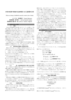
![名前:解答例 問題6 (1) 純アルミニウムにおいては、 eV /atom]、ASV /R](http://s3.paperzz.com/store/data/005656799_1-6de218d9e340e146495f2f9cbf2e9e02-250x500.png)